Numerical Analysis of Effects of Arms with Different Cross-Sections on Straight-Bladed Vertical Axis Wind Turbine


1
Faculty of Engineering, Tottori University, 4-101 Koyama-Minami, Tottori 680-8552, Japan
2
Graduate School of Engineering, Tottori University, 4-101 Koyama-Minami, Tottori 680-8552, Japan
3
Research Institute for Applied Mechanics, Kyushu University, 6-1 Kasugakoen, Kasuga, Fukuoka 816-8580, Japan
4
Graduate School of Engineering, Osaka University, Yamada-Oka, Suita, Osaka 565-0871, Japan
5
Faculty of Science and Engineering, Saga University, Honjo, Saga 840-8502, Japan
*
Author to whom correspondence should be addressed.
Energies 2019, 12(11), 2106; https://doi.org/10.3390/en12112106
Submission received: 31 March 2019
/
Revised: 21 May 2019
/
Accepted: 23 May 2019
/
Published: 1 June 2019
(This article belongs to the Special Issue Design, Fabrication and Performance of Wind Turbines 2019)
Abstract
:Most vertical axis wind turbines (VAWTs) need arms connecting the blades with the rotational axis. The arms increase the power loss of VAWTs; however, the distribution between the pressure and friction influences and their degrees of influence have not yet been investigated in detail in past research. We applied computational fluid dynamics (CFD) targeting a small-sized straight-bladed VAWT to elucidate the effects of arms on turbine performance. In the analysis, three kinds of arms with different cross-sections (NACA 0018 airfoil, 18% rectangular, circular) with the same height were added to an armless rotor. The tangential forces and resistance torques caused by the added arms were recalculated by dividing the pressure and friction influences based on the surface pressure and friction distributions obtained by the CFD on an arm or a blade. The pressure-based tangential force of an arm, regardless of the cross-section, had a tendency to increase near the connection part between the arm and a blade. Though the value was small, the friction on the rectangular arm generated a driving force, whereas the friction on the other arms generated resistance forces. The pressure-based tangential force of a blade increased for a wide region around the connection part. The friction-based tangential force of a blade dropped around the connection part of every arm-equipped rotor. The arm resistance torque added to a VAWT by the existence of arms was larger than the added blade resistance torque in the cases of rectangular and circular arm rotors. Conversely, in the case of the airfoil arm rotor, the resistance torque added to blades became larger than that of arms.
1. Introduction
Lift-driven vertical axis wind turbines (VAWTs) represented by Darrieus turbine do not depend on wind direction from the rotor performance point of view and are highly efficient compared to horizontal axis wind turbines (HAWTs) when operating at high tip speed rotation. As large-scale offshore wind power systems are expected to take advantage of the characteristics of VAWT [1,2] or wind farm with many small-scale VAWTs [3], many studies on VAWT have been conducted [4]. Hara et al. [5] have been developing the Butterfly Wind Turbine (BWT), which is a kind of VAWT aiming to be a low-cost renewable energy source for drylands or other various places. Many studies and applications of water or tidal current vertical axis turbines have been reported [6,7,8]. The performance of the lift-driven vertical axis turbines depend largely on the cross-section of the main blades and the structure of whole rotor, which is the aspect ratio and solidity of the rotor; therefore, most studies focused on the main blade performance or rotor structure. Especially in numerical studies of vertical axis turbines, two-dimensional (2D) simulations are often conducted from the aspect of computational cost. Even in three-dimensional (3D) simulation, the calculation usually considers only the main blades [6,9]. For example, Orlandi et al. [10] analyzed the performance of an H-type VAWT in an inclined condition of the rotational axis from the vertical using 3D-computational fluid dynamics (CFD). They showed that the power gain in skewed flows was obtained mainly during the downwind phase of revolutions; however, the rotor model of the CFD had no arms. Alaimo et al. [11] investigated the effects of computational conditions such as the mesh size on the CFD of a straight-type VAWT and compared the 2D and 3D computations. The performances of a straight-type VAWT and a helical-type VAWT were compared and, as a result, the helical type performed better than the straight type at a low tip speed ratio (TSR). Only the blades were considered in those rotor models. Li et al. [12] conducted wind tunnel experiments with a two-bladed VAWT and compared the results with the 3D-CFD. The experimental turbine had two-stage arms; the CFD model, which showed better performance than the power obtained experimentally using six-component balance, had no arms. However, the distribution along the blade span of the power coefficient obtained from pressure measurements illustrated the 3D effects caused by blade tips and arm existence. Subramanian et al. [13] investigated the effects of the airfoil and solidity on the performance of VAWT and showed that thick airfoils perform better at low TSR than thin airfoils, and that two-bladed turbine generated more power than three- or four-bladed turbines. Although the turbine models included a rotational axis, arms were not considered in the CFD computations.
Lift-driven VAWTs, however, need arms or struts, which connect the main blades to the rotational center axis, unlike HAWTs, though a vertical axis turbine equipped with the endplates as large as the rotor diameter, like a cross-flow turbine [14], and the BWT [5,15] may not need the arms. The arms act as fluid resistance and, more or less, cause a loss on the vertical axis turbine. Islam et al. [16], in the analysis of design parameters of a fixed-pitch straight-bladed VAWT, described the type classification, cross-section shape, and importance of the supporting struts, i.e., arms. Li and Calisal [17] investigated the effects of the arms of vertical axis tidal current turbines using experiments and numerical simulations. As shown by these previous studies, an airfoil shape with an ideal smaller drag coefficient should be selected for the arm cross-section to minimize the loss caused by the arms. For example, Ramkissoon et al. [18] searched for an airfoil shape that could be applied to the horizontal strut-arms of VAWTs and could have the lowest drag coefficient among four base airfoils using the XFOIL program [19] with an optimization method.
However, as Islam et al. [16] described, the arms need enough strength to support the blades and should be inexpensive; therefore, there is a tradeoff between the aerodynamic performance, i.e., drag coefficient, and the structural strength of arms. Accordingly, the arm cross-section does not necessarily have an airfoil shape in the cases of some practical VAWTs or in the cases of VAWT models for the studies aimed at practical application. Qin et al. [20], for instance, compared the 3D-CFD results on three-bladed H-type VAWT (rotor diameter: 2.5 m) with circular arms (arm diameter: 0.064 m) with the 2D-CFD results without arms, and showed that the average torque of 3D-CFD was 40% less than that of 2D-CFD. Note that the loss included the blade tip loss. Shires [2], in the aerodynamic model based on blade element momentum (BEM) theory, targeted a unique offshore V-shaped VAWT with a multi-blade structure with the struts in an elliptical profile and considered the profile drag coefficient [21] arising from the arm-surface pressure and the secondary drag coefficient [22] related to the arm-blade junction. Those drag coefficients were obtained from wind tunnel experiments in which the models were fixed under a constant wind speed.
In the operation of a VAWT, whose rotational axis is perpendicular to the main flow, the direction, or angle of attack, of the relative flow to a blade or an arm changes during rotation; therefore, because the local tangential forces change too, the averaged tangential force coefficients should be different from the drag coefficient obtained experimentally under stable flow. The secondary drag coefficient proposed by Roach and Turner [22] is attributed to a strut-blade connection but includes no influence on blades. To the best of the authors' knowledge, the degree of influence on the aerodynamic degradation (i.e., increase in tangential force or decrease in lift) of blades by the existence of the arms of a VAWT has not yet been sufficiently investigated. The drag arises from both pressure and friction on the surface of an object body. Although there are many reports about various objects and conditions regarding the pressure and friction drags [23], the degrees and the distribution ratio of the two drags have not yet been examined in the case of VAWT.
In this study, computational fluid dynamics (CFD) analyses targeting a small-sized two-blade VAWT were conducted assuming cases with horizontal arms (struts) of three different cross-sections and without arms. The distributions of pressure and friction, or shear stress, on the surfaces of the arms and blades were investigated, then their values were integrated with in-house software to obtain the pressure-based and friction-based tangential forces of each arm and blade. Subsequently, the resistance torques generated by the existence of the arms were calculated and the influences of the arm existence and the arm cross-section shape on the VAWT performance were discussed. The distribution ratios of the added resistance torque of each rotor equipped with the respective arms between the arms and the blades and between the pressure and the friction effects are identified here.
2. Methods
The wind turbine rotor targeted for calculation is described in Section 2.1. In Section 2.2., after the description of the calculation conditions of CFD analysis, the flow fields around each wind turbine rotor are assumed and the power coefficients are shown. Then, a simple theoretical prediction of the arm resistance torque based on the aerodynamic data and the influence of the arms on each rotor determined by the CFD are compared in Section 2.3. In the last subsection, the method used to analyze the pressure-based and friction-based tangential force coefficients of the arms or blades is explained.
2.1. Wind Turbine Rotor Targeted for Calculation
The base of wind turbine rotors targeted for the present study was the same H-type Darrieus turbine as the two-blade experimental wind turbine (DU-H2-5075) [24,25] (Figure 1). The rotor size parameters are shown in Table 1. The blade airfoil is NACA 0018.
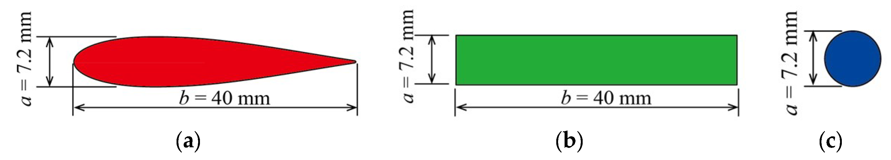
The experimental rotor had two-stage horizontal arms; however, the details of the shape and size were unknown. In the calculation, we targeted the base wind turbine rotor without arms and three rotors with two-stage arms; each arm cross-section of the three rotors is (1) an airfoil shape, (2) a rectangular shape, and (3) a circular shape, as shown in Figure 2, and is uniform along the span. The cross-section of the airfoil arm is the same NACA 0018 as the blade, but the chord length b is 40 mm and the maximum thickness a is 7.2 mm. Accordingly, the cross-section of the rectangular arm is a × b = 7.2 mm × 40 mm and the diameter of the circular arm is a = 7.2 mm. Each arm is installed in 25% or 75% of the blade span. The 40% position of the blade chord from the leading edge coincides with the center of each arm cross-section at the far arm edge from the rotor center, where the blade chord line is normal to the center axis of each arm.
As with the experimental conditions [26], the upstream wind speed U∞ was assumed to be 7 m/s in this study. The rotational speed of the wind turbine was set to 535 rpm (λ = 3), which is almost the same as the optimal condition (λ = 2.9) of the experimental rotor in the case of no inclination of the rotational axis. The rotational conditions are tabulated in Table 2.
The 2D drag coefficient CD of each arm against a uniform flow is defined by the frontal area of the arm per unit length, that is, by the arm height a [27]. If the representative flow speed is defined by the averaged relative flow speed at the maximum radius position, that is, the blade tip speed Rω, the CD of the airfoil arm is 0.11 [28] (Reb = 5.6 × 10⁴), the CD of the rectangular arm is 0.97 [27] (Reb = 5.6 × 10⁴), and the CD of the circular arm is 1.2 [27] (Rea = 1.0 × 10⁴). Here, Reb is the Reynolds number based on the length of the cross section parallel to the main flow, defined by Reb = bRω/ν. In the case of a circular arm, because the length parallel to the main flow is the diameter a, the Reynolds number is expressed by Rea. The length of each arm L is assumed to be 355 mm. The hub and the rotational axis of each turbine rotor are not considered in the CFD analysis described below.
2.2. CFD Analysis
2.2.1. Computational Conditions and Computational Mesh
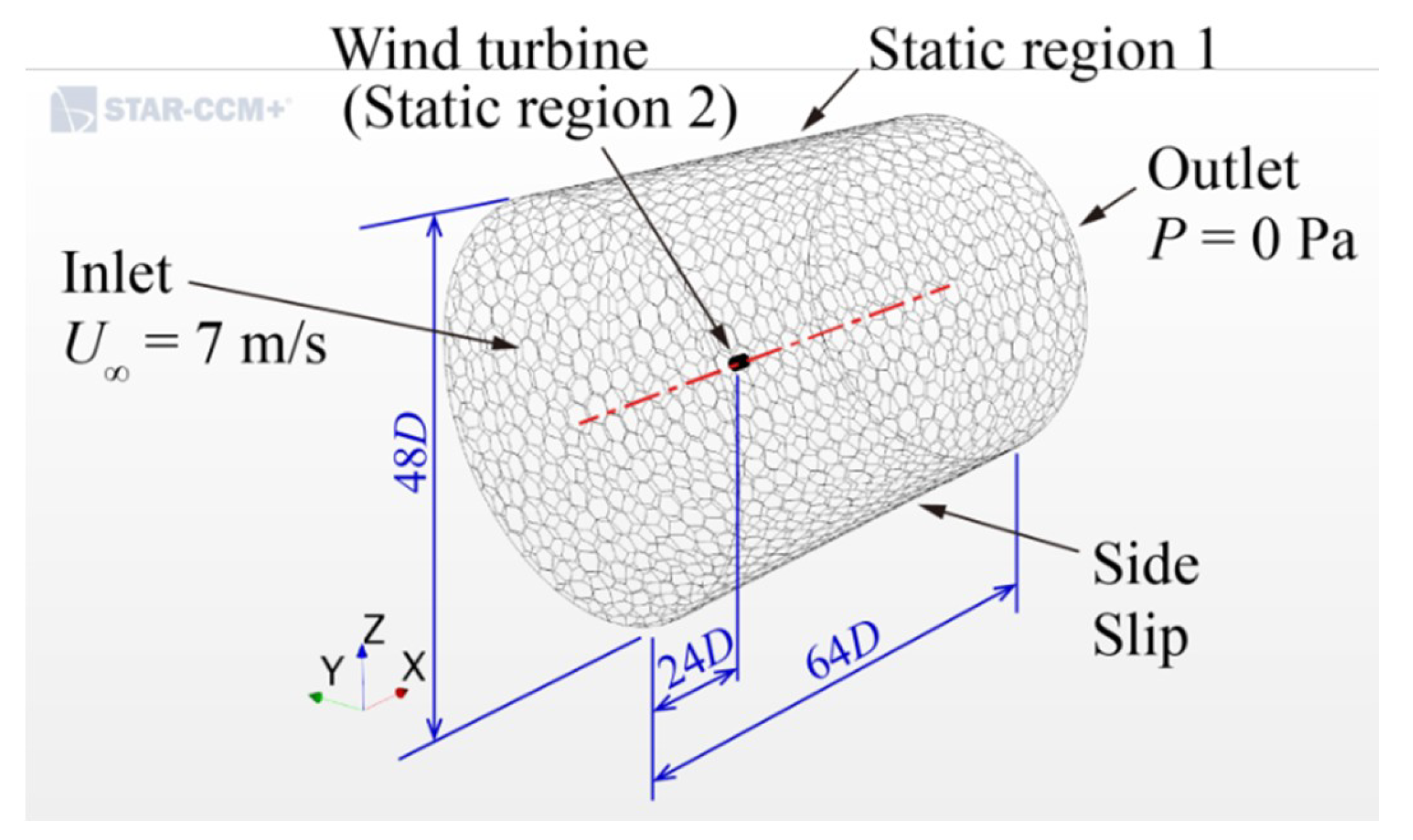
The solver used for CFD analysis in this study was the STAR-CCM+, which is a CFD- focused multiphysics simulation software of Siemens PLM Software. The Reynolds averaged Navier-Stokes (RANS) equations and the equation of continuity are solved simultaneously under the conditions of 3D incompressible fluid in unsteady state with the SST (Shear Stress Transport) k–ω turbulence model [29]. The whole computational domain (static region 1) is the inside of a cylindrical column of the diameter of 48D with the length of 64D, as shown in Figure 3. The center of the wind turbine rotor is located 24D downstream of the inlet boundary. A constant flow speed of U∞ = 7 m/s is provided at the inlet boundary, a constant gauge pressure of P = 0 Pa is given at the outlet boundary, and a slip condition is imposed on the side surface of the static region 1.
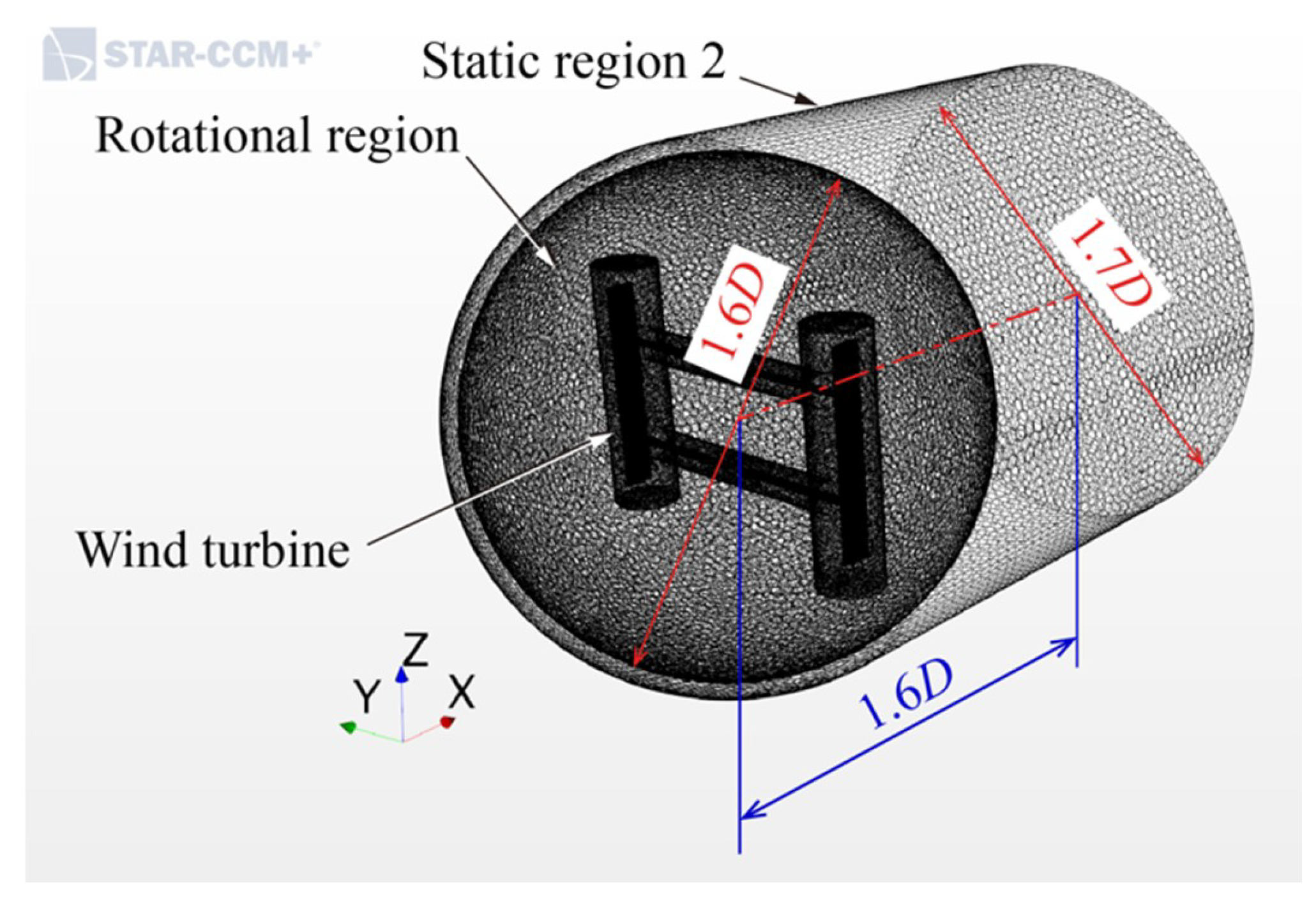
Figure 4 shows the regions around the wind turbine model, which was built in a spherical volume (rotational region) with a diameter of 1.6D. The rotational region is surrounded by a static region (static region 2), which consists of a hemisphere with the radius of 0.85D and a cylindrical column with the length of 1.6D to adjust the mesh size.
The unstructured polyhedral mesh was adopted in most of the computational domain except for regions close to the surfaces of blades and arms, where prism layer mesh was generated in 15 layers. The minimum mesh size near the blade surface was about 1.15 × 10⁻⁶ m, which corresponds to y+ of about 0.35. To check the grid independence, preliminary calculations on the armless rotor were performed under the condition of λ = 3 in the cases with total cell numbers of 5.05, 6.62, 7.75, 9.29, and 10.55 million. The torque variations in a blade in those grid cases are compared in Figure A1. All the results coincided within 1% of the mean value Cp = 0.24 of the power coefficients calculated for the 5 mesh cases. So, the mesh with 6.62 million cells in total was adopted for the armless rotor. By adopting the equivalent mesh, the total mesh-cell number was 11.12 million in the airfoil arm rotor, 11.50 million in the rectangular arm rotor, and 8.87 million in the circular arm rotor. In all the cases, the summed mesh-cell number in the static regions 1 and 2 was 0.58 million. The mesh state generated in the vicinity of the rotational region and around a blade is illustrated on an equatorial plane in Figure 5.
A time step was fixed at Δt = 1.558 × 10⁻⁴ s. The rotor revolved 0.5 degrees per time step. Each calculation was completed until 7 revolutions to obtain the convergence.
2.2.2. Results of CFD Analysis Regarding the Rotor Performance
The state of vortex shedding from each rotor at the end of 7 revolutions (time level: 5040) is depicted in Figure 6 with the Q-criterion (second invariant of velocity gradient) isosurfaces (Q = 200 s−2) [30], on which the vorticity magnitude is expressed using color contour (see the Supplementary Materials including the animations of vortex shedding). Figure 6d depicts the case of the armless rotor, in which strong arc-shaped tip vortices are shed from both ends of each blade when a blade passes through the upwind half of the rotor. Blade 2 is in the position of azimuth Ψ = 180° in Figure 6d; the almost uniform vertical vortex built by the dynamic stall [31] is shed from the trailing edge around the equator of Blade 2. In addition to the above-mentioned vortex, vortices are shed from the arms in the rotors equipped with arms in Figure 6a–c. Especially in the circular arm rotor shown in Figure 6c, the vortices that are related to the Karman vortex streets are shed in the wake of the arms. The vortex shedding from the trailing edge of each airfoil arm in Figure 6a, which is a small amount and hardly observable, should be attributed to the outflow of the boundary layer. As the vortex shedding from the blades are complicated in the rotors equipped with arms, the existence of the arms has a considerable influence on the flow field around the blades. As shown in Figure 6a,b, a loop-like vortex is shed from each of the junction parts of the airfoil and rectangular arm rotors. Judging from the strength of the vortex, it is not the horse-shoe vortex formed around the juncture illustrated by Roach and Turner [22]. The loop-like vortex might be derived from bound vortices of the blade.
The power coefficients Cp are compared in Figure 7. The circles in black are experimental results [26]. The calculation results of CFD analysis of the armless rotor and the airfoil arm rotor, which had been obtained for the rotational conditions before and with λ = 3, are also shown in Figure 7. The power coefficients of the armless rotor are larger than those of the experiments and reach the maximum at λ = 3. Coincidentally, the power coefficients of the airfoil arm rotor agree well with those of the experiments. The power coefficients of the circular and rectangular arm rotors at λ = 3 are negative (−0.022 and −0.138) and the two rotors do not operate as wind turbines. Not shown in Figure 7, in the case of the rectangular arm rotor with the arms of half thickness (a = 3.6 mm), the power coefficient takes a slightly positive value (Cp = 0.013) at λ = 3.
2.3. Comparison of Total Arm Influence between CFD and a Simple Theory
It is possible to estimate the resistance torque caused by the horizontal arms (or struts) of a VAWT, provided that the drag coefficient of the arm is given. Using the drag coefficient CD defined on the basis of the frontal area, the drag force FD acting on a 2D body with unit span and the height a normal to the flow is defined by Equation (1):
where Ur is the relative flow speed and ρ is the fluid density.
As the origin of azimuth Ψ is set in the perpendicular direction to the main flow in this study (Figure 9a), the relative flow speed Ur at a local radius r is expressed as:
where ω is the rotor-rotation angular velocity. In Equation (2), the induced flow velocity within the rotor is not considered.
Assuming that the number of blades is B and the number per blade of arms (struts) is S, the average resistance torque QTA generated by all the arms of a straight-bladed VAWT is calculated by:
where r0 is the distance between the rotational center axis and the inner end of an arm. The distance is assumed to be r0 = 20 mm in the present study.
Substituting Equations (1) and (2) into (3), the theoretical total arm resistance torque QTA is calculated as:
where, in the derivation process, the relation ω = λU∞ /R is used.
Finally, changing Equation (4) into a non-dimensional form on the basis of the dynamic pressure of upstream speed U∞ and the rotor-swept area A = 2HD = 4HR, the total arm resistance torque coefficient is obtained:
In Figure 8, the total influences of all the arms, which were obtained from the results of CFD analysis by subtracting the armless rotor torque from each arm-equipped rotor torque, are compared with the values estimated using Equation (5). The drag coefficient CD of each arm was assumed to take the value evaluated at the maximum local radius, i.e., the rotor radius R (see the caption of Figure 2). The theoretical values of CQTA of these three kinds of arms with a height of a = 7.2 mm are proportional to the CD value. As the results of CFD analysis are liable to increase with the increasing drag coefficient, they are not linear to the CD value, unlike the theory. The proximity between the CFD and the theoretical values of the circular arm rotor is a coincidence.
The CD used in theory is constant and is estimated at the far end of the arm as mentioned above; conversely, the tangential force coefficient calculated in the CFD might vary along the arm span, where the Reynolds number should decrease with the decreasing relative flow speed. A large difference exists between the CFD and the theoretical values in both the airfoil arm rotor and the rectangular arm rotor, which is especially large for the rectangular arm rotor. The difference is supposedly caused from the losses in the connection parts and the blades because the length b parallel to the relative velocity in the airfoil and rectangular arms is larger than that in the circular arm. We analyzed the individual influence of the pressure and friction on each surface of the arms and blades to prove the validity of the supposition.
2.4. Analytic Method of the Pressure-Based and Friction-Based Tangential Forces on Arms and Blades
The forces acting on an arm or a blade are calculated from the respective distributions of surface pressure (gauge pressure Δp) and surface friction (tangential component of wall shear stress τW) obtained from the CFD analysis. Figure 9a provides the definition of azimuth Ψ. The coordinates x1, y1 fixed on a blade are also shown in Figure 9a to define the forces (Fqx1, Fqy1) acting on the blade that are ascribed to the surface pressure (q = p) or the surface friction (q = f). Fqx1 is the tangential force of the blade, and Fqy1 is the normal force and is not considered in this study.
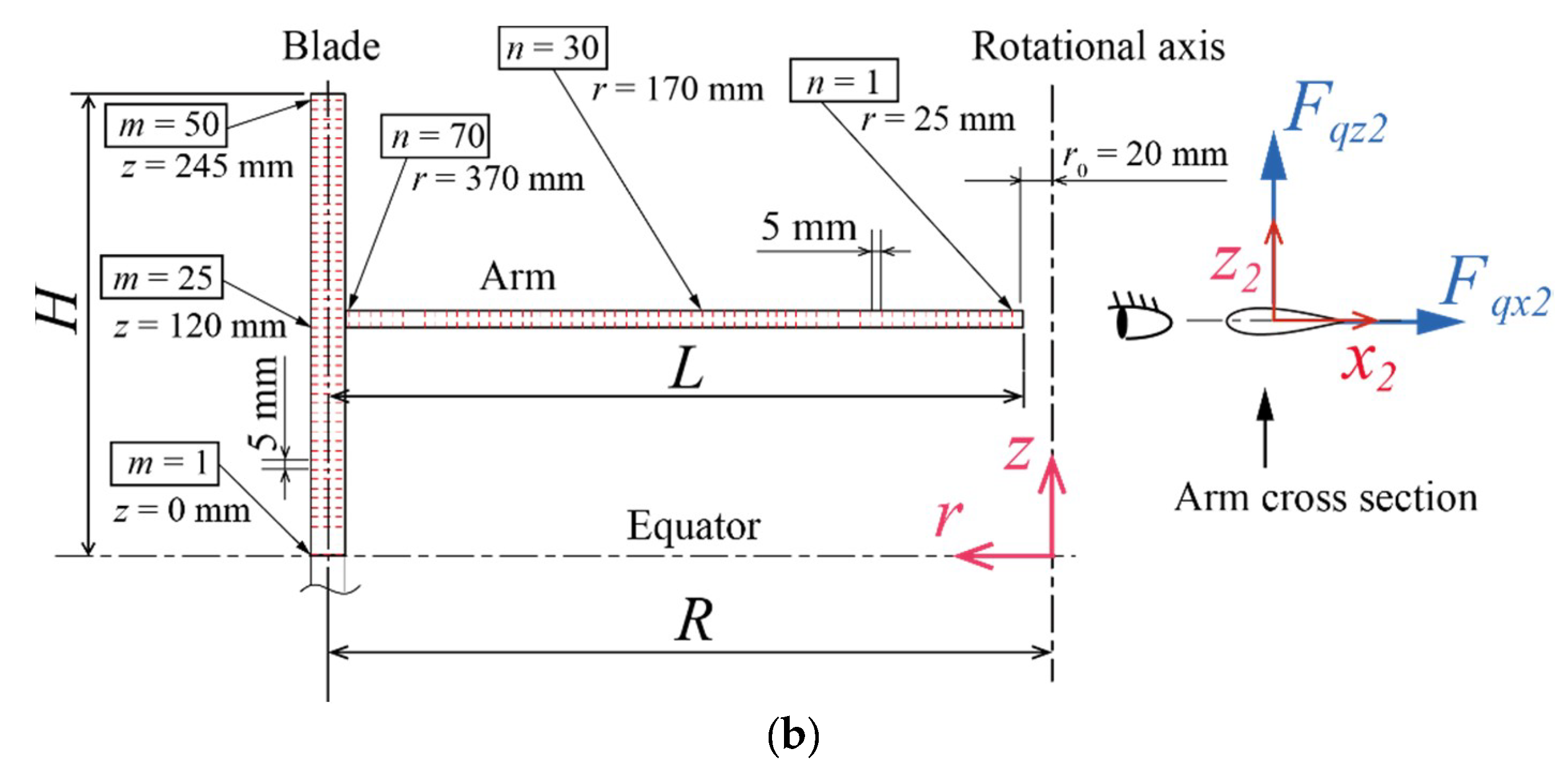
Figure 9b depicts the positions where the distributions of the surface pressure and the surface friction were extracted. For a blade, 50 cross-sections at intervals of 5 mm were selected from the upper half span (length H) with the equatorial plane (z = 0 mm) as the starting point. For the arm, 70 cross-sections at intervals of 5 mm were chosen between r0 and R in the radial direction. The coordinates x2, z2 fixed on an arm are depicted in Figure 9b to define the forces (Fqx2, Fqz2) acting on the arm that are ascribed to the surface pressure or friction. Fqx2 is the tangential force component parallel to the drag of the arm; Fqz2, which corresponds to the lift, is not considered in this study.
In an arbitrary cross section selected for extraction, the pressure-based and friction-based forces per unit span length acting in the x direction on a blade or an arm are calculated using Equations (6) and (7), respectively:
where the surface pressure Δp and the surface friction τW can be obtained from the CFD analysis, parameter s is the coordinates along the cross section boundary of an arbitrary two-dimensional object, the angle θ(s) is defined as the angle between the surface tangential and the x coordinate axis (Figure 10), the subscript j distinguishes the blade (j = 1) and the arm (j = 2), and the superscript l indicates the positions of extraction cross section (m = 1–50 or n = 1–70). The forces vary with the change in azimuth. Therefore, the forces defined in Equations (6) and (7) are calculated at intervals of 10 degrees in the azimuth in the seventh revolution of each rotor (Ψ = 10°, 20°, …, 360°). Note that y is replaced with z in Equation (6) and Figure 10 when the forces (Fnpx2(Ψ) and Fnfx2(Ψ)) acting on the arms are calculated.
In the present study, the non-dimensional force coefficient in the xj direction is defined as follows:
where the representative flow speed in the denominator is the maximum average tip speed Rω corresponding to the average relative flow speed and a is the arm height. Therefore, the non-dimensional force coefficient is equivalent to the drag coefficient CD of the arms (cf. Equation (1)). However, because the thickness of the blades is 2a, the value by Equation (8) for the blades (j = 1) corresponds to twice as large a value as the tangential force coefficient of the blades.
The non-dimensional force coefficients are averaged during one rotor revolution at each extraction cross section (l = m or n) by Equation (9):
An example showing the azimuth dependency of the non-dimensional force coefficient defined by Equation (8) and the average calculated by Equation (9) is provided in Figure A2.
The rotationally averaged force coefficients are averaged using Equation (10) in terms of a blade span; similarly, the average in terms of an arm span is calculated using Equation (11):
The data from Equations (6) to (9) were processed using in-house software with the results of the CFD analysis as the input data in this study.
3. Results
According to the method described in the Section 2.4., the distributions of the surface pressure and the average tangential force coefficient based on the pressure were analyzed and are shown in Section 3.1, and those of the surface friction and the average tangential force coefficient based on the friction are shown in Section 3.2. In Section 3.3., by distinguishing or integrating the influences of pressure and friction, the resistance torques generated at the arms and blades, by the existence of the arms are considered.
3.1. Tangential Force Based on Surface Pressure
3.1.1. Distributions of Pressure
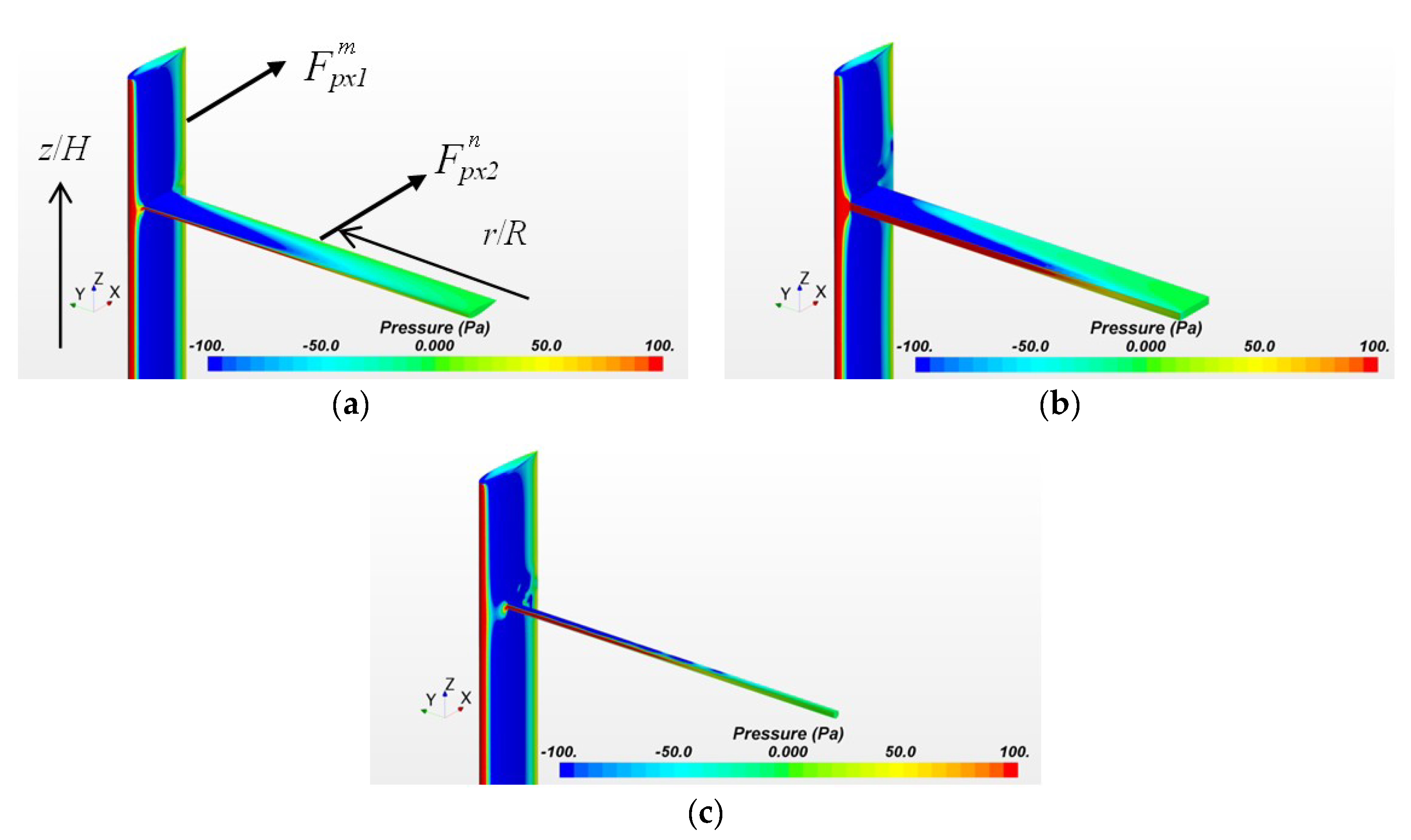
The distributions of surface pressure on each arm and blade of the respective rotors with three kinds of arm cross-sections are illustrated in Figure 11 (see the Supplementary Materials including the animations of the pressure distributions). Figure 11 shows the conditions at the end of seven revolutions (Ψ = 0°); the reddish colors indicate positive pressure and the bluish colors, negative pressure. The surface pressure varies considerably along each arm span in all the arm-equipped rotors. Differences among the rotors in the pressure distribution on the blade surface are observed around the connections between the arm and the blade.
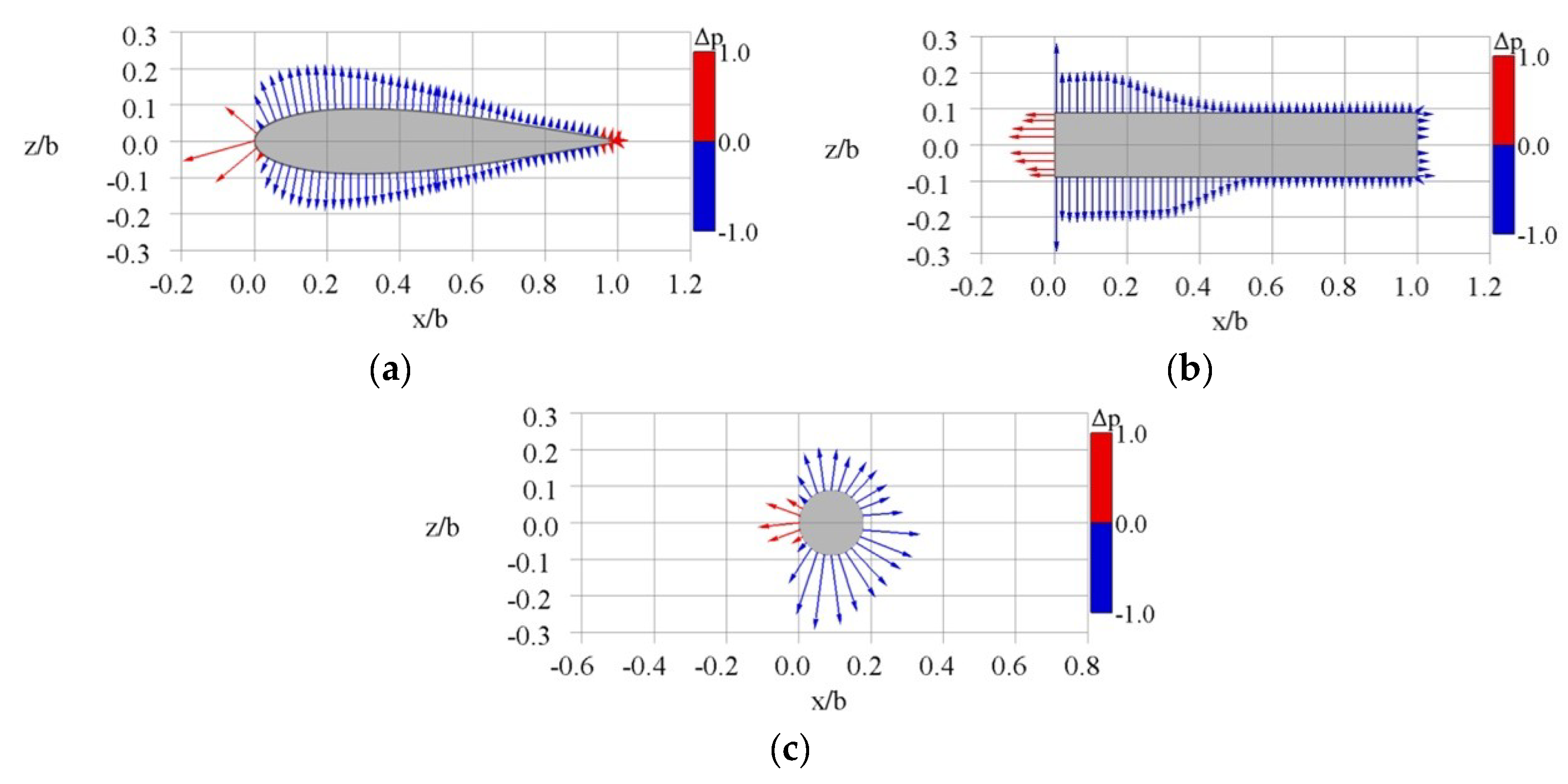
Figure 12 illustrates the surface pressure distributions around the cross sections of n = 30 (r/R = 0.453) of the arms under the same condition (Ψ = 0°) as in Figure 11. In each distribution shown in Figure 12, red vectors express positive pressure and blue vectors express negative pressure. All the vectors are depicted oriented outward and normal to the surface, and the length of the vectors is proportional to the absolute of the gauge pressure Δp. All the coordinates in Figure 12a–c are non-dimensional on the basis of the flow direction length (b = 40 mm) of both airfoil and rectangular arms. The pressure distributions are somewhat asymmetric in the vertical direction because the upper arms are depicted in Figure 12 and the flow passing across the upper arms is oriented upward due to the expanse of the flow.
Figure 13 illustrates the surface pressure distributions around the cross-sections of m = 25 (z/H = 0.480) of the blades under the same condition (Ψ = 0°) as in Figure 11. These blade cross-sections are located just below the connection parts; the lower surface of each blade in Figure 13 corresponds to the inside of the rotors where the arms exist. Compared with the case of the armless rotor shown in Figure 13d, the surface pressure of the blade on the inner side is affected greatly by the arms, as shown in Figure 13a–c.
3.1.2. Distributions of Average Pressure-Based Tangential Force
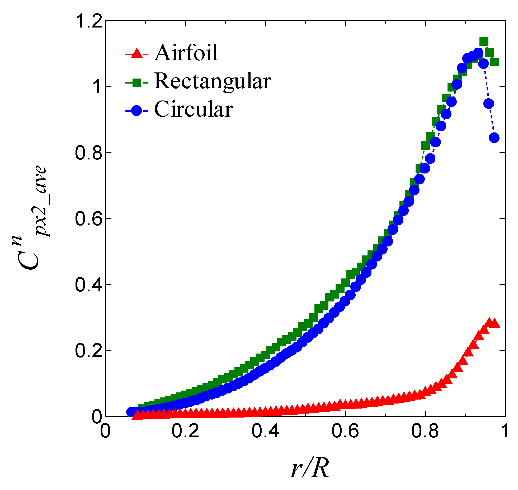
The distributions along each arm span of the non-dimensional pressure-based force coefficients (Cnpx2_ave) averaged rotationally using Equation (9) are shown in Figure 14. The force coefficients, i.e., the drag coefficients, have a tendency to increase when approaching the connection part (r/R = 1) regardless of the arm cross-section shape, which could be accounted for by the increasing local relative flow speed.
The pressure-based tangential force coefficients averaged along the arm span direction by Equation (11) are shown in Table 3. The average pressure-based tangential force coefficient of the rectangular arm is 0.415, which is the largest. The value of the airfoil arm is 0.050, about 10 times smaller than that of the rectangular arm.
Figure 15 shows the distributions along the half-blade span of the non-dimensional pressure-based force coefficients (Cmpx1_ave) averaged rotationally by Equation (9); the positive direction of the force is the x1 direction defined in Figure 9a. The force coefficients of the armless rotor are approximately constant in the range of 0 < z/H < 0.7 and take negative values. This means that a local blade element on average generates a driving force in the –x1 direction. The driving force decreases toward the blade tip (z/H = 1), showing the effects of the blade tip loss. In all the cases of arm-equipped rotors, the driving force decreases around the connection (z/H = 0.5); in other words, the pressure-based tangential force increases there. Especially for the rectangular arm rotor, the pressure-based tangential force increases at the wider region of the blade. An extensive increase in the tangential force is observed in the airfoil arm rotor, which is not as much of an increase as in the rectangular arm rotor. The influence of the circular arm on the blade is relatively small.
The pressure-based force coefficients () obtained by averaging the values of Cmpx1_ave along the half-blade span direction by Equation (10) are shown in Table 4. The bottom row of Table 4 shows the pressure-based tangential force coefficients () corresponding to the increase in the resistance of each blade, which were obtained from the difference between each averaged force coefficient and that of the armless rotor. The pressure-based tangential force added to the blades by the existence of the rectangular arms is 1.82 times as large as that of the airfoil arms; the case of the circular arms is 0.67 times as large as the case of the airfoil arms.
3.2. Tangential Force Based on Surface Friction
3.2.1. Distributions in Friction Force
The distributions in the x-direction wall shear stress on each arm and blade in the respective rotors with three kinds of arm cross-sections are illustrated in Figure 16 (see the Supplementary Materials including the animations of the wall shear stress distributions). Figure 16 shows the conditions at the end of seven revolutions (Ψ = 0°); the reddish colors indicate the surface friction pointing in the positive x-direction (x1 or x2 directions) and the bluish colors point in the opposite direction. A blue-colored region is widely observed near the front edge on the upper surface of the rectangular arm in Figure 16b, which is different in appearance from the other arms.
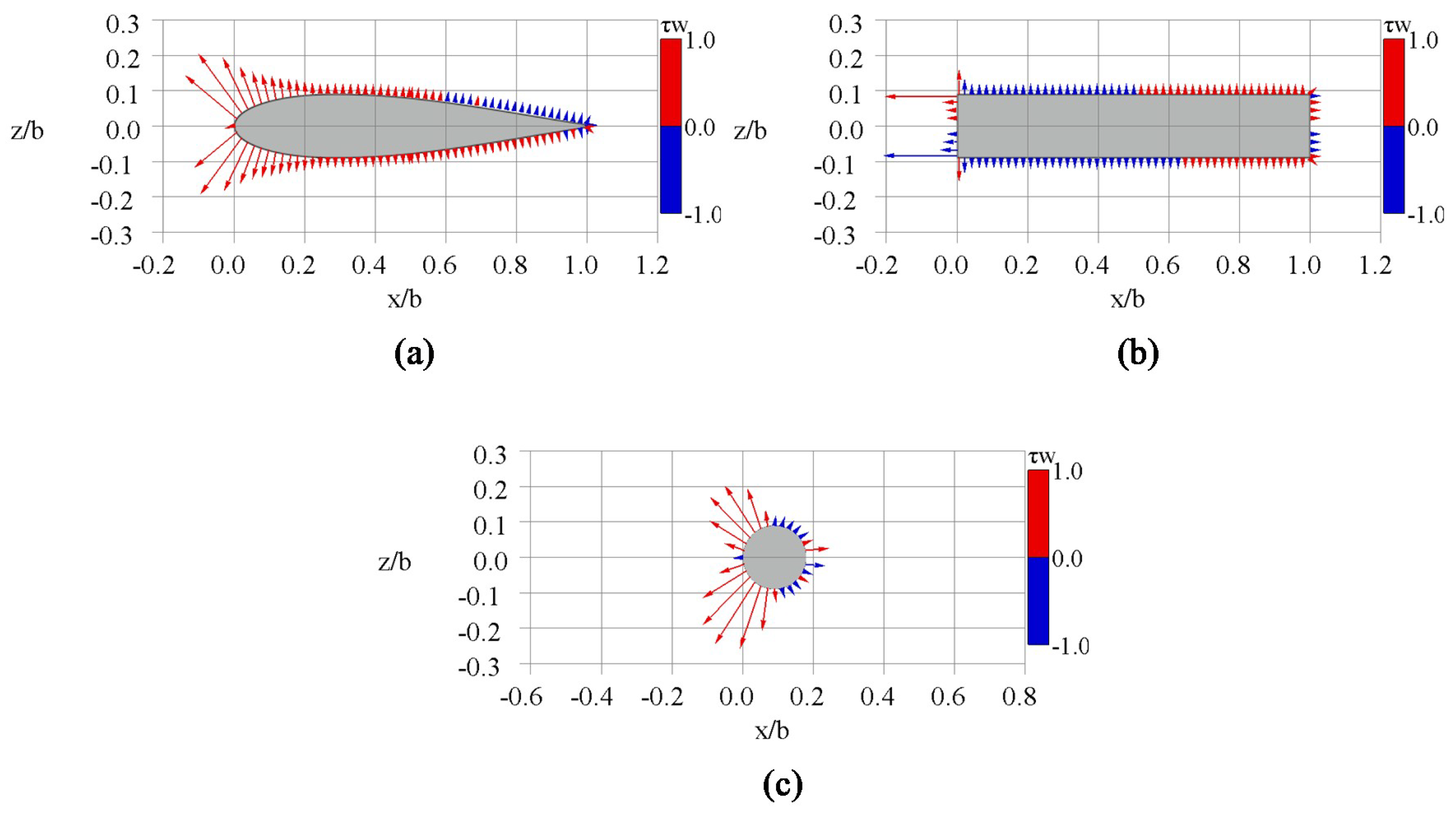
Figure 17 illustrates the distributions of the tangential component (τw) of the wall shear stress around the cross-sections of n = 30 (r/R = 0.453) of the arms under the same condition (Ψ = 0°) as in Figure 16. The red vector indicates the x component of wall shear stress is positive and the blue vector indicates the opposite state. On the left and right end surfaces of the rectangular arm in Figure 17b, however, the color of vector is red when the z component of wall shear stress is positive (upward), and is blue in the opposite state. All the vectors are depicted oriented outward and normal to the surface, and the length of the vectors is proportional to the absolute of the surface friction τw. At the front portion of the upper and lower surfaces of the rectangular arm, the x component of wall shear stress is negative; this shows that the separations occur from the front edges and the counter-flows occur on the surfaces near the frontal edges.
Figure 18 illustrates the distributions of the tangential component (τw) of the wall shear stress around the cross-sections of m = 25 (z/H = 0.480) of the blades under the same condition (Ψ = 0°) as in Figure 16. In the case of the armless rotor in Figure 18d, most of the wall shear stress has a positive x component acting as the friction in the direction from the leading edge to the trailing edge. On the blade cross-sections located just below the connection parts in Figure 18a–c, the negative x components of wall shear stress, i.e., counter-flows, occur in wide regions on the inner side; the existence of arms has a complicated influence on the flow directions near the blade surface.
3.2.2. Distributions of Average Friction-Based Tangential Force
The distributions along each arm span of the non-dimensional friction-based force coefficients, (Cnfx2_ave) averaged rotationally using Equation (9), are shown in Figure 19. The friction-based tangential force coefficients increases when approaching the connection part (r/R = 1) in the cases of the airfoil and circular arms. In contrast, the friction-based tangential force coefficient of the rectangular arm takes negative values in the region over r/R = 0.4 and the maximum value of the negative direction at r/R is about 0.75.
The friction-based tangential force coefficients averaged along the arm span direction using Equation (11) are shown in Table 5. The average friction-based tangential force coefficient of the airfoil arm is 0.024 and is the largest. The value of the rectangular arm is negative, which shows that the surface friction operates as the driving force on average.
Figure 20 depicts the distributions along the half-blade span of the non-dimensional friction-based force coefficients (Cmfx1_ave) averaged rotationally by Equation (9). The positive direction (x1 direction) of the force is oriented toward the wake of each blade. The force coefficients of the armless rotor are approximately constant in the range of 0 < z/H < 0.9 and increase close to the blade tip (z/H = 1), showing the effects of the blade tip loss. In all the cases of arm-equipped rotors, the friction-based tangential forces of the blades drop around the connection part (z/H = 0.5) due to the contact area of the arm and the blade. There is no definite difference among the arm-equipped rotors regarding the degrees of the drops and the fluctuations in the friction-based tangential force.
The friction-based force coefficients () obtained by averaging the values Cmfx1_ave along the half-blade span direction using Equation (10) are shown in Table 6. The bottom row of Table 6 shows the friction-based tangential force coefficients () corresponding to the increase in the resistance of each blade, which were obtained from the difference between each averaged force coefficient and that of the armless rotor, described in the middle row of the Table 6. The friction-based tangential force added to the blades by the existence of the rectangular arms is 1.77 times larger than that of the airfoil arms, whereas the case of the circular arms is 11% less than the case with airfoil arms.
3.3. Resistance Torque Induced by the Existence of Arms
In the previous sections, the distributions of the forces based on the pressure and friction acting on each portion of the arms and the blades were shown. Based on them, the resistance torques operating on the whole wind turbine rotor were calculated and are discussed in this section.
The non-dimensional resistance torque based on the pressure (q = p) or the friction (q = f) operating on all the arms of a rotor are obtained using Equation (12). Similarly, the non-dimensional resistance torque added to all the blades due to the existence of the arms is calculated using Equation (13):
where B is the number of blades and S is the number of arms (struts) per blade; in this study, B = 2 and S = 2. Unlike Equation (8), the resistance torque coefficients in Equations (12) and (13) are based on the upstream flow speed U∞, the rotor swept area A, and the rotor radius R.
Table 7 lists the results of the calculations of Equations (12) and (13) for the respective arm-equipped rotors. For the airfoil arm rotor, the resistance torque based on the pressure of the blades is large due to the existence of the arms. Although the value is small, the generation of driving torque based on the friction of the arms is conspicuous in the rectangular arm rotor. A large part of the additive resistance torque in the circular arm rotor is attributed to the pressure of the arms.
The coefficients of the additive resistance torques of a whole rotor based on pressure, friction, and both are determined using the following equations:
The results of calculation of Equations (14)–(16) regarding the respective rotors are tabulated in Table 8. The resistance torques caused by the friction due to the existence of the arms are one order less than those caused by the pressure. The total resistance torque of the rectangular arm rotor is largest, followed by that of the circular arm rotor. The values of CQ_total of the two rotors are 3.1 and 2.3 times as large as that of the airfoil arm rotor, respectively. The resistance torque coefficients CQ_total obtained according to the above-mentioned data processing agree well with the CFD results (CQTA) shown in Figure 8.
Table 9 shows the non-dimensional resistance torques added by the existence of arms to the arms or the blades, which were obtained using Equations (17) and (18):
The values in the parentheses in Table 9 are the ratios of each resistance torque coefficient to the total (CQ_total) in each arm-equipped rotor. The resistance torque of arms accounts for a large proportion of the cases of the rectangular and circular arm rotors. In the case of the airfoil arm rotor, the additive resistance torque of the blades are much larger than that of the arms.
4. Conclusions
For investigating the influence of arms, or struts, on VAWTs, 3D CFD analysis was conducted targeting the small, straight-bladed VAWT rotors with the NACA 0018 airfoil, 18% rectangular, and circular arms with the same height. Based on the CFD results, the tangential forces and resistance torques induced by the arms were decomposed to the effects of pressure and friction.
In terms of the distributions of pressure-based tangential forces, the pressure-based tangential force coefficients of an arm had the tendency to increase with decreasing distance to the connection part regardless of the arm cross-section shape. The pressure-based tangential force along the blade span increased around the connection part. The widespread increase in the tangential force on the blade was especially observed in the rectangular arm rotor, followed by the airfoil arm rotor.
Regarding the friction-based tangential force distributions, we found that the flow separations occurred near the front edges of the rectangular arm, and the surface friction by the separation bubbles generated the driving force. The decreases in the friction-based tangential force were observed on the blades around the junctions; however, the differences were not clear among the different arm rotors in terms of the degrees of the drop and the variations in additive friction-based tangential force.
From the results of the integration of the resistance torque, we found that the additive friction effects were very small compared to the pressure effects. The total resistance torque of pressure and friction was the largest in the case of the rectangular arm rotor followed by that of the circular arm rotor—3.1 and 2.3 times as large as the airfoil arm rotor. As one of the important findings, the resistance torque induced on the arms was larger than that induced on the blades in the rectangular and the circular arm rotors. Conversely, the resistance torque induced on the blades was much larger than that induced on the arms in the airfoil arm rotor.
This study targeted a small VAWT. When considering larger wind turbines, some differences, such as the decrease in the pressure-based tangential force or the increase in the friction-based tangential force, could be expected due to the Reynolds number. If the manufacturing cost and structural strength of the arms are not a problem, however, the airfoil remains ideal for the arm cross-section shape.
We showed that the airfoil arms have much more influence on the blades than the arms. Islam et al. [16] categorized the types of blade-supports in straight-bladed VAWTs as: cantilever, simple, and overhang types. The wind turbine targeted in the present study corresponds to the overhang type, in which the influence of the arms widely reached the blade portions on both the upper and lower sides of each connection part, as shown in Figure 15. To reduce the influence of the supporting arms on the blades as much as possible, the simple type with the arms installed into the blade tips might be the best choice because the influenced blade-portions of the simple type with two-stage arms are geometrically equivalent to those of the cantilever type with one-stage arms in addition to the possible cancellation of the blade tip loss. As the slant blade parts of the butterfly wind turbine [5], which is explained as “armless”, corresponds to the arms of the simple type, the loss caused by the connection between the main vertical blade and the slant blade is expected to be small. However, even in the case of the simple- or the butterfly-type wind turbine, more supporting arms or braces than three stages are needed to restrain the deformation of the blades if the rotor size is large. In that case, it is important to consider the influence of the arm cross-section shape on the blades, in addition to the structural strength and the drag coefficient of the arms.
Supplementary Materials
The following are available online at https://www.mdpi.com/1996-1073/12/11/2106/s1, Video s1: Animations of Q-criterion isosurface (Figure 6), Surface pressure (Figure 11), and x-direction wall shear stress (Figure 16).
Author Contributions
Conceptualization, Y.H; methodology, Y.H.; software, Y.H.; validation, N.H., S.Y., H.A., and T.S.; formal analysis, Y.H. and N.H.; investigation, N.H.; resources, Y.H.; data curation, Y.H.; writing—original draft preparation, Y.H.; writing—review and editing, S.Y., H.A., and T.S.; visualization, N.H.; supervision, Y.H.; project administration, Y.H.; funding acquisition, Y.H. and H.A.
Funding
This research was supported by the International Platform for Dryland Research and Education (IPDRE), Tottori University, the Collaborative Research Program of Research Institute for Applied Mechanics, Kyushu University, and the Grant-in-Aid for Scientific Research (16H04599) from the Japan Society for the Promotion of Science.
Conflicts of Interest
The authors declare no conflict of interest.
Nomenclature
| a | Arm maximum thickness |
| A | Rotor swept area |
| b | Arm chord length |
| B | Number of blades |
| c | Blade chord length |
| CD | Two-dimensional drag coefficient based on frontal area per unit length |
| Cp | Power coefficient |
| Force coefficient in xj direction at position l based on pressure (q = p) or friction (q = f) | |
| Rotationally averaged force coefficient in xj direction at position l based on pressure (q = p) or friction (q = f) | |
| Span-wise averaged force coefficient in xj direction based on pressure (q = p) or friction (q = f) | |
| CQTA | Theoretical total arm resistance torque coefficient |
| CQ_arm | Total arm resistance torque coefficient caused by the existence of arms |
| CQ_blade | Total blade resistance torque coefficient caused by the existence of arms |
| CQ_f | Rotor resistance torque coefficient caused by friction |
| CQ_p | Rotor resistance torque coefficient caused by pressure |
| CQ_q_arm | Whole arm resistance torque coefficient caused by pressure (q = p) or friction (q = f) of arms |
| CQ_q_blade | Whole blade resistance torque coefficient caused by pressure (q = p) or friction (q = f) of blades |
| CQ_total | Rotor resistance torque coefficient caused by both pressure and friction |
| D | Rotor diameter |
| FD | Drag force |
| Flqxj(Ψ) | Force in xj direction at position l in azimuth Ψ based on pressure (q = p) or friction (q = f) |
| Flqxj_ave | Rotationally averaged force in xj direction at position l based on pressure (q = p) or friction (q = f) |
| H | Blade half span length |
| j | Suffix for distinguishing blade (j = 1) and arm (j = 2) |
| l | Superscript for distinguishing position parameters m and n |
| L | Arm length |
| m | Index indicating the position of extraction cross section of a half blade |
| n | Index indicating the position of extraction cross section of an arm |
| P | Constant gauge pressure |
| q | Suffix for distinguishing pressure (q = p) and friction (q = f) |
| Q | Second invariant of velocity gradient (Q-criterion) |
| QTA | Total arm resistance torque |
| r | Radial coordinate |
| r0 | Distance between rotational center axis and the inner end of an arm |
| R | Rotor radius |
| Re | Rotor Reynolds number |
| Rea | Reynolds number based on body height a perpendicular to the main flow |
| Reb | Reynolds number based on body length b parallel to the main flow |
| Rec | Blade Reynolds number |
| s | Coordinate along the cross sectional boundary of an arbitrary two-dimensional object |
| S | Number of arms (struts) per blade |
| Ur | Relative flow speed |
| U∞ | Upstream wind speed |
| x, y, z | Absolute coordinate |
| x1, y1 | Relative coordinate fixed on a blade |
| x2, z2 | Relative coordinate fixed on an arm |
| y+ | Maximum first cell height shown by non-dimensional coordinate with wall variable |
| Δp | Surface pressure (gauge pressure) |
| Δt | Time step |
| θ(s) | Angle between surface tangential and x coordinate axis at position s |
| λ | Tip speed ratio |
| ν | Dynamic viscosity of air |
| ρ | Air density |
| τw | Wall shear stress |
| Ψ | Azimuth |
| ω | Rotor-rotation angular velocity |
Appendix A
Figure A1 shows the mesh dependency of the torque variation of a blade of the armless rotor under the condition of λ = 3. The ordinate of the graph in Figure A1 is the torque coefficient defined as CT (Ψ) = T(Ψ)/0.5ρU∞2AR, where T(Ψ) is a torque acting on a blade as a function of the azimuth. The data of T(Ψ) obtained during the sixth revolution were used in each of different five mesh cases. Figure A1 shows that the mesh dependency of the torque variation is very small when there are 5.05 million cells or more.
Figure A1.
Mesh dependency of the torque variation of a blade of the armless rotor (λ = 3).

Appendix B
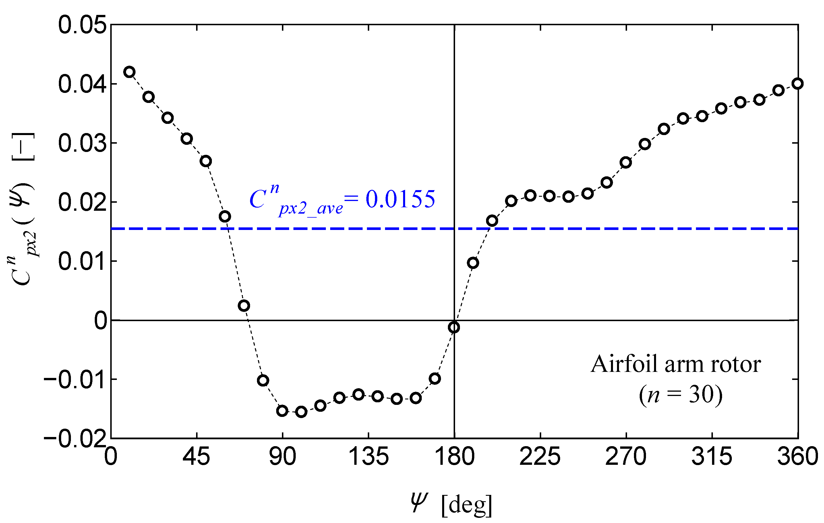
Figure A2 shows the azimuthal variation in the non-dimensional force coefficient defined by Equation (8) and the average calculated using Equation (9) at the cross-section of n = 30 of an arm of the airfoil arm rotor. In this example, the pressure-based tangential force in the x2 direction takes negative values when the arm moves in the range from 80° to 180° in the azimuth.
Figure A2.
An example showing the azimuth dependency of non-dimensional force coefficient.

References
- Borg, M.; Shires, A.; Collu, M. Offshore floating vertical axis wind turbines, dynamics modelling state of the art. part I: Aerodynamics. Renew. Sustain. Energy Rev. 2014, 39, 1214–1225. [Google Scholar] [CrossRef] [Green Version]
- Shires, A. Development and Evaluation of an Aerodynamic Model for a Novel Vertical Axis Wind Turbine Concept. Energies 2013, 6, 2501–2520. [Google Scholar] [CrossRef] [Green Version]
- Dabiri, J.O. Potential order-of-magnitude enhancement of wind farm power density via counter-rotating vertical-axis wind turbine arrays. J. Renew. Sustain. Energy 2011, 3, 043104. [Google Scholar] [CrossRef] [Green Version]
- Mendoza, V.; Bachant, P.; Ferreira, C.; Goude, A. Near-wake flow simulation of a vertical axis turbine using an actuator line model. Wind Energy 2019, 22, 171–188. [Google Scholar] [CrossRef]
- Hara, Y.; Tagawa, K.; Saito, S.; Shioya, K.; Ono, T.; Makino, K.; Toba, K.; Hirobayashi, T.; Tanaka, Y.; Takashima, K.; et al. Development of a Butterfly Wind Turbine with Mechanical Over-Speed Control System. Designs 2018, 2, 17. [Google Scholar] [CrossRef]
- Akimoto, H.; Iijima, K.; Hara, Y. Prediction of the flow around a floating axis marine current turbine. In Proceedings of the 2016 Techno-Ocean (Techno-Ocean), Kobe, Japan, 6–8 October 2016; pp. 272–275. [Google Scholar]
- Akimoto, H.; Tanaka, K.; Uzawa, K. A conceptual study of floating axis water current turbine for low-cost energy capturing from river, tide and ocean currents. Renew. Energy 2013, 57, 283–288. [Google Scholar] [CrossRef]
- Tsai, J.-S.; Chen, F. The Conceptual Design of a Tidal Power Plant in Taiwan. J. Mar. Sci. Eng. 2014, 2, 506–533. [Google Scholar] [CrossRef] [Green Version]
- Ghasemian, M.; Ashrafi, Z.N.; Sedaghat, A. A review on computational fluid dynamic simulation techniques for Darrieus vertical axis wind turbines. Energy Convers. Manag. 2017, 149, 87–100. [Google Scholar] [CrossRef]
- Orlandi, A.; Collu, M.; Zanforlin, S.; Shires, A. 3D URANS analysis of a vertical axis wind turbine in skewed flows. J. Wind Eng. Ind. Aerodyn. 2015, 147, 77–84. [Google Scholar] [CrossRef] [Green Version]
- Alaimo, A.; Esposito, A.; Messineo, A.; Orlando, C.; Tumino, D. 3D CFD Analysis of a Vertical Axis Wind Turbine. Energies 2015, 8, 3013–3033. [Google Scholar] [CrossRef] [Green Version]
- Li, Q.A.; Maeda, T.; Kamada, Y.; Murata, J.; Kawabata, T.; Shimizu, K.; Ogasawara, T.; Nakai, A.; Kasuya, T. Wind tunnel and numerical study of a straight-bladed vertical axis wind turbine in three-dimensional analysis (Part I: For predicting aerodynamic loads and performance). Energy 2016, 106, 443–452. [Google Scholar] [CrossRef]
- Subramanian, A.; Yogesh, S.A.; Sivanandan, H.; Giri, A.; Vasudevan, M.; Mugundhan, V.; Velamati, R.K. Effect of airfoil and solidity on performance of small scale vertical axis wind turbine using three dimensional CFD model. Energy 2017, 133, 179–190. [Google Scholar] [CrossRef]
- Sutherland, D.; Ordonez-Sanchez, S.; Belmont, M.R.; Moon, I.; Steynor, J.; Davey, T.; Bruce, T. Experimental optimisation of power for large arrays of cross-flow tidal turbines. Renew. Energy 2018, 116, 685–696. [Google Scholar] [CrossRef] [Green Version]
- Hara, Y.; Shiozaki, A.; Nishiono, H.; Saito, S.; Shioya, K.; Sumi, T.; Matsubara, Y.; Yasumoto, Y.; Takagaki, K.; Kogo, S. Experiment and numerical simulation of an aluminum circular-blade butterfly wind turbine. J. Fluid Sci. Technol. 2016, 11, JFST0010. [Google Scholar] [CrossRef]
- Islam, M.; Fartaj, A.; Carriveau, R. Analysis of the Design Parameters Related to a Fixed-Pitch Straight-Bladed Vertical Axis Wind Turbine. Wind Eng. 2008, 32, 491–507. [Google Scholar] [CrossRef]
- Li, Y.; Calisal, S.M. Three-dimensional effects and arm effects on modeling a vertical axis tidal current turbine. Renew. Energy 2010, 35, 2325–2334. [Google Scholar] [CrossRef]
- Ramkissoon, R.; Manohar, K.; Adeyanju, A. Horizontal Strut-Arm Optimization Effects on Drag Coefficient. Int. J. Innov. Res.Sci. Eng. Technol. 2015, 4, 11720–11726. [Google Scholar]
- Drela, M. XFOIL: An Analysis and Design System for Low Reynolds Number Airfoils. In Low Reynolds Number Aerodynamics; Mueller, T.J., Ed.; Springer: New York, NY, USA, 1989; Volume 54, pp. 1–12. [Google Scholar]
- Qin, N.; Howell, R.; Durrani, N.; Hamada, K.; Smith, T. Unsteady Flow Simulation and Dynamic Stall Behaviour of Vertical Axis Wind Turbine Blades. Wind Eng. 2011, 35, 511–527. [Google Scholar] [CrossRef]
- Hoerner, S.F. Fluid-Dynamic Drag; Hoerner Fluid Dynamics: Bricktown, NJ, USA, 1965; Volume 3–11. [Google Scholar]
- Roach, P.E.; Turner, J.T. Secondary loss generation by gas turbine support struts. Int. J. Heat Fluid Flow 1985, 6, 79–88. [Google Scholar] [CrossRef]
- Alfredsson, P.H.; Orlu, R. Large-Eddy BreakUp Devices-a 40 Years Perspective from a Stockholm Horizon. Flow Turb. Comb. 2018, 100, 877–888. [Google Scholar] [CrossRef]
- Mertens, S.; Van Kuik, G.; Van Bussel, G. Performance of an H-Darrieus in the skewed flow on a roof. J. Sol. Energy Eng. 2003, 125, 433–440. [Google Scholar] [CrossRef]
- Simão Ferreira, C.J.; Van Bussel, G.J.W.; Van Kuik, G.A.M. Wind Tunnel Hotwire Measurements, Flow Visualization and Thrust Measurement of a VAWT in Skew. J. Sol. Energy Eng. 2006, 128, 487–497. [Google Scholar] [CrossRef]
- Van Bussel, G.J.W.; Mertens, S.; Polinder, H.; Sidler, H.F.A. TURBY® concept and realisation of a small VAWT for the built environment. In Proceedings of the EAWE/EWEA Special Topic Conference: The Science of Making Torque from Wind, Delft, The Netherlands, 19–21 April 2004. [Google Scholar]
- White, F.M. Fluid Mechanics, 4th ed.; McGraw-Hill: New York, NY, USA, 1999; pp. 453–458. [Google Scholar]
- Sheldahl, R.E.; Klimas, P.C. Aerodynamic Characteristics of Seven Symmetrical Airfoil Sections through 180-Degree Angle of Attack for Use in Aerodynamic Analysis of Vertical Axis Wind Turbines; SAND-80-2114; Sandia National Labs: Albuquerque, NM, USA, 1981; pp. 43–44. [Google Scholar]
- Menter, F.R. Two-equation eddy-viscosity turbulence models for engineering applications. AIAA J. 1994, 32, 1598–1605. [Google Scholar] [CrossRef] [Green Version]
- Fu, W.-S.; Lai, Y.-C.; Li, C.-G. Estimation of turbulent natural convection in horizontal parallel plates by the Q criterion. Int. Commun. Heat Mass Transf. 2013, 45, 41–46. [Google Scholar] [CrossRef]
- Hara, Y.; Sumi, T.; Mizuguchi, S.; Akimoto, H.; Tanaka, K.; Kawamura, T.; Nakamura, T. 3D-CFD Analysis of Flow Fields around a VAWT with an Inclined Rotational Axis. In Proceedings of the Grand Renewable Energy, Tokyo, Japan, 27 July–1 August 2014. [Google Scholar]
Figure 1.
Small straight-bladed vertical axis wind turbine targeted for the computational fluid dynamics (CFD) analysis.
Figure 1.
Small straight-bladed vertical axis wind turbine targeted for the computational fluid dynamics (CFD) analysis.

Figure 2.
Arm cross sections: (a) NACA 0018 (two-dimensional drag coefficient: CD = 0.11), (b) rectangular (CD = 0.97), and (c) circular (CD = 1.2).
Figure 2.
Arm cross sections: (a) NACA 0018 (two-dimensional drag coefficient: CD = 0.11), (b) rectangular (CD = 0.97), and (c) circular (CD = 1.2).

Figure 3.
Whole domain of CFD computation and the boundary conditions.

Figure 4.
Computational regions around a wind turbine rotor model.

Figure 5.
Mesh state around turbine blades on an equatorial plane.

Figure 6.
Q-criterion (second invariant of velocity gradient) isosurfaces (200 s−2) and the vorticity distribution on those surfaces: (a) airfoil arm rotor, (b) rectangular arm rotor, (c) circular arm rotor, and (d) armless rotor.
Figure 6.
Q-criterion (second invariant of velocity gradient) isosurfaces (200 s−2) and the vorticity distribution on those surfaces: (a) airfoil arm rotor, (b) rectangular arm rotor, (c) circular arm rotor, and (d) armless rotor.

Figure 7.
Comparison of power coefficients among the rotors with different cross-section arms. Black circles show the experimental data [26] of the two-blade experimental wind turbine (DU-H2-5075) in the case of no inclination of the rotational axis.
Figure 7.
Comparison of power coefficients among the rotors with different cross-section arms. Black circles show the experimental data [26] of the two-blade experimental wind turbine (DU-H2-5075) in the case of no inclination of the rotational axis.

Figure 8.
Drag coefficient dependence of total arm torque coefficient in the condition of λ = 3.

Figure 9.
Schematic drawings showing the definition of azimuth, the positions where surface pressure and friction are estimated, and the relative coordinates, by which the forces are defined: (a) relative coordinates regarding a blade and (b) relative coordinates regarding an arm.
Figure 9.
Schematic drawings showing the definition of azimuth, the positions where surface pressure and friction are estimated, and the relative coordinates, by which the forces are defined: (a) relative coordinates regarding a blade and (b) relative coordinates regarding an arm.


Figure 10.
Schematic drawings for calculation of the resultant forces that act on an arbitrary two-dimensional (2D) body by integrating the surface pressure or the wall shear stress (surface friction): (a) description of the 2D object and coordinates and (b) enlarged view of a portion of the surface, and the definition of angle of θ.

Figure 11.
Surface pressure distributions on a blade and an arm in each rotor case with different cross-section arms: (a) airfoil arm rotor, (b) rectangular arm rotor, and (c) circular arm rotor.
Figure 11.
Surface pressure distributions on a blade and an arm in each rotor case with different cross-section arms: (a) airfoil arm rotor, (b) rectangular arm rotor, and (c) circular arm rotor.

Figure 12.
Surface pressure distributions on the arm cross-section of n = 30 in each rotor case with different cross-section arms: (a) airfoil arm rotor, (b) rectangular arm rotor, and (c) circular arm rotor. The values of the color bars showing the surface pressure Δp have an arbitrary unit only expressing the direction of the surface pressure.

Figure 13.
Surface pressure distributions on the blade cross-section of m = 25 in each rotor case with different cross-section arms: (a) airfoil arm rotor, (b) rectangular arm rotor, (c) circular arm rotor, and (d) armless rotor. The values of the color bars showing the surface pressure Δp have an arbitrary unit expressing just the direction of the surface pressure.

Figure 14.
Distribution of the x2-direction pressure-based force coefficients, or pressure drag coefficient, on each arm. The data at the respective radial position were averaged over the seventh rotor-revolution using Equation (9).
Figure 14.
Distribution of the x2-direction pressure-based force coefficients, or pressure drag coefficient, on each arm. The data at the respective radial position were averaged over the seventh rotor-revolution using Equation (9).

Figure 15.
Distribution of the x1-direction pressure-based force coefficients on each half-blade. The data at the respective span position were averaged over the seventh rotor-revolution using Equation (9).
Figure 15.
Distribution of the x1-direction pressure-based force coefficients on each half-blade. The data at the respective span position were averaged over the seventh rotor-revolution using Equation (9).

Figure 16.
Distributions of x-direction wall shear stress on a blade and an arm in each rotor case with different cross-section arms: (a) airfoil arm rotor, (b) rectangular arm rotor, and (c) circular arm rotor.
Figure 16.
Distributions of x-direction wall shear stress on a blade and an arm in each rotor case with different cross-section arms: (a) airfoil arm rotor, (b) rectangular arm rotor, and (c) circular arm rotor.

Figure 17.
Wall shear stress, or surface friction, distributions on the arm cross-section of n = 30 in each rotor case with different cross-section arms: (a) airfoil arm rotor, (b) rectangular arm rotor, and (c) circular arm rotor. The values of the color bars showing the wall shear stress τw have an arbitrary unit expressing only the direction of the wall shear stress.

Figure 18.
Wall shear stress, or surface friction, distributions on the blade cross-section of m = 25 in each rotor case with different cross-section arms: (a) airfoil arm rotor, (b) rectangular arm rotor, (c) circular arm rotor, and (d) armless rotor. The values of the color bars showing the wall shear stress τw have an arbitrary unit expressing only the direction of the wall shear stress.

Figure 19.
Distribution of the x2-direction friction-based force coefficients, or friction drag coefficient, on each arm. The data at the respective radial position were averaged over the seventh rotor-revolution using Equation (9).
Figure 19.
Distribution of the x2-direction friction-based force coefficients, or friction drag coefficient, on each arm. The data at the respective radial position were averaged over the seventh rotor-revolution using Equation (9).

Figure 20.
Distribution of the x1-direction friction-based force coefficients on each half-blade. The data at the respective span position were averaged over the seventh rotor-revolution using Equation (9).
Figure 20.
Distribution of the x1-direction friction-based force coefficients on each half-blade. The data at the respective span position were averaged over the seventh rotor-revolution using Equation (9).


Table 1.
Rotor size parameters.
| Rotor Size Parameter | Symbol and Definition | Unit | Value |
|---|---|---|---|
| Rotor Diameter | D | m | 0.75 |
| Rotor Radius | R | m | 0.375 |
| Blade Span Length | 2H | m | 0.50 |
| Blade Chord Length | c | m | 0.080 |
Table 2.
Rotor rotational conditions.
| Condition Parameter | Symbol and Definition | Unit | Value |
|---|---|---|---|
| Upstream wind speed | U∞ | m/s | 7.0 |
| Rotor-rotational angular velocity | ω | rad/s | 56.0 |
| Tip speed ratio | λ= Rω/U∞ | - | 3.0 |
| Rotor Reynolds number | Re = DU∞/ν | - | 3.5 × 10⁵ |
| Blade Reynolds number | Rec = cRω/ν | - | 1.1 × 10⁵ |
Table 3.
Pressure-based tangential force coefficients averaged along the arm span direction.
| Arm Type | Airfoil | Rectangular | Circular |
|---|---|---|---|
| 0.050 | 0.415 | 0.376 |
Table 4.
Middle row shows the pressure-based force coefficients averaged along the half-blade span direction. The values in the bottom row are pressure-based tangential force coefficients obtained from the difference between each force coefficient and that of armless rotor.
Table 4.
Middle row shows the pressure-based force coefficients averaged along the half-blade span direction. The values in the bottom row are pressure-based tangential force coefficients obtained from the difference between each force coefficient and that of armless rotor.
| Arm Type | Airfoil | Rectangular | Circular | Armless |
|---|---|---|---|---|
| −0.473 | −0.375 | −0.512 | −0.592 | |
| 0.119 | 0.217 | 0.080 | - |
Table 5.
Friction-based tangential force coefficients averaged along the arm span direction.
| Arm Type | Airfoil | Rectangular | Circular |
|---|---|---|---|
| 0.024 | −0.004 | 0.011 |
Table 6.
Middle row shows the friction-based force coefficients averaged along the half-blade span direction. The values in the bottom row are friction-based tangential force coefficients obtained from the difference between each force coefficient and that of armless rotor.
Table 6.
Middle row shows the friction-based force coefficients averaged along the half-blade span direction. The values in the bottom row are friction-based tangential force coefficients obtained from the difference between each force coefficient and that of armless rotor.
| Arm Type | Airfoil | Rectangular | Circular | Armless |
|---|---|---|---|---|
| 0.069 | 0.075 | 0.067 | 0.059 | |
| 0.009 | 0.016 | 0.008 | - |
Table 7.
Resistance torque coefficients divided into the pressure and friction effects in arms and blades.
Table 7.
Resistance torque coefficients divided into the pressure and friction effects in arms and blades.
| Arm Type | Airfoil | Rectangular | Circular |
|---|---|---|---|
| 0.0097 | 0.0729 | 0.0674 | |
| 0.0205 | 0.0376 | 0.0137 | |
| 0.0042 | −0.0007 | 0.0018 | |
| 0.0016 | 0.0027 | 0.0014 |
Table 8.
Resistance torque coefficients based on pressure, friction, and both.
| Arm Type | Airfoil | Rectangular | Circular |
|---|---|---|---|
| CQ_p | 0.030 | 0.110 | 0.081 |
| CQ_f | 0.006 | 0.002 | 0.003 |
| CQ_total | 0.036 | 0.112 | 0.084 |
Table 9.
Resistance torque coefficients in arms and blades.
| Arm Type | Airfoil | Rectangular | Circular |
|---|---|---|---|
| CQ_arm | 0.0139 (38.7%) | 0.0722 (64.2%) | 0.0692 (82.1%) |
| CQ_blame | 0.0221 (61.3%) | 0.0403 (35.8%) | 0.0151 (17.9%) |
© 2019 by the authors. Licensee MDPI, Basel, Switzerland. This article is an open access article distributed under the terms and conditions of the Creative Commons Attribution (CC BY) license (http://creativecommons.org/licenses/by/4.0/).
Share and Cite
MDPI and ACS Style
Hara, Y.; Horita, N.; Yoshida, S.; Akimoto, H.; Sumi, T. Numerical Analysis of Effects of Arms with Different Cross-Sections on Straight-Bladed Vertical Axis Wind Turbine. Energies 2019, 12, 2106. https://doi.org/10.3390/en12112106
AMA Style
Hara Y, Horita N, Yoshida S, Akimoto H, Sumi T. Numerical Analysis of Effects of Arms with Different Cross-Sections on Straight-Bladed Vertical Axis Wind Turbine. Energies. 2019; 12(11):2106. https://doi.org/10.3390/en12112106
Chicago/Turabian StyleHara, Yutaka, Naoki Horita, Shigeo Yoshida, Hiromichi Akimoto, and Takahiro Sumi. 2019. "Numerical Analysis of Effects of Arms with Different Cross-Sections on Straight-Bladed Vertical Axis Wind Turbine" Energies 12, no. 11: 2106. https://doi.org/10.3390/en12112106
Note that from the first issue of 2016, this journal uses article numbers instead of page numbers. See further details here.