A Multi-Objective Optimization Model for the Design of Biomass Co-Firing Networks Integrating Feedstock Quality Considerations

Abstract

The growth in energy demand, coupled with declining fossil fuel resources and the onset of climate change, has resulted in increased interest in renewable energy, particularly from biomass. Co-firing, which is the joint use of coal and biomass to generate electricity, is seen to be a practical immediate solution for reducing coal use and the associated emissions. However, biomass is difficult to manage because of its seasonal availability and variable quality. This study proposes a biomass co-firing supply chain optimization model that simultaneously minimizes costs and environmental emissions through goal programming. The economic costs considered include retrofitting investment costs, together with fuel, transport, and processing costs, while environmental emissions may come from transport, treatment, and combustion activities. This model incorporates the consideration of feedstock quality and its impact on storage, transportation, and pre-treatment requirements, as well as conversion yield and equipment efficiency. These considerations are shown to be important drivers of network decisions, emphasizing the importance of managing biomass and coal blend ratios to ensure that acceptable fuel properties are obtained.

1. Introduction

Society depends heavily on energy to support nearly all of its activities. Not surprisingly, the world is currently facing an unrivaled colossal energy threat. Alongside with the increase in global population, energy demand and consumption are projected to increase by 30% by 2040 [1]. However, fossil fuel resources such as oil, gas and coal, are unevenly distributed among nations and are now rapidly depleting. This thus raises issues on energy security and sustainability [2]. Furthermore, the continued use of fossil fuels has resulted in both health and environmental problems due to hazardous air emissions [3]. Recent studies assert that disastrous environmental problems will occur if the world does not reduce the emission of greenhouse gases (GHGs), making global warming a crucial issue. Hence, governments and policy makers are trying to take steps towards minimizing causes of global warming and climate change [4].

Because of these, the development of more sustainable and renewable sources of energy (e.g., solar, biomass, hydro, geothermal, and wind) as well as innovative strategies for cleaner production, and efficient utilization of products is a necessity. Energy derived from biomass plays an important role in this. It is a clean, natural, renewable energy source. If one considers its entire life cycle, burning biomass results in net zero carbon emissions since CO₂ was initially sequestered from the atmosphere during its growth. Furthermore, countries may utilize indigenous resources to replace current coal demand, thereby reducing dependency on conventional fossil fuels.

Even though the use of biomass for energy production has risen in the past few years, dedicated biomass-fired power plants remain to have small capacities (e.g., typically only 100 MW [5]) because of difficulties associated with seasonal availability, inherent quality variations, and the wide geographical distribution of feedstock supply. To deal with varying biomass quality, advanced technologies for pre-treatment are used, such as drying, pelletization, torrefaction, and pyrolysis. These technologies can help reduce the moisture and ash contents, and bulk density of biomass feedstock without compromising their energy content significantly. Pre-treatment can thus improve the durability of biomass thereby reducing the costs associated to their storage and transport [6]. Nonetheless, performing pre-treatment entails additional costs and can result in additional environmental impacts, which may not be necessarily favorable for the system as a whole [7].

Co-firing of biomass with coal is a more practical interim approach towards increasing the utilization of renewable energy sources. This strategy requires minimal modification of existing power plants and allows for the continued use of high capacity coal power plants. Furthermore, biomass can easily be integrated into the energy supply chain by utilizing the existing infrastructure for fuel storage, transport and handling [4]. Biomass co-firing also improves the net energy and emissions balance of energy generation because it will require less coal to meet energy demands and thus less emissions associated with the mining and transportation of coal [8]. Biomass co-firing also provides an alternative to open field burning where the latter results in the generation of pollutants such as dioxins and furans because of uncontrolled burning conditions [9].

According to Ba et al. [10], the planning and management of biomass and biomass co-firing supply chains have generally been modelled numerically using two main approaches: (1) simulation and (2) optimization models. Although, simulation modelling has the advantage of being highly flexible with the capability of handling stochastic events in complex supply chains, it is critiqued because of its inability to design large-scale optimal supply chains considering multiple objectives, which is usually the case in biomass co-firing supply chains.

Zandi Atashbar et al. [7] in a recent review, provided a critical analysis of various mathematical modelling approaches which have been used for biomass supply chains. Zandi Atashbar et al. [7] identified that the predominant objective among existing studies focused on minimizing overall costs, while some researchers define their objective function as to maximize overall profits or net present value (NPV). Most studies optimize based only on a single objective which may either be economic, environmental, or social. In fact, Shang [11] comments that existing epidemic modelling studies are similarly limited to considering single objectives. Environmental impact has usually been measured based on emissions, while the number of local jobs created has been used to measure the performance of the social objective. More recently, there have been limited studies focused on multi-objective optimization of biomass co-firing supply chains [7]. Pérez-Fortes et al. [12] asserts that the consideration of multiple objectives in the optimization of biomass co-firing supply chains is crucial because the design of such systems necessitates the satisfaction of conflicting goals, particularly those associated with economic and environmental factors. Multi-objective optimization models allow for the consideration of varied priorities of several stakeholders and balance the tradeoffs that exist between the objectives.

Only three studies dealing with multiple objectives in biomass co-firing were presented in literature. Mohd Idris et al. [13] and Griffin et al. [14] proposed a biomass co-firing supply chain optimization model that minimized the cost and emissions of the system, while Pérez-Fortes et al. [12] formulated a model in which decisions were assessed based on minimum NPV losses and maximum environmental impact annual savings. All three studies approached the problem by solving the economic and environmental objective functions separately.

Thus far, no studies have been able to optimize both the economic and environmental objectives simultaneously. Savic [15] explains that single objective optimization is only useful as a tool to allow decision makers to understand the nature of a problem. However, it cannot yield a set of alternative solutions that account for the trade-offs between conflicting objectives. Furthermore, considering only economic costs in optimizing a supply chain may result in a design which fails to consider critical processes and options to achieve the lowest cost at the expense of environmental sustainability. Alternatively, when a system is optimized in terms of environmental benefits, costs may be dramatically inflated making the solution impractical for implementation. Goal programming is an appropriate approach to simultaneously account for two or more conflicting objectives. It has been applied to several multi-objective optimization problems, demonstrating its efficiency and effectiveness as an approach for tackling such problems [16]. The goal programming optimal solution for an industrial water network design problem was compared against other approaches used to solve multi-objective optimization problems, such as M-TOPSIS, LMS-TOPSIS, reference point method. Their results showed that although all approaches were able to obtain points on the Pareto front, the goal programming approach consistently obtained the best Pareto optimal solution with minimal computational effort [17].

Furthermore, there have been limited studies on the impact of feedstock quality [18] on the design of an optimal supply chain network. Most models overlook considering quality related issues, lowering logistics costs and emissions artificially. Scale-up scenarios become an important consideration when technologies expand from laboratory to commercial use. For instance, consider the implications of a conversion technology, which was rated to work with feedstock having a moisture content of about 10%, which in reality needs to work with fuels with moisture content of more than 25%. Moreover, significant financial losses will ensue when two batches of feedstock yield considerably different amounts of energy. Several case studies establish that both scenarios are highly likely to take place in practice [19].

Pérez-Fortes et al. [12] has identified the following critical fuel properties: bulk density, moisture content, lower heating value, and ash content. For biomass, the bulk density and lower heating values are typically low while the moisture content is typically high. These properties are interdependent and affect different phases of the supply chain. Low heating values for example, will require more biomass to satisfy the needed energy while the low bulk density will need higher capacity vehicles or storage units [7]. High moisture and ash content will decrease the lower heating value [20]. Furthermore, with the ash in biomass feedstock being more alkaline that those from coal, fouling problems can potentially decrease the efficiency of boilers [21]. Biomass use must be managed carefully to avoid these effects [22].

Mohd Idris et al. [13] and Dundar et al. [4] identified the optimal blending ratios for fuels to satisfy a minimum biomass percentage regulation. Pérez-Fortes et al. [12] attempted to address the impact of biomass properties on the supply chain by integrating the pretreatment options into the optimization model. Required quality levels for the feedstock were considered but the impact of fuel properties during combustion were not captured. However, conversion technology usually ends up working with feedstock that do not follow the rated requirements, causing a corresponding decrease in yield or in the life of the equipment. In particular, fouling of heat transfer surfaces can become problematic. The impact of storage on the quality of biomass was also neglected in the study.

To address these gaps, a mathematical optimization model focused on a biomass co-firing network that simultaneously optimizes the economic and environmental objectives of the system is developed. Costs associated with retrofitting, storage, transport and pre-treatment are considered and the impact of biomass properties on blending ratio decisions, conversion efficiencies and equipment life are also taken into account. Capturing these parameters increase the complexity of the model, but the solutions obtained provide more realistic insights into the behavior of the system and can be more reliable for decision-making.

The rest of the paper is organized as follows: Section 2 gives the formal problem statement. Section 3 gives a description of the system considered, while the MINLP model formulation is described in Section 4. The model capabilities are illustrated with a case study and scenario analysis in Section 5 and Section 6. Finally, conclusions and prospects for future work are given in Section 7.

2. Problem Definition

The formal problem statement can be stated as follows:

• planning horizon which consists of time intervals $t\in T$;
• A set of biomass sources $i\in I$, with a maximum available amount of $s_{it}^b$ in period t with bulk density, ${\rho }_{it}^r$, moisture content, $m_{it}^r$, ash content, $a_{it}^r$, and higher heating value $g$;
• The biomass has an associated cost of $p_{it}^b$;
• The biomass has to be transported from source i to pre-treatment facility j a distance of $d_{ij}^r$ and that the biomass quality degrades with a damage factor of $b_{ij}^{tr}$;
• The transport of biomass from source i to pretreatment facility j has a weight capacity of $u_{ijt}^r$ and volume capacity of $v_{ijt}^r$ in period t, an associated cost of $t{c}_{ijt}^r$ and emission of $t{e}_{ijt}^r$;
• A set of biomass pre-treatment facilities $j\in J$ which can process with a capacity of $c_{jt}^p$ and store a capacity of $c_{jt}^s$ in period t;
• Pre-treatment facility j can improve the biomass properties based on the facility’s ash improvement efficiency, $a{e}_j$, and moisture content improvement efficiency, $m{e}_j$, and improve bulk density to ${\rho }_{jt}^p$;
• There are associated costs for the operation of the pretreatment facility ($o{c}_{jt}^p$), the processing of biomass ($p{c}_{jt}$);
• The biomass stored in the pre-treatment facility degrades with a damage factor of $b_j^s$ and increases in moisture content by $z_{jt}$ in period t;
• The processed biomass has to be transported from pre-treatment facility j to coal power plant l a distance of $d_{jl}^p$ and that the processed biomass degrades by a factor $b_{jl}^{tp}$ during transport;
• Transport from pretreatment facility j to coal power plant l has a weight capacity of $u_{jlt}^p$ and volume capacity $v_{jlt}^p$ in period t;
• A set of coal sources $k\in K$ which can provide a maximum $s_{kt}^c$ amount of coal in period t with bulk density, ${\rho }^c$, moisture content, $m^c$, ash content, $a^c$, and lower heating value, $q^c$;
• The coal has an associated cost of $p_{kt}^c$;
• The coal should be transported from coal source k to coal power plant l a distance of $d_{kl}^c$;
• The transport of coal from source k to powerplant l has a transport weight capacity of $u_{klt}^c$ and transport volume capacity of $v_{klt}^c$, an associated cost of $t{c}_{klt}^c$ and emission of $t{e}_{klt}^c$;
• A set of coal-fired power plants $l\in L$ with combustion capacity $c_{lt}^c$ which can be retrofitted for biomass co-firing to meet the total demand of energy $D_t$ for period t;
• The coal power plant l will have an efficiency of ${\lambda }_{lt}$ in period t;
• The coal power plant l will have upper ($L_l^u$) and lower ($L_l^l$) coal displacement limits if retrofitted, maximum allowable ash content ($a_l^U$), and upper ($m_l^U$) and lower ($m_l^L$) moisture content limits;

The problem may be visualized using the superstructure in Figure 1 where biomass and coal are obtained from their respective supply locations, biomass is pre-treated and then co-fired with coal in the identified powerplants. The objective is to determine the optimal allocation of biomass from the sources to the pretreatment facilities ($w_{ijt}$), allocation of processed biomass from the pretreatment facilities to the coal power plant ($x_{jlt}$), the amount of coal that should be transported from the coal source to the power plant ($y_{klt}$), the choice of which power plant should be retrofitted ($R_l$), when the pretreatment facilities ($F_{jt}$) and coal power plants ($A_{lt}$) should be operating, and when the biomass option is implemented in the power plant ($O_{lt}$) to achieve the simultaneous reduction in costs and environmental emissions. The solution should also indicate if the biomass should be stored in a pretreatment facility during period t ($S_{jt}$) and how much to keep in inventory ($I_{jt}$), if a power plant ($C_{lt}$) or pretreatment facility ($P_{jt}$) should increase its capacity in another time period and by how much the capacities of the power plants ($f_{lt}^c$) and pretreatment facilities ($f_{jt}^p$) should be increased.

3. System Definition

Biomass waste must be allocated from a set of source locations $i\in I$ to a set of existing coal power plants $l\in L$ to partially displace coal consumption. Coal is supplied to these plants by $k\in K$ coal supply locations. Coal power plants generate electricity by co-firing biomass with coal to satisfy certain demands. Each biomass supply location provides biomass with certain properties, which is improved through pre-treatment in a given set of facilities $j\in J$ before they are brought to the coal power plants for combustion. Biomass may be stored in pre-treatment facilities prior to transport.

3.1. Biomass Co-Firing Network

The biomass and coal sources have predefined supply capacities which vary between periods. Different biomass source localities also experience variations in the biomass properties due to climate differences. The carbon dioxide emissions from the cultivation and harvesting of biomass residues may be neglected since baseline conditions still require these operations and focus is given to emissions generated as a consequence of using the residues for co-firing.

Biomass are transported to pre-treatment facilities to improve their quality. Each facility performs a specific pre-treatment process, but can only process a certain amount of biomass each period. In addition, each process addresses only a set of properties and improves them only to certain extents. After pre-treatment, the biomass may be: (1) kept in storage until the succeeding period or (2) transported to coal power plants for co-firing. Storing biomass may result in deterioration and additional holding costs.

The model will also decide whether each existing coal power plant must be retrofitted for co-firing. Retrofitting a power plant will require capital investments. For plants that will be retrofitted, the model decides when the retrofit is implemented, when co-firing is activated, and where the biomass and coal will be sourced from. Each power plant has processing capacities, fuel property limits, and electricity demands that need to be satisfied. Equipment degradation is expressed as a function of the volume and quality of the feedstock they process. Higher usage rates or processing of feedstock with unsuitable quality levels will accelerate the degradation of the equipment. Unlike previous studies which model fuel property limits of power plants as hard constraints, this model allows for flexible feedstock properties and instead accounts for the impact of feedstock quality on equipment efficiency and environmental emissions.

3.2. Economic Considerations

The system considers six cost components: (1) feedstock costs, (2) capital costs, (3) transportation costs, (4) fixed operating costs, (5) variable operating costs, and (6) holding costs. Feedstock costs represent the cost of purchasing biomass waste ($p_{it}^b$) and coal ($p_{kt}^c$) from their respective sources during a specific period, expressed in cost per kiloton. Capital costs include the investment costs for retrofitting the handling systems of existing coal power plants ($i{c}_l$) to accept diverse feedstocks and costs to expand the capacities of the pretreatment facility ($e{c}_{jt}^p$) and the coal power plant ($e{c}_{lt}^c$). Expansion costs are also based on the increase in capacity of pretreatment facilities ($e_{jt}^p$) and coal power plants ($e_{lt}^c$). Transportation costs refer to the costs incurred in transporting biomass from the source ($t{c}_{ijt}^r$) and pre-treatment facility ($t{c}_{jlt}^p$); and in transporting coal ($t{c}_{klt}^c$). Fixed operating costs represent the costs brought about by operating the coal power plants ($o{c}_{lt}^c$), using the co-firing option ($b{c}_{lt}$), operating the pre-treatment facilities ($o{c}_{jt}^p$), and storing biomass ($s{c}_{jt}$). Variable operating costs include two types of costs, namely (1) pre-treatment costs ($p{c}_{jt}$) and (2) combustion costs for coal ($r_{lt}^c$) and biomass ($r_{lt}^b$) expressed as a cost per feedstock kiloton. Pre-treatment cost represents the cost of treating biomass to improve the properties of the biomass, while combustion cost is the cost to process and generate power from biomass and coal. Lastly, holding cost ($h_{jt}$) refers to the cost to store biomass across each period.

3.3. Environmental Considerations

CO₂ emissions from transportation (e.g., of biomass ($t{e}_{jlt}^p$) and coal ($t{e}_{klt}^c$)), combustion (e.g., of biomass ($c{e}_{lt}^b$) and coal ($c{e}_{lt}^c$)), and biomass pre-treatment are the environmental emissions considered in the system. The use of biomass is preferred from an environmental standpoint because emissions released are significantly less when burning biomass compared to coal. Pre-treating biomass to improve its properties also result in greenhouse gas emissions ($p{e}_{jt}$).

4. Model Formulation

The following section presents the model formulation for the biomass co-firing network described. A MINLP model is developed for the network, which aims to make investment and operational decisions that simultaneously minimizes the costs and environmental emissions while satisfying energy demand and capacity constraints. The model also considers the impact of fuel properties on the efficiency and life of the conversion equipment.

Table 1. Notations.

Indices	Definition
i	Biomass source locations
j	Pretreatment facilities
k	Coal source locations
l	Coal power plants
t	Time period
Parameters	Definition	Units
$Cos{t}_{max}$	Cost value when environmental emissions is minimized	Million US$
$Cos{t}_{pot}$	Minimum achievable cost	Million US$
$En{v}_{max}$	Environmental emissions value when cost is minimized	kt CO2
$En{v}_{pot}$	Minimum achievable environmental emissions	kt CO2
$D_t$	Amount of energy demanded on period t	MJ
$s_{it}^b$	Amount of biomass available at biomass source location i in period t	kt
$s_{kt}^c$	Amount of coal available a coal source location k in period t	kt
$L_l^u$	Upper coal displacement limit of coal power plant l	%
$L_l^l$	Lower coal displacement limit of coal power plant l	%
$c_{jt}^s$	Storage capacity in pretreatment facility j in period t	kt
${\rho }_{it}^r$	Bulk density of raw biomass from source i in period t	kg/m3
${\rho }_{jt}^p$	Bulk density of pretreated biomass in pretreatment facility j in period t	kg/m3
${\rho }^c$	Bulk density of coal	kg/m3
$m_{it}^r$	Moisture content of raw biomass from source i in period t	% wt.
$m^c$	Moisture content of coal	% wt.
$q^c$	Lower heating value of coal	MJ/kg
$g$	Higher heating value of biomass	MJ/kg
$a_{it}^r$	Ash content of raw biomass from source i in period t	% wt.
$a^c$	Ash content of coal	% wt.
$a_l^U$	Maximum allowable ash content in coal power plant l	% wt.
$m_l^U$	Maximum allowable moisture content in coal power plant l	% wt.
$m_l^L$	Minimum allowable moisture content in coal power plant l	% wt.
$a{e}_j$	Ash content improvement efficiency in pretreatment facility j	%
$m{e}_j$	Moisture content improvement efficiency in pretreatment facility j	%
$b_j^s$	Biomass damage factor from storing in pretreatment facility j	%
$b_{ij}^{tr}$	Biomass damage factor from transporting raw biomass from source i to pretreatment facility j	%
$b_{jl}^{tp}$	Biomass damage factor from transporting pretreated biomass from pretreatment facility j to coal power plant l	%
$z_{jt}$	Increase in moisture content due to storage in pretreatment facility j in period t	%
$d_{ij}^r$	Distance from biomass source i to pretreatment facility j	km
$d_{jl}^p$	Distance from pretreatment facility j to coal power plant l	km
$d_{kl}^c$	Distance from coal source k to coal power plant l	km
$u_{ijt}^r$	Transport weight capacity from biomass source i to pretreatment facility j in period t	kt
$u_{jlt}^p$	Transport weight capacity from pretreatment facility j to power plant l in period t	kt
$u_{klt}^c$	Transport weight capacity from coal source k to coal power plant l in period t	kt
$v_{ijt}^r$	Transport volume capacity from biomass source i to pretreatment facility j in period t	m3
$v_{jlt}^p$	Transport volume capacity from pretreatment facility j to power plant l in period t	m3
$v_{klt}^c$	Transport volume capacity from coal source k to coal power plant l in period t	m3
$i{c}_l$	Cost to retrofit coal power plant l	Million US$
$o{c}_{lt}^c$	Fixed cost to operate coal power plant l on period t	Million US$
$b{c}_{lt}$	Fixed cost to use biomass option in coal power plant l on period t	Million US$
$r_{lt}^b$	Biomass combustion cost in coal power plant l on period t	US$/kg
$r_{lt}^c$	Coal combustion cost in coal power plant l in period t	US$/kg
$o{c}_{jt}^p$	Fixed cost to operate pretreatment facility j in period t	Million US$
$p{c}_{jt}$	Biomass pretreatment cost in facility j in period t	US$/kg
$e{c}_{jt}^p$	Fixed cost to expand the capacity of pretreatment facility j in period t	Million US$
$e_{jt}^p$	Unit capacity expansion cost of pretreatment facility j in period t	US$/kg
$e{c}_{lt}^c$	Fixed cost to expand the capacity of power plant l in period t	Million US$
$e_{lt}^c$	Unit capacity expansion cost of coal power plant l in period t	US$/kg
$s{c}_{jt}$	Fixed cost to store in pretreatment facility j in period t	Million US$
$h_{jt}$	Unit holding cost in pretreatment facility j in period t	US$/kg
$t{c}_{ijt}^r$	Cost to transport raw biomass from source i to pretreatment facility j in period t per trip	US$/kg-km
$t{c}_{jlt}^p$	Cost to transport pretreated biomass from pretreatment facility j to coal power plant l in period t per trip	US$/kg-km
$t{c}_{klt}^c$	Cost to transport coal from source k to coal power plant l in period t per trip	US$/kg-km
$p_{it}^b$	Cost of biomass from source i in period t	US$/kg
$p_{kt}^c$	Cost of coal from source k in period t	US$/kg
$p{e}_{jt}$	Emissions due to biomass pretreatment in facility j in period t	kg CO2/kg
$c{e}_{lt}^b$	Emissions due to biomass combustion in coal power plant l in period t	kg CO2/kg
$c{e}_{lt}^c$	Emissions due to coal combustion in power plant l in period t	kg CO2/kg
$t{e}_{ijt}^r$	Emissions due to transporting raw biomass from source i to pretreatment facility j in period t	kg CO2/kg-km
$t{e}_{jlt}^p$	Emissions due to transporting pretreated biomass from pretreatment facility j to coal power plant l in period t	kg CO2/kg-km
$t{e}_{klt}^c$	Emissions due to transporting coal from source k to power plant l in period t	kg CO2/kg-km
System Variables	Definition	Units
$I_{jt}$	Ending biomass inventory in pretreatment facility j in period t	kt
$n_{jt}$	Weight of biomass received and pretreated in pretreatment facility j in period t	kt
$q_{lt}^b$	Lower heating value of biomass in coal power plant l in period t	MJ/kg
$q_{lt}$	Lower heating value of the mixed feedstock in coal power plant l in period t	MJ/kg
$m_{jt}^t$	Moisture content of pretreated biomass from source j in period t	% wt.
$m_{jt}^p$	Moisture content of all biomass in pretreatment facility j in period t	% wt.
$m_{lt}^{ppb}$	Moisture content of biomass in coal power plant l in period t	% wt.
$m_{lt}^{pp}$	Moisture content of mixed feedstock in power plant l in period t	% wt.
$a_{jt}^t$	Ash content of pretreated biomass from source j in period t	% wt.
$a_{jt}^p$	Ash content of all biomass in pretreatment facility j in period t	% wt.
$a_{lt}^{ppb}$	Ash content of biomass in coal power plant l in period t	% wt.
$a_{lt}^{pp}$	Ash content of mixed feedstock in coal power plant l in period t	% wt.
$m_{lt}^{+}$	Accumulated excess moisture content of feedstock in power plant l in period t	% wt.
$m_{lt}^{-}$	Accumulated lack in moisture content of feedstock in power plant l in period t	% wt.
$a_{lt}^{+}$	Accumulated excess ash content of feedstock in coal power plant l in period t	% wt.
$Q_{lt}$	Accumulated feedstock processed in power plant l in period t	kt
${\lambda }_{lt}$	Efficiency loss of equipment in coal power plant l in period t	-
$t_{ijt}^r$	Number of trips to transport raw biomass from source i to pretreatment facility j in period t	Trips
$t_{jlt}^p$	Number of trips to transport pretreated biomass from pretreatment facility j to coal power plant l in period t	Trips
$t_{klt}^c$	Number of trips to transport coal from source k to coal power plant l in period t	Trips
$c_{lt}^c$	Combustion capacity of coal power plant l in period t	kt
$c_{jt}^p$	Pretreatment capacity in facility j in period t	kt
Decision Variables	Definition	Units
$w_{ijt}$	Amount of biomass transported from biomass source locations i to pretreatment facilities j in period t	kt
$x_{jlt}$	Amount of biomass transported from pretreatment facilities j to power plant l in period t	kt
$y_{klt}$	Amount of coal transported from coal source location k to power plant l in period t	kt
$f_{jt}^p$	Capacity expansion for pretreatment facility j in period t	kt
$f_{lt}^c$	Capacity expansion for coal power plant l in period t	kt
$R_l$	Binary variable, 1 if coal power plant l is retrofitted	-
$O_{lt}$	Binary variable, 1 if biomass option of coal power plant l is used in period t	-
$S_{jt}$	Binary variable, 1 if storage in pretreatment facility j is used in period t	-
$F_{jt}$	Binary variable, 1 if pretreatment facility j is operating in period t	-
$A_{lt}$	Binary variable, 1 if coal power plant l is operating in period t	-
$P_{jt}$	Binary variable, 1 if pretreatment facility j undergoes capacity expansion in period t	-
$C_{lt}$	Binary variable, 1 if coal power plant l undergoes capacity expansion in period t	-

shows the indices, as well as the relevant parameters and variables used in the model.

4.1. Constraints

The demand for energy is applied in Equation (1). The amount of biomass and coal that undergo combustion multiplied by the combustion efficiency and the lower heating value of the feedstock must be greater than or equal to demand. Equation (2) enforces the processing capacity of the power plants. Equations (3) and (4) ensure that the amount of biomass and coal delivered from their corresponding source locations are limited by the amount that is available in each period:

$${\sum }_l{\lambda }_{lt}{q}_{lt}\left({\sum }_j{x}_{jlt}\left(1-b_{jl}^{tp}\right)+{\sum }_k{y}_{klt}\right)\ge D_t\forall t$$

(1)

$${\sum }_j{x}_{jlt}\left(1-b_{jl}^{tp}\right)+{\sum }_k{y}_{klt}\le c_{lt}^c{A}_{lt}\forall lt$$

(2)

$${\sum }_j{w}_{ijt}\le s_{it}^b\forall it$$

(3)

$${\sum }_l{y}_{klt}\le s_{kt}^c\forall kt$$

(4)

The amount of biomass brought to the pre-treatment facilities should be less than or equal to the processing capacity of each facility, shown in Equation (5). The inventory of biomass kept in the pre-treatment facilities is defined by Equation (6). This amount is equal to the amount of biomass carried from the previous period, plus the amount of biomass that were delivered from sources and have undergone pre-treatment, less the biomass transported to the coal power plants in the current period. Equation (7) makes sure that the amount of biomass held each period is restricted by the facility’s storage capacity:

$${\sum }_i{w}_{ijt}\left(1-b_{ij}^{tr}\right)\le c_{jt}^p{F}_{jt}\forall jt$$

(5)

$$I_{jt+1}=I_{jt}\left(1-b_j^s\right)+n_{jt+1}-{\sum }_l{x}_{jlt+1}\forall jt$$

(6)

$$I_{jt}\le c_{jt}^s{S}_{jt}\forall jt$$

(7)

The capacity of the pre-treatment facilities and the coal power plants may be expanded. Equations (8) and (9) show how the capacities of each facility and power plant in a given period are increased according to the expansion in the previous period. Binary variables for expanding the capacities of the pre-treatment facilities and coal power plants are switched on in Equations (10) and (11):

$$f_{jt}^p{P}_{jt}+c_{jt}^p=c_{jt+1}^p\forall jt$$

(8)

$$f_{lt}^c{C}_{lt}+c_{lt}^c=c_{lt+1}^c\forall lt$$

(9)

$$f_{jt}^p\le M{P}_{jt}\forall jt$$

(10)

$$f_{lt}^c\le M{C}_{lt}\forall lt$$

(11)

Equation (12) requires an existing power plant to first undergo retrofitting before the biomass co-firing option can be used. Meanwhile, Equation (13) sets upper and lower limits to the amount of biomass to displace coal in the power plants if the biomass co-firing option is activated:

$$R_l\ge O_{lt}\forall lt$$

(12)

$$L_l^l{O}_{lt}\le \frac{{\sum }_j{x}_{jlt}\left(1-b_{jl}^{tp}\right)}{{\sum }_j{x}_{jlt}\left(1-b_{jl}^{tp}\right)+{\sum }_k{y}_{klt}}\le L_l^u{O}_{lt}\forall lt$$

(13)

The weight of the biomass in a pre-treatment facility after pre-treatment is given in Equation (14). This is computed for by adding the dry (moisture and ash-free) biomass weight (first term) and the remaining amount of moisture and ash in mass units after completing treatment (second and third term, respectively). This is dependent on the effectiveness of the pretreatment process:

$${\sum }_i{w}_{ijt}\left(1-b_{ij}^{tr}\right)\left[\left(1-m_{it}^r-a_{it}^r\right)+\left(m_{it}^r\right)\left(1-m{e}_j\right)+\left(a_{it}^r\right)\left(1-a{e}_j\right)\right]=n_{jt}\forall jt$$

(14)

Equation (15) computes for the moisture content of the biomass that has just completed pre-treatment. This biomass is mixed with the existing biomass in stock. The moisture content of the biomass from inventory was determined in the previous period; however, this is increased by a certain factor as an effect of storage. The moisture content of all the biomass in each pre-treatment facility is shown in Equation (16). Equation (17) defined the average moisture content of all the biomass received by a coal power plant in each period, while Equation (18) computes for the moisture content of the feedstock mix received by each power plant each period. Equations (19)–(22) compute for the ash content of the feedstock as it flows through the supply chain in the same manner. Equations (15)–(22) are conceptually similar to the generating function methodology, which are intensively discussed and applied by Shang on his works on the robustness of complex networks against failure [23,24]:

$$m_{jt}^t=\frac{{\sum }_i{w}_{ijt}\left(1-b_{ij}^{tr}\right)\left(m_{it}^r\right)\left(1-m{e}_j\right)}{n_{jt}}\forall jt$$

(15)

$$m_{jt+1}^p=\frac{m_{jt+1}^t{n}_{jt+1}+I_{jt}{m}_{jt}^p\left(1+z_{jt}\right)}{n_{jt+1}+I_{jt}\left(1-m_{jt}^p\right)+I_{jt}{m}_{jt}^p\left(1+z_{jt}\right)}\forall jt$$

(16)

$$m_{lt}^{ppb}=\frac{{\sum }_j{m}_{jt}^p{x}_{jlt}\left(1-b_{jl}^{tp}\right)}{{\sum }_j{x}_{jlt}\left(1-b_{jl}^{tp}\right)}\forall lt$$

(17)

$$m_{lt}^{pp}=\frac{{\sum }_j{m}_{jt}^p{x}_{jlt}\left(1-b_{jl}^{tp}\right)+{\sum }_k{m}^c{y}_{klt}}{{\sum }_j{x}_{jlt}\left(1-b_{jl}^{tp}\right)+{\sum }_k{y}_{klt}}\forall lt$$

(18)

$$a_{jt}^t=\frac{{\sum }_i{w}_{ijt}\left(1-b_{ij}^{tr}\right)\left(a_{it}^r\right)\left(1-a{e}_j\right)}{n_{jt}}\forall jt$$

(19)

$$a_{jt+1}^p=\frac{a_{jt+1}^t{n}_{jt+1}+I_{jt}{a}_{jt}^p}{n_{jt+1}+I_{jt}}\forall jt$$

(20)

$$a_{lt}^{ppb}=\frac{{\sum }_j{a}_{jt}^p{x}_{jlt}\left(1-b_{jl}^{tp}\right)}{{\sum }_j{x}_{jlt}\left(1-b_{jl}^{tp}\right)}\forall lt$$

(21)

$$a_{lt}^{pp}=\frac{{\sum }_j{a}_{jt}^p{x}_{jlt}\left(1-b_{jl}^{tp}\right)+{\sum }_k{a}^c{y}_{klt}}{{\sum }_j{x}_{jlt}\left(1-b_{jl}^{tp}\right)+{\sum }_k{y}_{klt}}\forall lt$$

(22)

Equation (23) determines the lower heating value of the biomass in each power plant. This equation is adapted from Hernández et al. [25]. The average lower heating value of the feedstock mix considering the biomass and coal blend is given in Equation (24):

$$q_{lt}^b=g\left(1-m_{lt}^{ppb}\right)\left(1-a_{lt}^{ppb}\right)-2.443m_{lt}^{ppb}\forall lt$$

(23)

$$q_{lt}=\frac{{\sum }_j{q}_{lt}^b{x}_{jlt}+{\sum }_k{q}^c{y}_{klt}}{{\sum }_j{x}_{jlt}+{\sum }_k{y}_{klt}}\forall lt$$

(24)

The efficiency in each power plant is defined in Equation (25). This is a function of the excess and lacking moisture content of the feedstock, excess ash content, and the total amount of feedstock processed by the plant, as these values increase, the efficiency will decrease. Equation (26) describes excess moisture content to be equal to the maximum between zero and the difference between the actual moisture content of the feedstock and the upper limit, while Equation (27) defines shortage in moisture. Similarly, Equation (28) computes for the excess ash content based on its maximum allowable amount. With this approach, there will be no amount stored if the difference returned is negative. Equation (29) sums up the biomass and coal processed in a coal power plant each period to get the total feedstock handled by the equipment:

$${\lambda }_{lt}=f\left(m_{lt}^{+},m_{lt}^{-},a_{lt}^{+},Q_{lt}\right)\forall lt$$

(25)

$$m_{lt+1}^{+}=\max \left(m_{lt+1}^{pp}-m_l^U,0\right)+m_{lt}^{+}\forall lt$$

(26)

$$m_{lt+1}^{-}=\max \left(m_l^L-m_{lt+1}^{pp},0\right)+m_{lt}^{-}\forall lt$$

(27)

$$a_{lt+1}^{+}=\max \left(a_{lt+1}^{pp}-a_l^U,0\right)+a_{lt}^{+}\forall lt$$

(28)

$$Q_{lt+1}={\sum }_j{x}_{jlt+1}+{\sum }_k{y}_{klt+1}+Q_{lt}\forall lt$$

(29)

Equations (30) and (31) compute for the number of trips needed to transport biomass from source to pre-treatment facilities and from pre-treatment facilities to coal power plants based on weight and volume capacities. Likewise, Equation (32) defines the number of trips required to deliver coal from source locations to coal power plants. Lastly, non-negativity, binary, and integer constraints apply to relevant variables:

$$t_{ijt}^r\ge \max \left\{\frac{w_{ijt}}{u_{ijt}^r},\frac{w_{ijt}}{{\rho }_{it}^r{v}_{ijt}^r}\right\}\forall ijt$$

(30)

$$t_{jlt}^p\ge \max \left\{\frac{x_{jlt}}{u_{jlt}^p},\frac{x_{jlt}}{{\rho }_{jt}^p{v}_{jlt}^p}\right\}\forall jlt$$

(31)

$$t_{klt}^c\ge \max \left\{\frac{y_{klt}}{u_{klt}^c},\frac{y_{klt}}{{\rho }^c{v}_{klt}^c}\right\}\forall klt$$

(32)

4.2. Objective Function

The model seeks to maximize the performance of both objectives, which are to minimize total cost and emissions; a balance is achieved by maximizing the smaller desirability value to prevent optimizing one objective at the expense of the other as shown in Equation (33). Dimensionless efficiency values (not to be confused with thermodynamic efficiency) are obtained by dividing the improvement achieved (difference between worst and actual values) and the potential improvement (difference between worst and potential values). Potential objective values are obtained by minimizing each corresponding objective as single objective optimization models. The worst value that the cost objective may take is its value when the environmental objective is optimized, and vice-versa. Note that this max-min aggregation approach always optimizes the less satisfied objective:

$$MaxZ=\min \left[\left(\frac{Cos{t}_{max}-Cost}{Cos{t}_{max}-Cos{t}_{pot}}\right),\left(\frac{En{v}_{max}-Env}{En{v}_{max}-En{v}_{pot}}\right)\right]$$

(33)

4.2.1. Cost Component

The first sub-objective of the model is to minimize total costs incurred by the system as indicated in Equations (34)–(36). The total fixed cost (Equation (35)), includes costs obtained from retrofitting existing coal power plants, from operating and expanding coal power plants and pre-treatment facilities, from using the biomass option in modified power plants and using storage areas in pre-treatment facilities. Variable costs, shown in Equation (36), include costs to purchase feedstock, convert biomass and coal to energy, pretreat biomass, keep biomass in inventory, transport biomass and coal, and expand the capacities of power plants and pretreatment facilities. Transportation costs are based on the average cost (which may include fuel and labor costs, loading and unloading costs, insurance, taxes, etc.) per distance travelled, which is the applied convention in industry [26]:

$$Cost={\sum }_{t}FixedCos{t}_t+{\sum }_{t}VariableCos{t}_t$$

(34)

$$\begin{array}{c}FixedCos{t}_t={\sum }_{l}i{c}_l{R}_l+{\sum }_{l}o{c}_{lt}{A}_{lt}+{\sum }_{l}b{c}_{lt}{O}_{lt}+{\sum }_{j}o{c}_{jt}^p{F}_{jt}+{\sum }_{j}s{c}_{jt}{S}_{jt}+{\sum }_{l}r{c}_{lt}{N}_{lt}+\\ {\sum }_{j}e{c}_{jt}^p{P}_{jt}+{\sum }_{l}e{c}_{lt}^c{C}_{lt}\forall t\end{array}$$

(35)

$$\begin{array}{c}VariableCos{t}_t={\sum }_j{\sum }_l{r}_{lt}^b{x}_{jlt}+{\sum }_k{\sum }_l\left(r_{lt}^c+p_{kt}^c\right)y_{klt}+{\sum }_i{\sum }_j\left(p{c}_{jt}+p_{it}^b\right)w_{ijt}+{\sum }_j{h}_{jt}{I}_{jt}+\\ {\sum }_i{\sum }_j{t}_{ijt}^{r}t{c}_{ijt}^r{d}_{ij}^r+{\sum }_j{\sum }_l{t}_{jlt}^{p}t{c}_{jlt}^p{d}_{jl}^p+{\sum }_k{\sum }_l{t}_{klt}^{c}t{c}_{klt}^c{d}_{kl}^c+{\sum }_j{e}_{jt}^p{f}_{jt}^p+{\sum }_l{e}_{lt}^c{f}_{lt}^c\forall t\end{array}$$

(36)

4.2.2. Emissions Component

Another sub-objective of the model is to minimize the system’s emissions, which includes emissions from pre-treatment, combustion, and transport processes. The environmental objective is shown in Equation (37). Similarly, the amount of carbon footprint attributed to transportation is based on emissions per unit distance and total distance travelled:

$$\begin{array}{c}Env={\sum }_i{\sum }_j{\sum }_{t}p{e}_{jt}{w}_{ijt}+{\sum }_k{\sum }_l{\sum }_{t}c{e}_{lt}{y}_{klt}+{\sum }_i{\sum }_j{\sum }_t{t}_{ijt}^{r}t{e}_{ijt}^r{d}_{ij}^r+{\sum }_j{\sum }_l{\sum }_t{t}_{jlt}^{p}t{e}_{jlt}^p{d}_{jl}^p+\\ {\sum }_k{\sum }_l{\sum }_t{t}_{klt}^{c}t{e}_{klt}^c{d}_{kl}^c\end{array}$$

(37)

5. Model Implementation

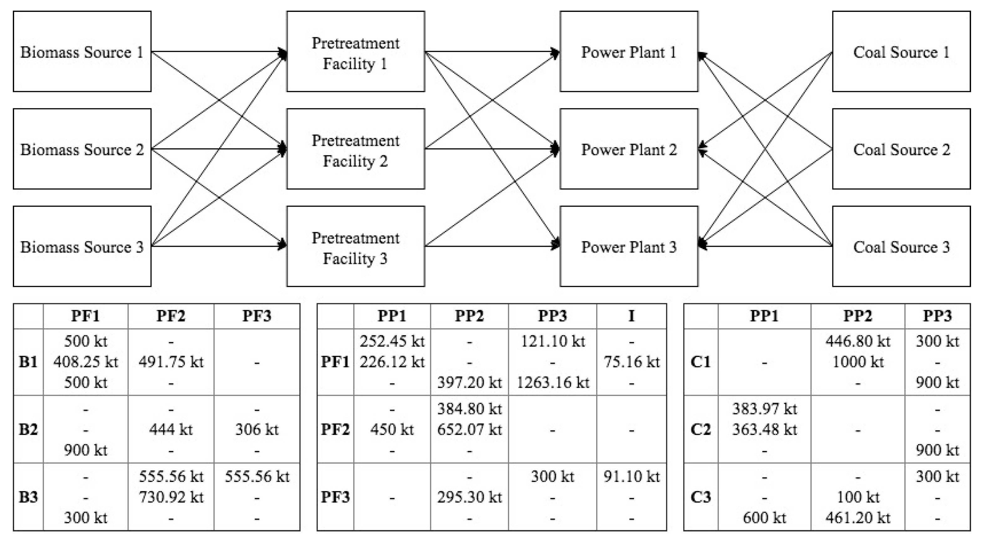
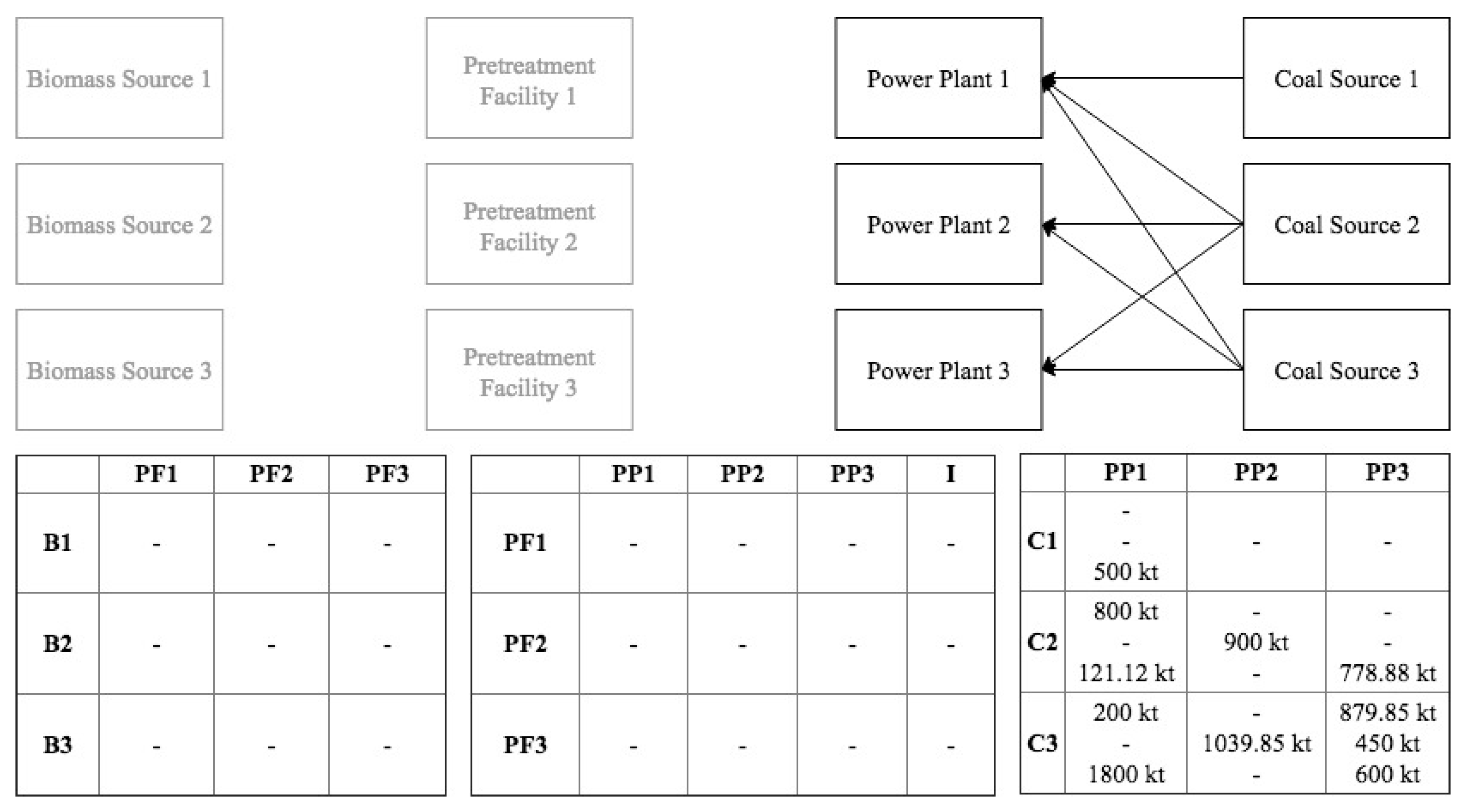
The model was implemented in General Algebraic Modelling System (GAMS) and solved using the nonlinear solver Convex Over and Under Envelopes for Nonlinear Estimation (COUENNE), with a solution time of 285.66 s and integer gap of 0.0523 on a MacBook Pro with a 3.1 GHz Intel Core i5 processor and 8 GB 2133 MHz LPDDR3 RAM. The case study considers three potential locations each for biomass sources, coal sources, pre-treatment/storage facilities, and coal power plants considered over three time periods. The biomass considered is rice straw. The resulting model has 656 continuous variables, 164 integer variables, and 425 constraints. Figure 2 illustrates the exponential increase in solution times (expressed in seconds) as the number of potential locations in each echelon is increased from 2 to 5. As the number of nodes in each echelon is increased even further, it is expected that the computation times will also increase following the same trend. Although the model seems complex, it can be easily implemented with most commercially available solvers. The data inputs required to run the model are also typically available to the user. Parameter values were used based on various literature sources.

The electricity demand and supply of biomass and coal are given in

Table 2. Supply and Demand Parameters.

	Period 1	Period 2	Period 3
Demand (MJ)	47,000	48,500	49,000
Biomass Supply (kt)
B 1	800	900	1050
B 2	1000	750	1200
B 3	1200	1050	850
Coal Supply (kt)
C 1	1550	1350	1000
C 2	800	1000	900
C 3	3000	2250	2500

. The bulk density, moisture content, and ash content of raw biomass, particularly rice straw, from each source are summarized in

Table 3. Biomass Quality Parameters.

	Bulk Density (kg/m3)			Moisture Content (% wt.)			Ash Content (% wt.)
	Period 1	Period 2	Period 3	Period 1	Period 2	Period 3	Period 1	Period 2	Period 3
B 1	50	30	55	17	18	20	17	18	20
B 2	35	40	40	25	20	19	25	20	19
B 3	60	70	55	18	23	22	18	23	22

. The higher heating value of rice straw is 18 MJ/kg. Data on rice straw properties were adapted from Liu et al. [27] and Kargbo et al. [28]. The improvement effectiveness for ash and moisture content, and resulting bulk density of each pretreatment facility are shown in

Table 4. Pretreatment Facility Characteristics.

	Ash	Moisture	Bulk Density (kg/m3)	Storage Damage Factor	Storage Capacity (kt)
PF 1	65%	35%	25	2	1350
PF 2	76%	52%	20	7	1000
PF 3	54%	67%	30	5	2250

. Table 4 also gives the amount of damage in biomass when it is stored, and the storage capacity in each pretreatment facility. The damage factor for transporting raw and pretreated biomass are 0.10 and 0.05, respectively, while moisture content increases by 0.10 due to storage. Additionally, the initial processing capacity of the pretreatment facilities is 500 kt. The displacement, ash content, and moisture content limits of each power plant are given in

Table 5. Power Plant Facility Characteristics.

	Displacement Limits (%)	Ash Content (% wt.)	Moisture Content (% wt.)
PP 1	[0, 40]	0	[10, 12]
PP 2	[0, 45]	0	[10, 12]
PP 3	[0, 40]	0	[10, 12]

. Upper and lower coal displacement limits are strictly enforced in the power plants. On the other hand, the feedstock may violate the maximum preferred ash content and allowable range for moisture content, but this would lead to negative consequences on equipment efficiency; thus, they act only as soft constraints. Input parameters for coal composition are summarized in

Table 6. Coal Quality Parameters.

Bulk Density (kg/m3)	78.5
Lower Heating Value (MJ/kg)	30
Ash Content (% wt.)	5
Moisture Content (% wt.)	9

and were adapted from Bains et al. [29]. The distances between biomass sources and pretreatment facilities, pretreatment facilities to power plants, and coal sources to power plants are shown in

Table A1. Distance between Biomass Sources and Pretreatment Facilities in km.

	PF 1	PF 2	PF 3
B 1	15	20	25
B 2	25	20	20
B 3	25	18	17

,

Table A2. Distance between Pretreatment Facilities and Power Plants in km.

	PP 1	PP 2	PP 3
PF 1	10	17	9
PF 2	15	20	15
PF 3	18	18	18

and

Table A3. Distance between Coal Sources and Power Plants in km.

	PP 1	PP 2	PP 3
C 1	15	15	15
C 2	10	15	12
C 3	15	20	18

of the Appendix A. The weight and volume capacities are 450 kt and 75 m³ respectively. Costs to purchase biomass and coal, and to retrofit each coal power plant for co-firing are given in

Table A4. Biomass and Coal Purchase Costs and Retrofitting Costs.

	B 1	B 2	B 3
Biomass Price (US$/kg)	2.5	1.75	1.5
	C 1	C 2	C 3
Coal Price (US$/kg)	3	1.75	2
	PP 1	PP 2	PP 3
Retrofitting Cost (US$)	5000	7000	4300

. Power plant associated costs are summarized in

Table A5. Power Plant Costs.

	Fixed Operating Cost (US$)			Fixed Biomass Option (US$)
	Period 1	Period 2	Period 3	Period 1	Period 2	Period 3
PP 1	350	300	350	20	24	35
PP 2	300	450	375	60	45	30
PP 3	385	375	385	35	30	45
	Biomass Combustion Cost (US$/kg)			Coal Combustion Cost (US$/kg)
	Period 1	Period 2	Period 3	Period 1	Period 2	Period 3
PP 1	2	3	1.5	2	2.25	2.5
PP 2	5	4	1	3	2.75	2.8
PP 3	4	3.5	5	2.6	2.5	3
	Fixed Expansion Costs (US$)			Unit Expansion Costs (US$/kg)
	Period 1	Period 2	Period 3	Period 1	Period 2	Period 3
PP 1	300	295	325	1	1	1
PP 2	500	375	350	1.25	1.25	1.5
PP 3	475	388	420	1.75	1.5	1

, while costs associated with processing and storing biomass in pretreatment facilities are given in

Table A6. Pretreatment Facility Costs.

	Fixed Operating Cost (US$)			Biomass Pretreatment Cost (US$/kg)
	Period 1	Period 2	Period 3	Period 1	Period 2	Period 3
PF 1	50	75	80	3	1	1.5
PF 2	80	69	78	2	2	2
PF 3	68	80	75	1.7	2.15	1.85
	Fixed Expansion Costs (US$)			Unit Expansion Costs (US$/kg)
	Period 1	Period 2	Period 3	Period 1	Period 2	Period 3
PF 1	200	350	300	1	1.25	1.5
PF 2	500	400	450	1.75	1.5	1.1
PF 3	200	375	425	1.25	1	1.35
	Fixed Holding Costs (US$)			Unit Holding Costs (US$/kg)
	Period 1	Period 2	Period 3	Period 1	Period 2	Period 3
PF 1	50	35	75	0.5	0.15	0.3
PF 2	100	65	45	0.15	0.2	0.25
PF 3	50	50	50	0.3	0.25	0.2

. Transportation costs are assumed to be US$ 18/km-kg. Lastly,

Table A7. Emissions Parameters.

Biomass Pretreatment Emissions	0.03 kg CO2/kg
Transportation Emissions	0.12 kg CO2/km
Biomass Combustion Emissions	0.08 kg CO2/kg
Coal Combustion Emissions	0.50 kg CO2/kg

summarizes the emissions from biomass pretreatment, transporting biomass, and the combustion of biomass and coal. Cost and emissions parameters were adapted from the studies of Griffin et al. [14] and Mohd Idris et al. [13] respectively.

The relationship between conversion equipment efficiency, feedstock property violations and total feedstock processed is modeled with an arbitrary function for the model validation. An exponential decay function is used as in Equation (38):

$${\lambda }_{lt}=constan{t}^{-\left(m_{lt}^{+}+m_{lt}^{-}+a_{lt}^{+}+Q_{lt}\right)}$$

(38)

Statistical experiments support that the negative exponential function may be used to describe the performance degradation of equipment. The specific behavior of degradation differs between each unit of equipment and, as a result, would have a unique combination of input parameters to accurately predict behavior. These parameters may be obtained through exponential regression [30]. An exponential decay function with a base that is between 0 to 1 will return decreasing values as the exponent variables increase. Efficiency will begin at 1 when the exponent is 0 or when no feedstock property violations have been made and/or no feedstock has been handled by the power plant yet. The efficiency value will then decrease, approaching 0 as the exponent increases. The constant dictates the rate of decrease per unit increase in the exponent variables. The higher the constant is, the faster the rate of decrease will be. As shown in Figure 3, the decrease in efficiency is more significant when the constant used is 4 compared to when the constant is equal to 2. For the purpose of validating the model, a hypothetical system is captured, and the constant for the negative exponential function was set to 2.

The results are presented in three parts, namely where each sub-objective is optimized separately, followed by the complete model run. Running the model wherein each objective is minimized individually is necessary to obtain the potential and worst values for cost and emissions needed in the full model run.

5.1. Base Case

5.1.1. Minimizing Cost

In minimizing the cost component separately, model results show a bias towards using only coal to satisfy the demand for energy as presented in Figure 4. This is because coal is relatively cheap compared to biomass, especially when considering transportation and storage requirements, pre-treatment costs, and investment costs for retrofitting existing coal power plants. Furthermore, using biomass, which are not within machine specifications, decreases conversion efficiency which then requires more feedstock to satisfy demand. However, optimizing the network based solely on minimizing costs sacrifices the environmental objective as shown in

Table 7. Comparison of costs and emissions objective performances.

	Potential	Minimizing Cost	Minimizing Emissions	Complete Model Run
					Efficiency
Cost (Million US$)	45,959.97	45,959.97	360,920.00	80,859.36	0.8892
Emissions (kt CO2)	3491.29	4858.40	3491.29	3642.78	0.8892

.

5.1.2. Minimizing Emissions

On the other hand, when the environmental objective is optimized solely, more biomass is purchased and used in all existing coal power plants to prevent incurring the much larger emissions from coal firing as shown in Figure 5. However, cost inflates significantly (Table 7) because of several reasons. Transporting biomass is relatively more expensive because of its inherent properties, in addition pre-treatment will also have associated fixed and operating costs. Without regard for costs, all the pre-treatment facilities are opened depending on the pre-treatment process and effectiveness of each facility most suited to the initial quality of the biomass. In addition, the use of more biomass results in efficiency loss in the equipment leading to the purchase of more fuel to reach demand. This is why significant increases are seen in fuel use in the second and third periods.

Optimizing each objective as single optimization models reiterate that a compromise must be found between the two conflicting objectives. One objective should not be minimized too much that no attention is given to the other. Considering only economic costs in optimizing the network result to a scheme where crucial investments and processes are disregarded to reduce costs, significantly compromising environmental sustainability. Similarly, when the system is optimized solely on environmental performance, costs are dramatically increased which may make the solution impractically expensive.

A goal programming approach is used to address this and achieve a solution that balances the two objectives. Each sub-objective–the economic and environmental–are optimized as single objective models and the results are recorded. The desirability levels of the objectives are computed for by dividing the actual improvement achieved by the potential improvement. In this case, the potential improvements for cost and environmental emissions are Million US$ 314,960.03 and 1367.1058 kt CO₂, respectively, based on the values shown in Table 7. The minimum between two efficiencies are maximized to obtain a solution that balances the minimization of costs and emissions.

5.1.3. Full Model Run

As shown in Table 7, simultaneously optimizing both objectives allow the system to reach efficiency ratings closer to each other, both objectives getting 0.8892 desirability levels. Figure 6 also show a more manageable network configuration. In an effort to control both costs and emissions, biomass is used by the system and only two pre-treatment facilities are opened. Less biomass is used compared to when only the emissions were minimized. Only two of the three coal power plants are retrofitted for co-firing. Because less biomass is used, the decrease in boiler efficiency is slower. As a result, when comparing the fuel usage of the optimal network and the network which optimized the environmental aspect only, the increase across periods is not as dramatic. Aside from this, overall fuel usage is also less because a lower biomass-to-coal blend ratio means that the lower heating value of the feedstock is higher, resulting in a higher electricity yield. In addition, only two pre-treatment facilities are chosen to avoid the additional costs needed to operate more pre-treatment facilities. This required the model to choose the facility which costs the least to operate but resulted in the best improvements in biomass properties.

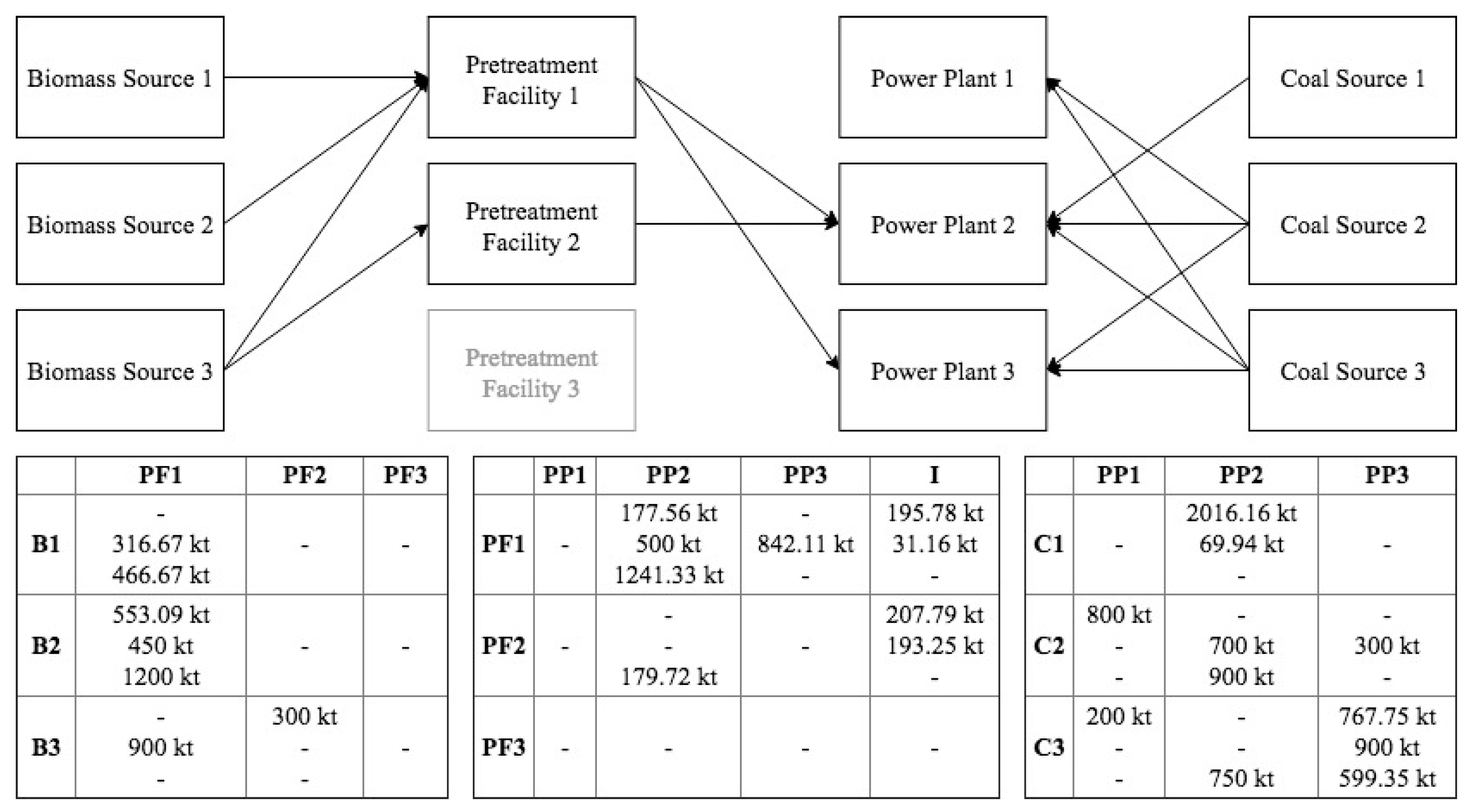
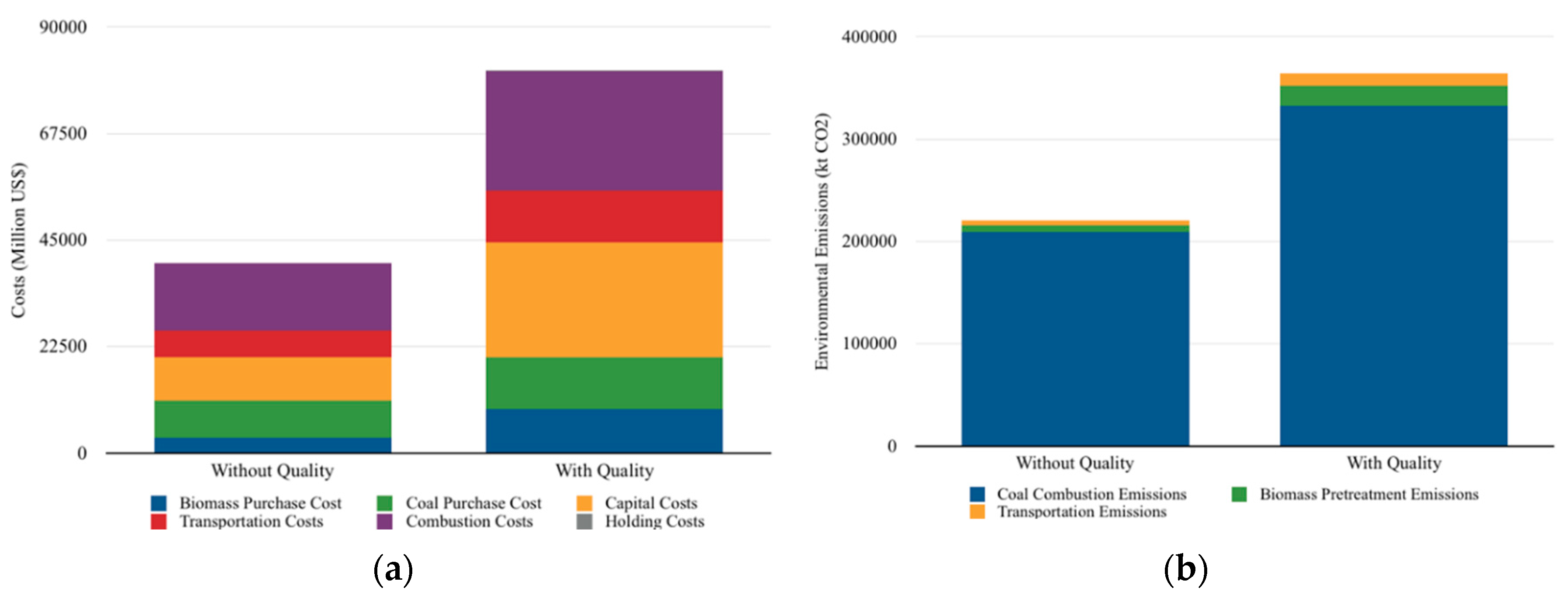
6. Scenario Analysis

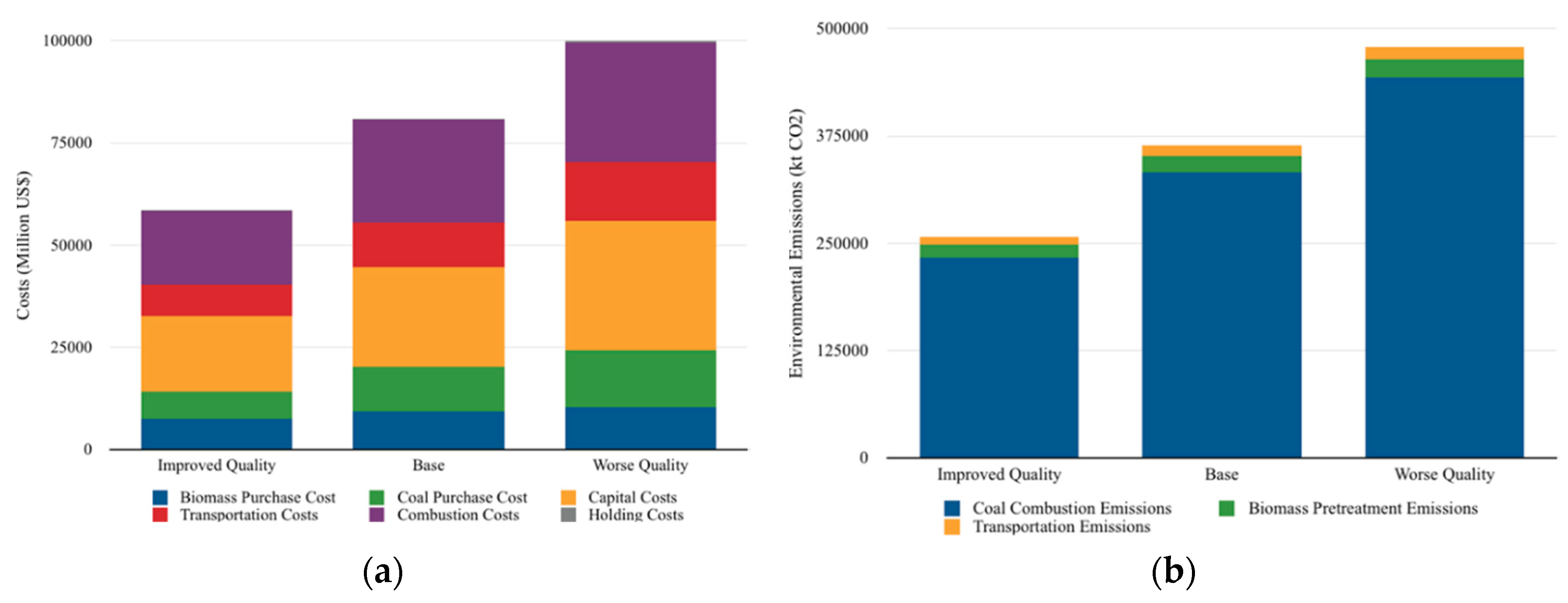
6.1. Impact of Feedstock Properties Consideration

The model was optimized without considering feedstock properties and compared to the results of the proposed model to demonstrate the impact of these considerations on a biomass co-firing supply chain, particularly on storage, transportation, and pretreatment decisions, and conversion yield. The resulting network is presented in Figure 6.

The optimized network without quality considerations (Figure 7) is compared to the optimal network obtained from the model proposed in this work (Figure 6). Without the consideration of biomass and coal properties in the network, biomass is sourced only from two locations and only two coal power plants are activated. Less fuel is used by the network because no damage occurs to the fuel during storage and transport and coal power plant conversion equipment does not experience any changes in yield or capacity. Thus, the supply and capacity of two biomass sources and two coal power plants are already enough to satisfy the demand for power in each period. Selecting where to source biomass is based only on distance and costs, unlike in the proposed model where the properties of the biomass from each source is also a factor in this decision. Similarly, pretreatment facilities/processes are chosen based on distance and pretreatment costs instead of their effectiveness in improving the qualities of the biomass. The amount of inventory held across periods is reduced also because the cost of purchasing and pretreating biomass remains relatively stable, so there is no need to keep inventory. On the other hand, the proposed model chooses to hold inventory on certain periods to avoid periods where the quality of the biomass is worse. In addition, only one of the two active coal power plants are retrofitted for co-firing. The system becomes less careful with distributing the amount of biomass usage among coal power plants, as it no longer has to avoid possible deterioration in conversion equipment and variations in the lower heating value of the mixed fuel. As such, in an effort to reduce transport and retrofitting costs, as well as transport emissions, biomass is only transported and used in one of the two active coal power plants. The model which overlooks quality related issues also has significantly lower costs (Million US$ 40,150.17) and emissions (2209.40 kt CO₂). The graphs in Figure 8a,b illustrate the components of costs and emissions for both optimized models.

Without considering biomass quality, costs are lowered in all of its components–purchase, transport, pretreatment, combustion, holding, and capital costs. As explained earlier, this is because of the significantly decreased fuel that flows through the system. Transportation costs are also decreased because the bulk density of the biomass and coal are not accounted for, which entail difficulties in transporting material (e.g., requiring additional trips). Similarly, emissions are considerably lower in this scenario because of the same reasons.

Although this scenario achieved better performance for the financial and environmental objectives, it is an inaccurate and unreliable model of a biomass co-firing network, and will not be useful as a planning or management tool.

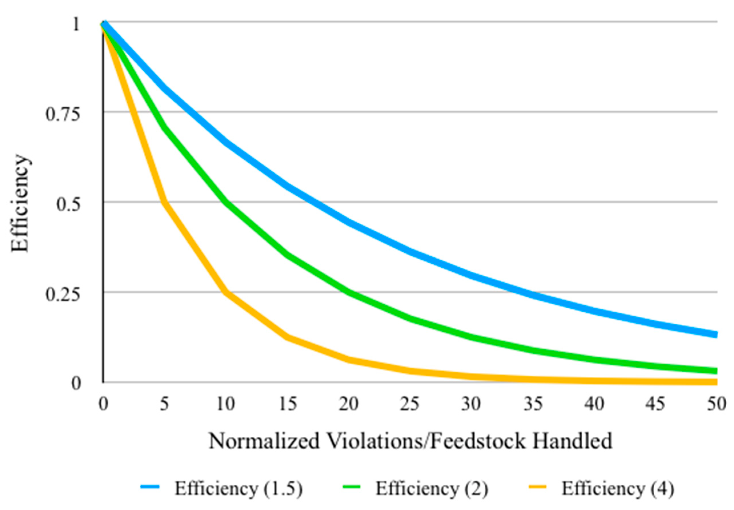
6.2. Biomass Properties

Biomass properties show to be a significant consideration in the modelling of biomass supply chains because it influenced network decisions across all activities in the supply chain. Changes in the properties of the biomass may cause an impact in the way the biomass co-firing network is constructed, consequently affecting the network’s financial and environmental sustainability.

The biomass properties were improved and worsened across all periods in two different scenarios and are compared with the base scenario. In the improved properties scenario, moisture content and ash content are decreased by 20%, while bulk density is increased by 20%. On the other hand, biomass properties are worsened by increasing moisture content and ash content by 20%, and reducing bulk density by 20%. The cost and environmental emissions performance for the two scenarios and the baseline scenario are shown in Figure 9.

It can be observed that costs and emissions increase as the properties of biomass worsen. The improved properties scenario yielded the least cost and environmental emissions, while the worsened properties scenario resulted in higher costs and emissions.

The breakdown of costs is analysed in Figure 9a to understand why costs increased as properties worsened. With worse biomass quality, efficiency loss experienced by the conversion equipment in coal power plants also worsen, requiring the system to purchase and use more fuel. This increases all cost components, such as fuel purchase costs, transport, pre-treatment, and combustion costs. Transportation costs also increase because of the worse bulk density of the biomass, requiring multiple deliveries. On the other hand, as properties improved, the system would have to rely on less fuel overall because the power plants experience less loss in efficiency. Thus, less biomass and coal are used to reach the required amount of electricity. However, it is noticeable that when properties are worsened, biomass purchase increases only slightly, while the increase in coal purchase is more pronounced. This is because the model attempts to control the damage biomass causes on the conversion equipment and the additional costs needed to handle biomass by diluting biomass properties with more desirable coal properties.

Likewise, Figure 9b also shows an overall increase in environmental emissions as biomass properties worsen. For similar reasons, all components of environmental emissions increase due to the need to process more fuel. Combustion emissions due to coal increases because the model chooses between the corrosion in boiler equipment, which will require additional fuel and cause harmful emissions, and the emissions from burning coal.

Another set of scenarios are analysed. Particularly, a scenario wherein biomass properties are worsened only in the second period and where properties are improved only in the second period. The properties are enhanced and worsened by 50% from their original value.

When biomass properties are relatively stable across periods, storage of the biomass is avoided because it damages the biomass. However, when biomass properties experience increased moisture content, for example during wet season, and increased ash content, purchases are done during earlier periods with sufficient quantity and appropriate quality and stored for future use. When moisture content and ash content were higher and bulk density was lower in the second period, purchase during this period decreased significantly. Instead, the biomass to be used on the second period were purchased during the first and stored. The additional amount purchased in period 1 allotted an extra amount to account for deterioration and loss due to transport and storage. As a result, purchase, transport, and pre-treatment costs and emissions increase because of the additional biomass purchased in period 1, holding costs also increase to store biomass. Changes to combustion costs and emissions, as well as the efficiency loss experienced by the equipment are negligible because the original properties in period 2 are only slightly different from period 1. The optimal network for this scenario is shown in Figure 10. In the same way, when the properties in period 2 are made significantly better relative to period 3, the model chooses to purchase biomass for period 3 during the second period (Figure 11).

7. Conclusions

A MINLP model for optimizing a biomass co-firing supply chain network has been developed, which integrates feedstock properties considerations while simultaneously minimizing economic costs and environmental emissions through goal programming. This model incorporates the impact of feedstock, transportation, and pre-treatment requirements. Changes in biomass properties as it moves through the network are accounted for, together with the impact of feedstock properties on conversion yield and equipment degradation. The inclusion of these in the model showed to be an important enhancement to traditional models because decisions on how much and when to source biomass and coal, and the use of pretreatment facilities, storage, and combustion in coal power plants were considerably affected by the said considerations.

Minimizing either the financial or environmental objective individually emphasized the conflicting nature of the two objectives. Simultaneously optimizing both objectives created a network which balanced performance on both objectives.

It was also shown that without considerations for feedstock properties, costs and emissions were artificially decreased, leading to the purchase of insufficient fuel and combustion of inappropriate fuel which may result in damage or loss in efficiency of the equipment. Hence, the model proposed in this study is a better fit to design and manage a biomass co-firing network.

Extensions on this research may consider biomass quality and availability as uncertain parameters in a robust multi-objective optimization model. Precise data regarding the quality of the feedstock is not readily available, and any error in estimation requires operational adjustments to be made. As feedstock quality has been proven to be an important inclusion in biomass co-firing networks, these networks should be made robust to such uncertainties. Additionally, this study assumes that the network’s nodes are all functional and benign; however, in reality, the presence of faulty and uncooperative components must be considered [31]. Lastly, the parameters used in the validation of the proposed model may be considered too optimistic and difficult to match in real market. Thus, the application of the model to real-world problems may be explored, along with efficient solution strategies for the resulting large-scale problems.

References

1. International Energy Outlook. 2017; (DOE/EIA-0484(2017)). Available online: https://www.eia.gov/outlooks/ieo/pdf/0484(2017).pdf (accessed on 23 September 2018).
2. Iakovou, E.; Karagiannidis, A.; Vlachos, D.; Toka, A.; Malamakis, A. Waste biomass-to-energy supply chain management: A critical synthesis. Waste Manag. 2010, 30, 1860–1870. [Google Scholar] [CrossRef] [PubMed]
3. Ramos, A.; Monteiro, E.; Silva, V.; Rouboa, A. Co-gasification and recent developments on waste-to-energy conversion: A review. Renew. Sustain. Energy Rev. 2018, 81, 380–398. [Google Scholar] [CrossRef]
4. Dundar, B.; McGarvey, R.G.; Aguilar, F.X. Identifying Optimal Multi-state collaborations for reducing CO2 emissions by co-firing biomass in coal-burning power plants. Comp. Ind. Eng. 2016, 101, 403–415. [Google Scholar] [CrossRef]
5. Madanayake, B.N.; Gan, S.; Eastwick, C.; Ng, H.K. Biomass as an energy source in coal co-firing and its feasibility enhancement via pre-treatment techniques. Fuel Process. Technol. 2017, 159, 287–305. [Google Scholar] [CrossRef]
6. Mauro, C.; Rentizelas, A.A.; Chinese, D. International vs. domestic bioenergy supply chains for co-firing plants: The role of pre-treatment technologies. Renew. Energy 2018, 119, 712–730. [Google Scholar] [CrossRef] [Green Version]
7. Zandi Atashbar, N.; Labadie, N.; Prins, C. Modeling and optimization of biomass supply chains: A review and a critical look. IFAC-PapersOnLine 2016, 49, 604–615. [Google Scholar] [CrossRef]
8. Shafie, S.; Mahlia, T.; Masjuki, H. Life cycle assessment of rice straw co-firing with coal power generation in Malaysia. Energy 2013, 57, 284–294. [Google Scholar] [CrossRef]
9. Oanh, N.T.K.; Tipayarom, A.; Bich, T.L.; Tipayarom, D.; Simpson, C.D.; Hardie, D.; Liu, L.J.S. Characterization of gaseous and semi-volatile organic compounds emitted from field burning of rice straw. Atmos. Environ. 2015, 119, 182–191. [Google Scholar] [CrossRef]
10. Ba, B.H.; Prins, C.; Prodhon, C. Models for optimization and performance evaluation of biomass supply chains: An Operations Research perspective. Renew. Energy 2016, 87, 977–989. [Google Scholar] [CrossRef]
11. Shang, Y.L. Optimal control strategies for virus spreading in inhomogeneous epidemic dynamics. Canad. Math. Bull. 2013, 56, 621–629. [Google Scholar] [CrossRef]
12. Pérez-Fortes, M.; Laínez-Aguirre, J.M.; Bojarski, A.D.; Puigjaner, L. Optimization of pre-treatment selection for the use of woody waste in co-combustion plants. Chem. Eng. Res. Des. 2014, 92, 1539–1562. [Google Scholar] [CrossRef]
13. Mohd Idris, M.N.; Hashim, H.; Razak, N.H. Spatial optimisation of oil palm biomass co-firing for emissions reduction in coal-fired power plant. J. Clean. Prod. 2018, 172, 3428–3447. [Google Scholar] [CrossRef]
14. Griffin, W.; Michalek, J.; Matthews, H.; Hassan, M. Availability of Biomass Residues for Co-Firing in Peninsular Malaysia: Implications for Cost and GHG Emissions in the Electricity Sector. Energies 2014, 7, 804–823. [Google Scholar] [CrossRef] [Green Version]
15. Savic, D. Single-objective vs. Multiobjective Optimisation for Integrated Decision Support. In Proceedings of the 9th International Congress on Environmental Modelling and Software, Lugano, Switzerland, 24–27 June 2002; Volume 119, pp. 7–12. [Google Scholar]
16. Rollan, C.D.; Li, R.; San Juan, J.L.; Dizon, L.; Ong, K.B. A planning tool for tree species selection and planting schedule in forestation projects considering environmental and socio-economic benefits. J. Environ. Manag. 2018, 206, 319–329. [Google Scholar] [CrossRef] [PubMed]
17. Ramos, M.; Boix, M.; Montastruc, L.; Domenech, S. Multiobjective Optimization Using Goal Programming for Industrial Water Network Design. Ind. Eng. Chem. Res. Am. Chem. Soc. 2014, 53, 17722–17735. [Google Scholar] [CrossRef] [Green Version]
18. Malladi, K.T.; Sowlati, T. Biomass logistics: A review of important features, optimization modeling and the new trends. Renew. Sustain. Energy Rev. 2018, 94, 587–599. [Google Scholar] [CrossRef]
19. Castillo-Villar, K.K.; Eksioglu, S.; Taherkhorsandi, M. Integrating biomass quality variability in stochastic supply chain modeling and optimization for large-scale biofuel production. J. Clean. Prod. 2017, 149, 904–918. [Google Scholar] [CrossRef] [Green Version]
20. Boundy, R.G.; Diegel, S.W.; Wright, L.L.; Davis, S.C. Biomass Energy Data Book; Oak Ridge National Laboratory: Oak Ridge, TN, USA, 2011. [Google Scholar]
21. Veijonen, K.; Järvinen, T.; Alakangas, E.; VTT Processes. Biomass Co-firing—An Efficient Way to Reduce Greenhouse Gas Emissions; European Bioenergy Networks: Jyväskylä, Finland, 2003. [Google Scholar]
22. Liu, Z.; Johnson, T.G.; Altman, I. The moderating role of biomass availability in biopower co-firing—A sensitivity analysis. J. Clean. Prod. 2016, 135, 523–532. [Google Scholar] [CrossRef]
23. Shang, Y.L. Resilient Multiscale Coordination Control against Adversarial Nodes. Energies 2018, 11, 1844. [Google Scholar] [CrossRef]
24. Shang, Y.L. Unveiling robustness and heterogeneity through percolation triggered by random-link breakdown. Phys. Rev. E 2014, 90. [Google Scholar] [CrossRef]
25. Hernández, J.J.; Lapuerta, M.; Monedero, E.; Pazo, A. Biomass quality control in power plants: Technical and economical implications. Renew. Energy 2018, 115, 908–916. [Google Scholar] [CrossRef]
26. Munby, D. The Assessment of Priorities in Public Expenditure. Political Q. 1968, 39, 375–383. [Google Scholar] [CrossRef]
27. Liu, Z.; Xu, A.; Zhao, T. Energy from Combustion of Rice Straw: Status and Challenges to China. Energy Power Eng. 2011, 3, 325–331. [Google Scholar] [CrossRef] [Green Version]
28. Kargbo, F.R.; Xing, J.; Zhang, Y. Property analysis and pretreatment of rice straw for energy use in grain drying: A review. Agric. Biol. J. N. Am. 2010, 1, 195–200. [Google Scholar] [CrossRef]
29. Bains, M.; Robinson, L. Material Comparators for End-of-Waste Decisions—Materials for Fuels: Coal; Environmental Agency: Bristol, UK, 2016. [Google Scholar]
30. Dai, W.; Chi, Y.; Lu, Z.; Wang, M.; Zhao, Y. Research on Reliability Assessment of Mechanical Equipment Based on the Performance-Feature Model. Appl. Sci. 2018, 8, 1619. [Google Scholar] [CrossRef]
31. Shang, Y.L. Localized recovery of complex networks against failure. Sci. Rep. 2016, 6. [Google Scholar] [CrossRef] [PubMed]
Figure 1. Network superstructure.
Energies 12 02252 g001
Figure 2. Solution Time of Varying Model Sizes.
Energies 12 02252 g002
Figure 3. Conversion Efficiency Function Graphs.
Energies 12 02252 g003
Figure 4. Minimum Cost Network.
Energies 12 02252 g004
Figure 5. Minimum Environmental Emissions Network.
Energies 12 02252 g005
Figure 6. Optimal Biomass Co-firing Network.
Energies 12 02252 g006
Figure 7. Optimal Biomass Co-firing Network without Quality Considerations.
Energies 12 02252 g007
Figure 8. Breakdown of (a) costs and (b) environmental with and without Quality Considerations.
Energies 12 02252 g008
Figure 9. Breakdown of (a) costs and (b) environmental when Biomass Properties are Varied.
Energies 12 02252 g009
Figure 10. Optimal Network for Worse Biomass Properties in Period 2.
Energies 12 02252 g010
Figure 11. Optimal Network for Improved Biomass Properties in Period 2.
Energies 12 02252 g011