Optimization of Cooling Utility System with Continuous Self-Learning Performance Models
by
 ,
,
Ron-Hendrik Peesel
1,* ,
,
Florian Schlosser
1,
Henning Meschede
1,
Heiko Dunkelberg
1 and
Timothy G. Walmsley
2 1
Department for Sustainable Products and Processes (upp), University of Kassel, 34125 Kassel, Germany
2
Sustainable Process Integration Laboratory—SPIL, NETME Centre, Faculty of Mechanical Engineering, Brno University of Technology—VUT Brno, Technická 2896/2, 616 69 Brno, Czech Republic
*
Author to whom correspondence should be addressed.
Energies 2019, 12(10), 1926; https://doi.org/10.3390/en12101926
Submission received: 17 April 2019
/
Revised: 10 May 2019
/
Accepted: 16 May 2019
/
Published: 20 May 2019
(This article belongs to the Special Issue Selected Papers from PRES 2018: The 21st Conference on Process Integration, Modelling and Optimisation for Energy Saving and Pollution Reduction)
Abstract
:Prerequisite for an efficient cooling energy system is the knowledge and optimal combination of different operating conditions of individual compression and free cooling chillers. The performance of cooling systems depends on their part-load performance and their condensing temperature, which are often not continuously measured. Recorded energy data remain unused, and manufacturers’ data differ from the real performance. For this purpose, manufacturer and real data are combined and continuously adapted to form part-load chiller models. This study applied a predictive optimization algorithm to calculate the optimal operating conditions of multiple chillers. A sprinkler tank offers the opportunity to store cold-water for later utilization. This potential is used to show the load shifting potential of the cooling system by using a variable electricity price as an input variable to the optimization. The set points from the optimization have been continuously adjusted throughout a dynamic simulation. A case study of a plastic processing company evaluates different scenarios against the status quo. Applying an optimal chiller sequencing and charging strategy of a sprinkler tank leads to electrical energy savings of up to 43%. Purchasing electricity on the EPEX SPOT market leads to additional costs savings of up to 17%. The total energy savings highly depend on the weather conditions and the prediction horizon.

1. Introduction
Generation of cold utility for industrial processes consumes about 9% of the net electricity in Germany, with similar trends in other countries, and an overall chiller energy efficiency ratio (EER) of less than two [1]. Cold utility systems encompass cooling towers (evaporative coolers), air coolers, and refrigeration. Air coolers incur near-zero running costs (i.e., “free cooling chiller”), cooling towers require water make-up and chemicals, while refrigeration is normally driven by electricity with substantial running expenses that are approximately one order of magnitude higher than a cooling tower system. Maximizing the use of the lowest-cost utility saves running costs and high-quality energy, reducing environmental burdens. The ongoing digitization of many processes in the industry enables the potential to automate and optimize the operation of cold utility units. Coupled with an efficient and flexible utility system, a site can achieve substantially highier levels of system efficiency. Critical to this vision is linking sectors—e.g., process heating and cooling and electricity grid—combined with technologies, processes, and control systems to collect and analyze the data and implement complex energy optimization methods. Prerequisite for an efficient cooling system is the knowledge and the optimal combination of different operating and performance conditions of individual chillers. The performance of cooling systems depends on their part-load performance and their condensing temperature, which are often overlooked and not continuously measured. Manufacturer performance data often substantially differ from in-plant performance [2].
The optimized operation of refrigeration units in combination with a complex control algorithm can improve the energy efficiency of cooling systems when implemented. Clausen et al. [3] show that the coupling of optimization and simulation of parcel sorting plants lead to efficiency increases. Dynamic simulations support both the validation of efficiency concepts prior to implementation and model-based optimization. Augenstein [4] discusses that a linear optimization of the chiller deployment strategy reduces power consumption by 11%. At the same time, there is also optimization potential for specifically adapted expert control strategies in the sequencing of refrigeration systems. Rule-based controls show a good performance for specific systems under normal conditions [5]. Changes in boundary conditions lead to nonlinear behavior of equipment, and equipment degradation can shift the optimum operating set-points and control of a plant over its life cycle [6].
Several approaches are reported in the literature to optimize cooling system operations. Hovgaard et al. [7] use the example of a supermarket refrigeration supply to show that electrical energy savings of 9%–32% are possible with the help of model predictive control (MPC) with a thermal storage system, predicting the changing load and taking into account varying energy prices. Braun [8] reduced the energy consumption with a component-based and system-based optimization algorithm and correlated the power consumption of the chillers, condenser pump, and cooling tower fans with a quadratic function. Olson et al. [9] describe a mathematical approach to the distribution of loads over several chillers to minimize energy costs. Many different methods for optimal chiller sequencing control have been investigated. Some examples are the branch-and-bound method [10] dynamic programming [11], gradient method [12], genetic algorithms [13], simulated annealing [14], and the particle swarm optimization [15]. These methods generally perform well in a simulation environment.
One of the challenges with practical implementation is system dynamics leading to exponentially increased computational demand. To reduce computing time for dynamic optimization, Powell et al. split up the problem solving into a dynamic one for the total load at each time step and a static one for the optimal chiller loading. For a 24 h time horizon, the energy savings are around 9.4% and the energy costs savings are 17.4%. [16] A literature review reveals that the energy-saving potential varies between 5% [17] and 40% [18] depending on the case study.
Another important factor is the availability of cold storage for a cooling system. Kapoor et al. [19] show that implementing a 15,000 m³ cold-water storage tank could result in a cost saving of 13%. Cold energy storage presents an opportunity to reduce costs by shifting loads. Cole et al. [20] use an MPC with thermal energy storage and variable electricity prices for peak and off-peak hours to reduce the electrical energy consumption and the operating costs for the cooling system of one building. In the best case, the annual costs are reduced by around 42% while the total energy usage increases by more than 6%. Kircher and Zhang [21] investigate the cooling strategy of an office building with ice and chilled water storages using an MPC and demand response incentives. The optimization horizon is limited to one day, and the non-linear part-load performance of the chillers is neglected. Ma et al. [22] show that an MPC implementation for a building cooling system considering a storage tank, cooling towers, condensing, and evaporation temperature increases the plant coefficient of performance (COP) by around 19%. A direct charging and discharging of the storage by the cooling tower is not analyzed. With a similar idea to the current study, Soler et al. [23] present a performance optimization of a district cooling network with eight chillers and a thermal storage tank for a one day period, assuming the use of chillers according to their efficiency rating and best performance in full load. For minimizing shut-downs and start-ups, no-increase/no-decrease constraints are added.
Many production sites use cold-water storage tanks to smooth the cooling load profile but not for load management and load shifting. A sprinkler tank contains a high volume of water for use in emergencies such as extinguishing fires. There is an opportunity to utilize the sprinkler tank for cold-water storage with load shifting while maintaining a minimum water level for emergency operations. Using a free cooling chiller (i.e., cooling by air or cooling water from a cooling tower) offers the opportunity to provide cold water with a higher energy efficiency compared to a compression chilling machine. However, if ambient temperatures equal or exceed the cold water set point temperature, the free cooling chiller is no longer effective. Extending the operation hours of the free cooling chiller and reducing compression chiller’s could save a significant amount of electrical energy. This needs a complex pre-charge and discharge control for the cold-water storages. To this end, a mixed integer linear optimization (MILP) algorithm is advantageous.
In practical applications, the performance is highly dependent on the accuracy of the performance models and the effectiveness of the convergence of the optimization algorithm. As demonstrated in the literature review, a current gap is a lack of properly accounting for in-plant chiller performance and considerations for how performance changes through its lifetime. This weakness can be compensated by implementing continuous self-learning performance models and linking the optimization algorithm and dynamic simulations including part-load (off-design).
The aim of this study is to develop and apply a predictive optimization algorithm for multiple compression chillers, a free cooling chiller, and a sprinkler tank as a cold-water storage tank considering part-load system operation under a dynamic simulation to improve overall energy cost efficiency. The algorithm extends the work of Peesel et al. [2], who introduced a predictive simulation-based optimization for a food processing factory, calculating electricity savings of up to 23% per year. The novelty of this study is the evaluation of the interdependency between part-load ratio, variable electricity prices, and a sprinkler tank using data from an industrial energy monitoring system. Furthermore, the influence of the prediction horizon and the ambient temperature on the optimization result is evaluated. The modeling of the utilities, the load profile of cold water, and the framework conditions are based on the energy data of a plastics processing company. For the performance curves of the utility, a continuous self-learning model is used. Additionally, the initial states of the optimization are reset by the simulation results of the previous timestep. The combination of the linear optimization and the dynamic simulation gains the advantages of both methods. This results in more realistic and accurate results for the energy and costs-saving potential of the predictive simulation-based optimization. The developed optimization algorithm is applied to case studies of plastic manufacturers in Germany and Spain to demonstrate its potential.
The remainder of the article is structured as follows. Section 2 presents the general approach of the optimization, the data pre-processing, modeling of the performance curve, and the simulation model. The case study of a plastic processing company is introduced in Section 3. This is followed by the explanation of the results, including the influences of the prediction time horizon, ambient temperature, and variable electricity price, in Section 4. The conclusion is presented in Section 5 together with an outlook for further research.
2. Method and Simulation Model
This section describes the overall method and simulation modeling approach of the systems using a model-based predictive optimization considering the individual operating performance of the refrigeration supply system by continuously self-learning performance curve models. Figure 1 shows the general optimization method with the energy data from an industrial plant and the self-learning performance curve models. The scheme of the simulation-based optimization is also visualised. The method extends the work of Peesel et al. [24] and comprises four steps. The first step includes collection and pre-processing of the data. The input conditions include the ambient temperature, the residual load, and the electricity price for the production site. At this point, a forecasting model for the weather or the cooling load can be integrated. Weather forecasts are common, whereas load forecasting has been attempted, for example, by statistical methods [25], artificial neural networks [26], and support-vector machines [27]. The energy monitoring system collects the operating data of the cold utility system for all production states. The second step is the modeling of the continuous self-learning performance models for the utilities. This is followed by the predictive optimization for the sequencing of the different chillers. The last step is the simulation of the complete utility system. The different steps are explained in more details in the subsequent subsections.
2.1. Data Pre-Processing
Energy and performance data of an energy monitoring system often contain some obvious outliers and incorrect values. This requires pre-processing the data to remove these unusable values and extract the reliable data, such as for cold water temperature (Tcold), condensing temperature (Tcond), part-load ratio (PLR), energy efficiency ratio (EER), electrical power (Pel), and thermal energy flow (). The definition of the EER and the PLR are defined by Equations (1) and (2).
The data pre-processing is split into two steps—data preparation based on system behavior and the application of statistical methods. The binary operating state is the variable that helps filter data for times, such as when plants are shut-down. These are up to 50% of all values, depending on the time span of the data such as weekly, monthly, or annual data records. Data during plant shut-downs measure electrical power values <1 kW for the chillers in standby, while cooling load data are often erroneous due to thermal inertia in the fluid. By including these data in the characteristic curve generation, an extremely high EER value results that misrepresents the actual situation. A physical method to remove outliers of the EER is the comparison of the ERR calculated from the measurement data with half of the ideal Carnot efficiency. Other important logical criteria are both the chillers’ total electrical power consumption and their transferred cooling capacity. Measured values for these variables must not assume negative values and be lower than the nominal electrical power and cooling capacity at the lowest condensing temperature stated by the manufacturer.
Statistical methods are used to identify incorrect values that pass through the analysis of system behavior. The filtering of values is performed for values smaller than a percentile (1% or 5%) or greater than a given percentile from 95% or 99%. This method is also applied to the rate of change of the recorded measurements to filter out extreme changes, especially for values of the electrical power. A special method is a classification from the minimum to the maximum condensing temperature into one Kelvin class. For this transformation, a matrix approach is used. The direction vector with the largest standard deviation is determined for each classified data matrix for PLR and EER. Outliers are determined in linear or non-linear data point distributions. The vector of the largest scatter indicates a transformed coordinate system for the size pairs of EER and PLR. In this coordinate system, further outliers are identified by the interquartile distance (IQR). In statistical studies, 1.5 times the IQR is often used to identify outliers. The analysis of energy monitoring data of six different compression chillers in three sites by the authors shows that this must be selected much smaller to filter out data. In this work, 0.5 times the IQR is used. The distribution of the data points in the respective classes is decisive for filtering out the values. The various methods are run through one after the other, starting with the method that takes the least time to calculate and filters out the most values. The order is important to minimize the total computation time. After the data pre-processing, the scattering and the number of large outliers for different measured variables were considerably reduced, shifting the median mainly due to the removal of the measured data in the switched off state. The change in the measured values after data pre-processing is shown in the following Figure 2.
2.2. Continuous Self-Learning Performance Modeling
After the data pre-processing, the modeling of the load performance curve models is performed. For the free cooling chiller, a second order linear regression model is used. Since the data pre-processing shows that measurement data are available in sufficient quantity and for all operating states, only interpolations are necessary. The following Equation (3) with the regression coefficients Bx defines the model:
The EERFC of the free cooling chiller is dependent on the PLR and the ambient temperature () for a fixed cold-water supply temperature. For the optimization, the semi-empirical regression chiller model—the Gordon–Ng universal model [28]—based on the evaporator outlet water temperature is used. Equation (4) presents the Gordon–Ng model,
where A0, A1, A2 are regression coefficients and is the cooling load of the chiller. In this study, the cold-water temperature (Tcold) is kept constant. is the ingoing condensing temperature of the compression chiller.
Former studies show that even two structurally identical compression chillers can perform differently in the same location [29]. This results in a need for empirical models for each utility operation. In operating areas with a significant quantity of energy data, empirical models describe the system performance. In other areas, extrapolating semi-empirical models is more accurate. The linking of physical and empirical modeling ensures an acceptable accuracy in both fields of interpolating and extrapolating. For the modeling of the utility, manufacturer and performance data are combined and continuously adapted to form part-load performance curve models. The existing and new data points are weighted differently in the continuous self-learning model. In considering changes in utility performance, recent data are weighted higher. If the characteristic curves are regularly adjusted over a longer period, the deviation between the previous and new characteristic curve decreases. The disadvantage of this method is that an irregularity in the measurement system or in the utilities leads to significant deviations.
For the validation of the Gordon–Ng universal model, the dataset of 1652 data points is split into a training set (82%) and a validation set (18%). The overall deviation of the EER is 8.3% and the root-mean-square error (RMSE) is 0.355. This is because of a low quantity of data for low and high PLR values. Lee et al. [30] show slightly lower values for the validation of the Gordon–Ng universal model.
2.3. Mathematical Model
The optimization is formulated as a mixed-integer linear programming (MILP) problem. Since the control parameters of the chillers are discrete, the solutions must be integers. The goal of the optimization is to satisfy the cold-water demand by multiple chilling systems for the next NT timesteps at the lowest energy costs. The sprinkler tank offers the opportunity to store cold water. This potential is used to show the load shifting potential of the cooling system by using a variable electricity price as an input parameter of the optimization. The following equations describe the minimization problem.
The different part-load operating states (St) are between 0% and 100%, while the smallest step size is 1%. The active chilling machines set the lower bound of the operating states and the step size. The cost term includes the costs for each part-load operating state (St) of the chillers. The costs are calculated by multiplying the electrical power consumption of the chiller by the electricity costs for the current time step. The electrical power consumption is based on the regression models—Equation (3) or (4). The number of chillers is defined by Ncc. The number of timesteps (NT) describes the prediction horizon of the optimization in hours. For example, an NT of 3 by a step size of 3600 s means that the optimal load distribution is found for the sum of loads of the current hour and the following two hours. In this paper, the prediction horizon is varied between 6 and 48 timesteps. Additionally, the starting costs (SC) consider the extra energy demand when starting a machine. SC also helps to prevent an unnecessary starting and stopping of the machines if the gain in efficiency is very low. The active states of the chillers are described by Xt,n,st, while Zt,n is the binary on/off-variable.
Equations (7) and (8) describe the constraints for the lower and upper bounds of the optimization. The total cooling supply by the chillers must be lower or equal to the total cooling demand of all timesteps () and the cooling capacity of the sprinkler tank (). CC is the cooling capacity of the chillers. The cooling capacity of the sprinkler tank is defined by the product of the mass of water (m) at the cold water return temperature , the specific heat capacity of water and the temperature difference of the cold water and returning water . The current potential cooling energy of sprinkler tank is calculated analogously. By varying the mass of water at the different temperatures, the cooling capacity of the thermal storage can be changed. Additionally, the total supply cannot be lower than the total cooling demand minus the current cooling power of the sprinkler tank. For solving the mixed-integer problem, the Gurobi Optimization 8.1 software is used [31].
2.4. Simulation Model
The results of the optimization are the control parameters for each chilling machine in the current timestep. These parameters represent the operating schedule for the simulation. A dynamic simulation continuously validates the set points in the optimization based on the response and feedback effects from the system. These include thermal inertia of the cooling system, start-up characteristics, as well as the physically modeled heat losses of the storage tank. There is also a difference in the start-up characteristics for a compression chilling machine in the optimization and the simulation. In the optimization, the full cooling capacity of the chiller is immediately available due to the linear programming, whereas, in the simulation, the chiller needs a few minutes to ramp to full capacity. This is modeled by a first-order delay element. Comprehensive measurements have shown that the ramp time can vary from one to five minutes or even longer for larger machines. During starting time, the cooling capacity and the energy efficiency of the compression chillers is reduced according to the part-load of the load performance curve. For part-load values below 20% of the full capacity, the EER is below two. This compensates overestimated EER by the linear programming and integrates lower efficiency in starting and shutting down times in the simulation. Therefore, the simulation compensates the limitation of the linear optimization and verifies the operating schedule. Additionally, the complex heat loss mechanisms of a storage tank are modeled more accurately in a simulation than in the linear model. The applied storage model uses the Multi-Node model of the Matlab/Simulink® CARNOT Blockset. [32] For the calculation of the Multi-Node storage model, the storage volume is divided along its height into n nodes. In each layer, an ideal mixing is assumed, i.e., the temperature is constant in the layer element in both the radial and vertical directions. For each layer and each simulation time step, the balance equation, Equation (11), of the energy transport is solved according to the first law of thermodynamics.
The change in the internal energy, U, describes the change in the temperature, T, of the individual layers as a function of entering and leaving enthalpy streams caused by the piston flow in the tank and charging mass flows, direct vertical heat conduction effects through the layers, and the heat losses through the container wall. To reduce computational time, the nodes in the model are limited to two—one for the cold-water supply temperature and one for the cold water return temperature.
This method eliminates unrealistic starting points. The initial states of the optimization are reset by the simulation results of the previous timestep. The combination of the linear optimization and the dynamic simulation enables the advantages of both methods. This results in more realistic and accurate results for the energy and costs saving potential of the predictive simulation-based optimization.
3. Plastic Processing Case Study
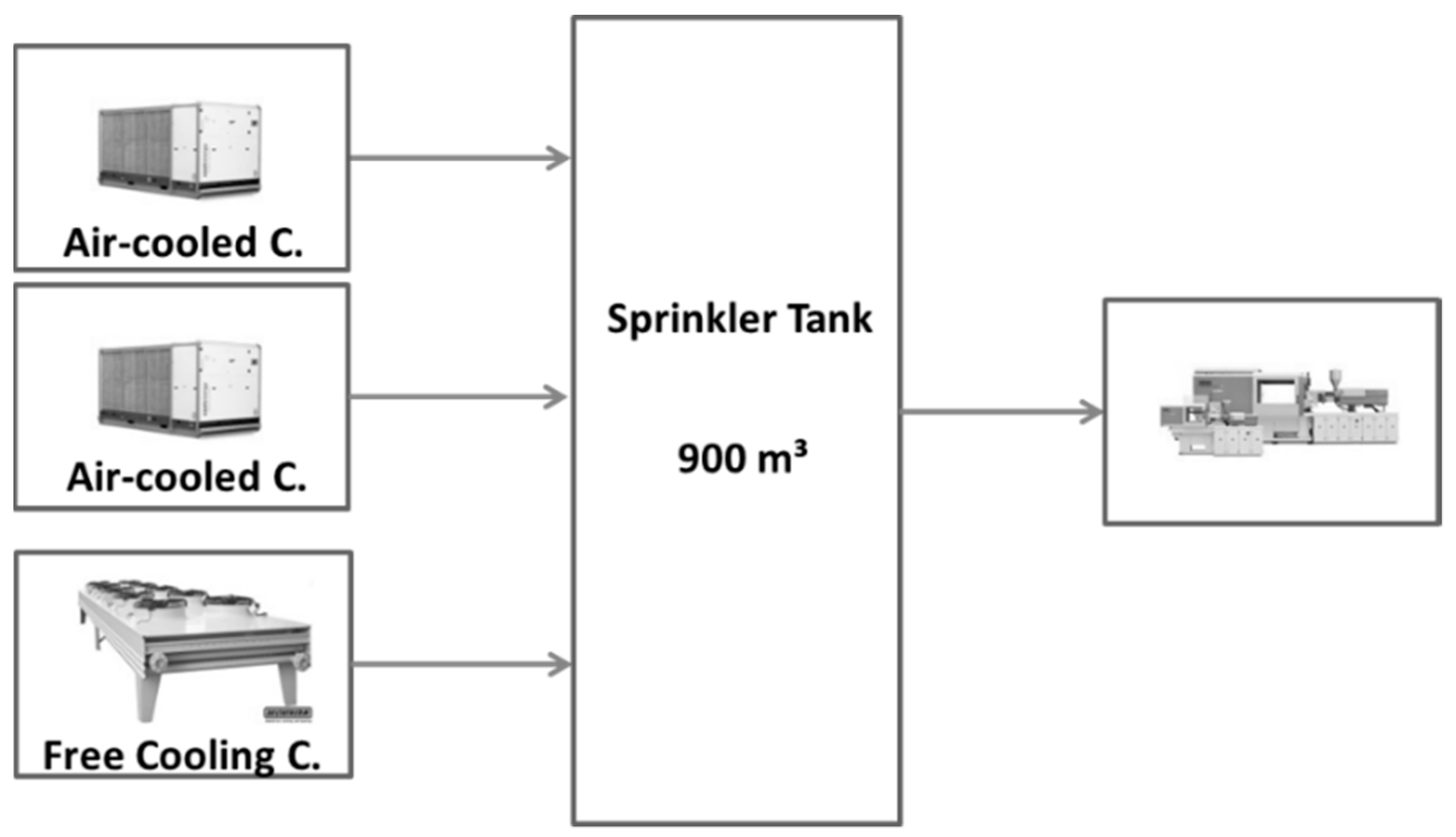
The evaluation of the optimization and the simulation is done by a case study on two plastic processing companies that produce injection-molded parts for the food sector. The purpose of the case study is to establish the level of possible energy cost savings for the considered site. The case study can provide motivation to the site to implement the new optimization approach as well as others to follow a similar procedure. This requires high hygiene standards for the production hall. One is located in Germany and the other in Spain. The variation of the location quantifies the influence of the ambient temperature on the results of the optimization. The injection-molding machines are cooled continuously by two different cooling circuits. The mold-cooling circuit is set at a temperature level of about 14 °C and the machine cooling at about 30 °C. The relatively high process cooling temperature of 14 °C offers the opportunity to integrate free cooling chillers as well as multiple compression chillers. The refrigeration of the molding circuit is carried out by two air-cooled compression chiller machines and a free cooling chiller, which is also used for winter relief. Cooling towers provide the cooling to machine cooling of the plastic processing machines. Moreover, the company has a 900 m³ sprinkler tank that can be used as a cold-water storage tank at a temperature level of 14 °C. The plastic processing companies often have large warehouses. Fire safety regulations require quick access to a high volume of extinguishing water. Because of the multiple operational states, the predictive simulations-based optimization is well-suited for the mold cooling circuit in the plastic processing industry.
In this study, the prediction horizon is varied between 6 and 48 h and the step size is set to 1 h. The NCC is 3 and the NST varies from 4 for the compression chillers to 10 for the free cooling chiller. The cooling demand and the ambient temperature are based on the measured data for the year 2017. For this case study, it is assumed that the forecast for the weather and the cooling demand is perfectly known in each time step. The cooling demand varies between 0 and 190 kW. The simulation time (Tres) is equal to the step size. The maximum cooling energy stored in the cooling tank is fixed by the maximum temperature difference of 3 K and the 900 m³ of water, which results in 3140 kWh. The costs for the optimization are calculated by the product of the current energy consumption of the chillers and the current spot market price for electricity. The prices vary between 75 and 200 €/MWh. The fluctuating price for electricity is also compared to a fixed price scenario. The fixed electricity price is 160 €/MWh. Table 1 gives an overview of the installed cooling utilities and Figure 3 shows the scheme of the cooling system of the plastic processing company.
The following Figure 4 visualizes the partial load performance curve of the air-cooled chiller, according to the Gordon–Ng model, after data processing. The lower the ambient temperature, the higher the EER because of the lower condensing temperature of the chiller and less energy consumed by the fan of the condenser.
4. Results
The results of the predictive simulation-based optimization are compared in five different scenarios. The first scenario is the reference case, which is based on the energy monitoring data of the plastic processing company. In the reference case, the company is located in Kassel, Germany, and has a fixed price for electricity. In the second scenario, the company is also located in Kassel, and the predictive simulation-based optimization is applied to it. To quantify the influence of the prediction horizon, it is varied between 6 and 48 h. To quantify the influence of the ambient temperature on the predictive simulation-based optimization, scenario 3 is identical to scenario 2, except the company’s location is changed from Kassel to Madrid, Spain, and the prediction horizon is set to 48 h. Further, scenario 4 shows the influence of an increased ambient temperature of Kassel by 5 K. Scenario 5 is similar to the second one, except the company purchases its electricity on the EPEX SPOT market and has a variable price. The focus of this scenario is to analyze the influence that a variable electricity price has on the operating schedule of the different chillers. In scenario 6, the company is in Madrid and purchases its electricity from the EPEX SPOT market. Table 2 shows an overview of the different scenarios and the varied parameters of the simulations. The cooling demand for the molding cooling circuit is in all scenarios identically, since hygiene standard forbids any window opening, and therefore the production hall is air-conditioned to a required temperature of 21 °C.
4.1. Prediction Horizon
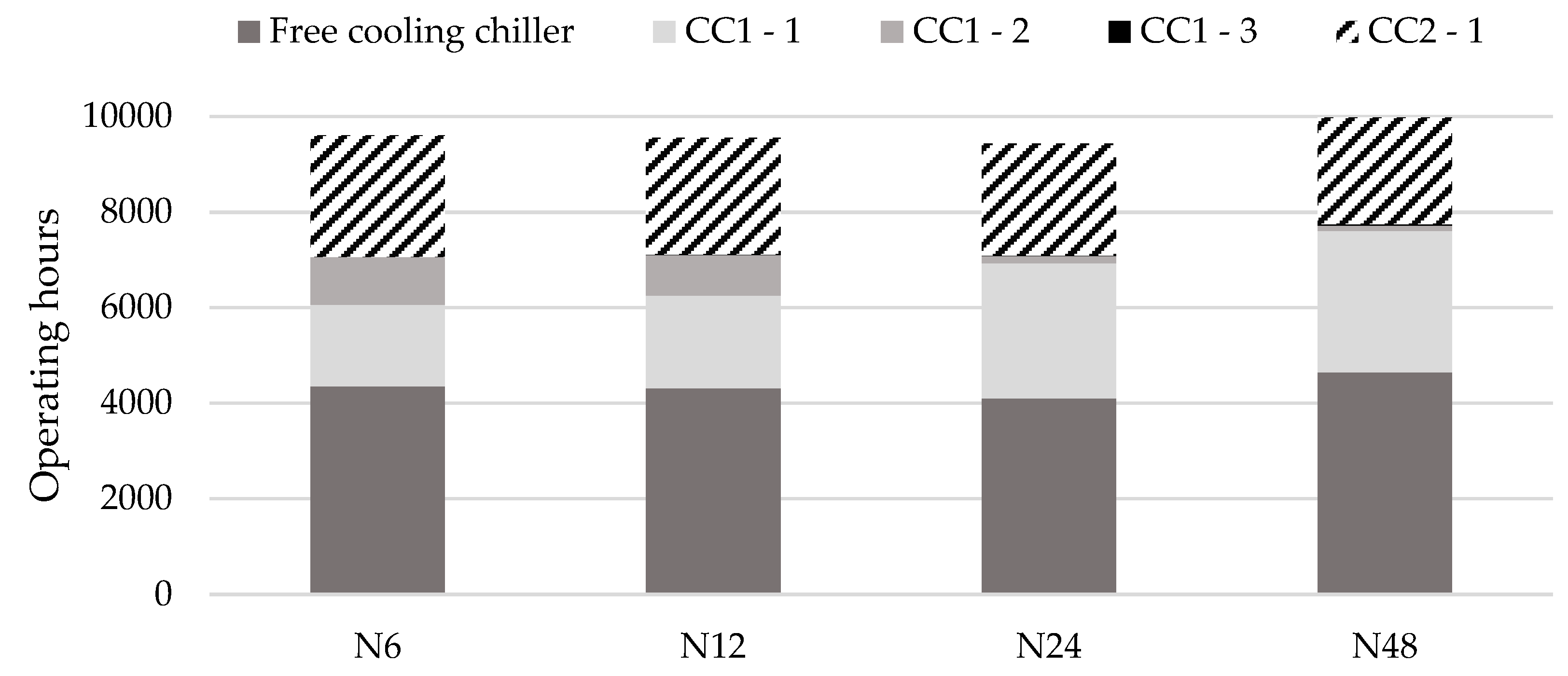
Figure 5 shows the different operating hours of the three chillers for a prediction horizon n between 6 and 48 h. The bottom bar represents the operating hours of the free cooling chiller. The ascending bars show operating hours of the first compression chiller for each stage and the top bar refers to the second compression chiller. Stage 4 of chiller one and stages 2–4 of chiller two are not used in any of the four cases.
It illustrates that the increase in hours of the prediction horizon leads to a rise of the operating hours of the free cooling chiller and increases the operating hours of the two compressions chillers in stage one. The influence on the operating schedule is discernible.
Due to the better efficiency of the free cooling chiller compared to the compression chillers, the electrical energy consumption decreases proportionally to its operating hours. In comparison, the reference case with standard control is also visualized. Figure 6 illustrates the total energy consumption for the four cases, with differing prediction horizons in scenario 2, the reference scenario, as well as the average EER for the year. The results show that the optimization reduces electrical energy consumption by around 38% (N6–N24). A prediction horizon of n = 48 decreases the electrical energy demand by another 5% because of the better charging and discharging strategy of the sprinkler tank.
The difference in energy efficiency and the different operating hours of the free cooling chiller and the stages of the compression chillers result from the charging and discharging strategies based on the different prediction horizons. Figure 7 shows the charge level of the storage tank for the low supply temperature at 14 °C (black line) depending on the time of the year in hours for the four different prediction horizons. The charge level of the high temperature water of 17 °C is the mirror image of it. A prediction horizon of 6 or 12 h results in a minor usage of the energy storage potential of the tank. In the case with a prediction horizon of 24 h, the storage is charged and discharged over 50% of its full capacity in the first and fourth quarter of the year. The full capacity of the storage is used in the case with a prediction horizon of 48 h.
The complete charging and discharging of the tank increase the running hours of the free cooling chillers (Figure 5). With a long prediction horizon, the tank is pre-charged when ambient temperatures fall below 11 °C and discharged in times of high ambient temperatures, minimizing the load on the compression chillers and even placing them in standby mode. This strategy leads to the extra 5% saving potential by extending the prediction horizon to 48 hours.
4.2. Influence of Ambient Temperature
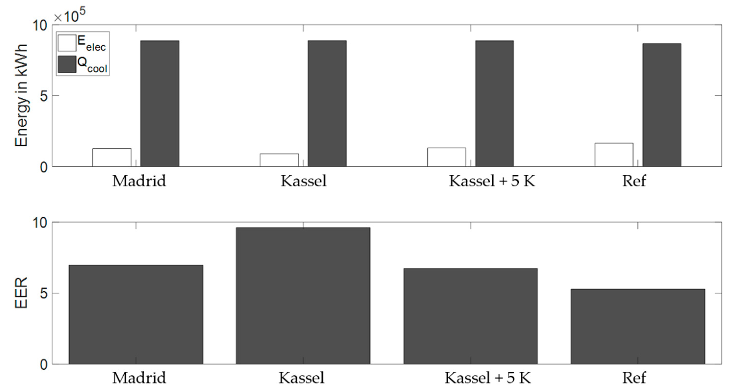
The efficiency of the free cooling chiller and the air-cooled compression chillers depend on the ambient temperature. Lower ambient temperatures allow lower condensing temperatures, resulting in better efficiency. If the ambient temperature is higher than 11 °C, the free cooling chiller does not provide the required cold-water supply temperature. Both effects have an influence on the energy-saving potential of the predictive simulation-based optimization. Hence, in scenario 3, the plastic processing company is moved to Madrid, Spain, to have a different ambient temperature profile. In scenario 4, the German temperature profile is lifted by 5 K. Figure 8 shows the total energy consumption and EER for one year in comparison to the reference case and scenario 2. All optimizations are based on a prediction horizon of 48 h, since the previous analyses in Section 4.1 conclude that this is the best horizon to maximize energy savings.
The change in the ambient temperature reduces the energy-saving potential for Madrid to 23% and, for scenario 4, to 19% compared to the reference case. Because of reduced running hours of the free cooling chiller in scenarios 3 and 4, the energy efficiency is significantly lower compared to scenario 2. However, the analysis of the different ambient temperatures also shows that the predictive simulation-based optimization together with the sprinkler tank reduces the electrical energy consumption in warmer regions. Although the energy-saving potential is reduced for warmer ambient temperatures, there is still a significant reduction compared to the reference case.
4.3. Variable Electricity Prices
In the previous scenarios, the electricity price for the plastic processing company is fixed to 16 euro cent/kWh. In scenarios 5 and 6, the electricity procurement is via the day-ahead exchange market in Germany. All taxes, costs, and the German renewable energy levy are included in the model. To benefit from purchasing electricity with a variable price, it is required to shift loads. The sprinkler tank enables the cold utility system to store cold-water in times of little or no demand. This allows the optimization algorithm to start chillers in times of low electricity prices and stop the machines in times of high prices. This increases the optimization options. Figure 9 shows the results of the simulation for the variable cost option in comparison to the fixed price and the reference case. On the left y axis, the thermal and electrical energy consumptions are visualized, and the costs are shown on the right y axis.
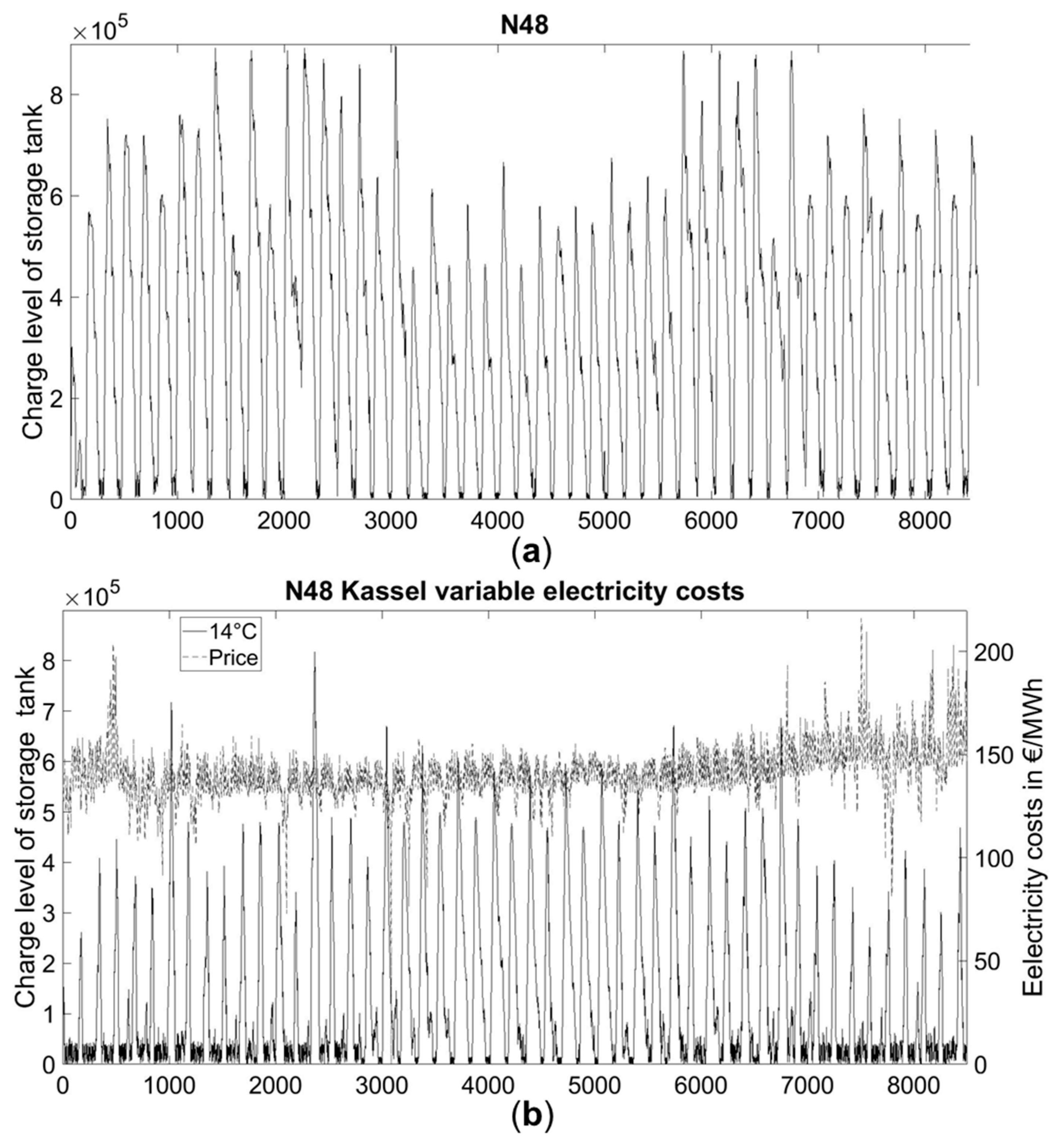
Under scenarios 5 and 6, the electrical energy consumption for Kassel increases by 7% and, for Madrid, by 0.4%, but the total energy costs for the cooling systems are reduced. For the plastic processing company in Kassel, the electricity procurement via the spot market reduces the costs by around 9.3%. For the site in Madrid, the costs reduction is about 12%. The increased electrical energy consumption is due to the reduction of the operating hours of the free cooler and the simultaneous increase in the use of the compression chiller. This leads to a decreased overall efficiency of the system. However, the lower efficiency is compensated by the lower prices for the electrical energy on the spot market in comparison to a fixed electricity price. Figure 10 shows the comparison of the charge level of the sprinkler tanks for fixed and variable price scenarios.
In Figure 10b, the electricity price is shown on the right y axis. In comparison to the fixed price scenario, the storage tank is never fully charged in the variable price scenario. Although both prediction horizons are equal, the results of the optimization differ for minimizing the costs. The different charging and discharging strategies are the reason for different electrical energy consumption and the different total energy costs.
4.4. Results Summary
Table 3 summarizes the results for the comparison of the different prediction horizons, the influence of the ambient temperature, and the effect of purchasing electricity for a variable price. The savings in percentage for energy and costs use the basis of the reference case.
5. Conclusions and Outlook
The study developed a predictive simulation-based optimization of a cooling system with continuous self-learning performance curve models that saves electrical energy by optimal charging and discharging of the sprinkler tank. The optimization reduced electrical energy costs via electricity procurement on the EPEX SPOT market. Results for the case study concluded that the control strategy of the optimization together with the installation of cold-water storage tanks with a significant volume and a free cooling chiller could save over 43% of the electrical energy in comparison to the reference case. To utilize the full potential of the storage tank, a prediction horizon of 48 h was necessary. In comparison, a prediction horizon of 6 h saved up to 38% of electricity use. The difference in the prediction horizon had minimal impact on the computation time. A longer prediction horizon increased the energy savings, but the available thermal storage capacity limits it. In further analyses, the influence of the modeling error and weather forecast changes on the optimal operational strategies as well as the potential for exergy and entropy considerations may be investigated.
The study further investigated the effects of ambient temperature due to different plant locations as well as a variable electricity spot price. The ambient temperature profile had a significant influence on the energy-saving potential. The higher the average ambient temperature, the lower the energy saving—however, the optimization strategy still saved around 20% in warmer regions. Electricity procurement via the EPEX SPOT market led to a slight increase in electrical energy consumption but saved 9.3% to 12% of the energy costs. For the analyzed plastic processing company, the differences in the electricity price were low but still influenced the cooling utility system. If the company should economically support the electricity grid, the price differences need to be higher or include extra incentives. For example, a dynamic tax on electricity based on the instantaneous share of renewable electricity generation presents a chance to increase the differences in the variable prices and make demand-side management more attractive for medium-sized companies.
Author Contributions
Responsible for the conceptualization, R.-H.P. and F.S.; methodology, R.-H.P. and H.M.; validation, R.-H.P.; investigation, R.-H.P. and H.D.; data curation, H.D.; writing—original draft preparation, R.-H.P.; writing—review and editing, F.S., H.M. and T.G.W.; visualization, R.-H.P.; supervision, T.G.W.; funding acquisition, R.-H.P.
Funding
This research received no external funding.
Acknowledgments
The authors gratefully acknowledge the financial support of the Rud. Otto-Meyer-Umwelt-Stiftung and the support of the EU project “Sustainable Process Integration Laboratory – SPIL”, project No. CZ.02.1.01/0.0/0.0/15_003/0000456 funded by EU “CZ Operational Programme Research and Development, Education”, Priority 1: Strengthening capacity for quality research.
Conflicts of Interest
The authors declare no conflict of interest.
Nomenclature
| Ax | Regression coefficients for Gordon–Ng model |
| Bx | Regression coefficients for free cooling chiller |
| CC | Cooling capacity |
| Specific heat capacity of water | |
| E | Energy |
| EER | Energy efficiency ratio |
| FC | Free cooling chiller |
| Enthalpy flow | |
| MPC | Model predictive control |
| Mass of water in storage tank | |
| Mass of water in storage tank at cold water temperature of chiller | |
| Mass of water in storage tank at cold water return temperature of chiller | |
| NCC | Number of chilling machines |
| NT | Timesteps |
| NST | Maximum states of chilling machine |
| PLR | Part-load ratio |
| Pel, CC | Electric power of chiller |
| cool | Cooling load |
| vertical | Vertical heat conduction |
| losses | Heat input by storage wall |
| Qminus | Current cooling energy of sprinkler tank |
| Qpred | Total cooling demand for all timesteps |
| Qplus | Current cooling capacity of sprinkler tank |
| Rad | Heat input by radiation |
| SC | Starting costs |
| St | Operating state of chilling machine |
| Tamb | Ambient temperature |
| Tcond | Condensing temperature of chiller |
| Tcold | Cold water temperature of chiller |
| TRes | Simulation time |
| TSt | Storage temperature |
| U | Internal energy |
| Xtnst | State of chilling machine |
| Ztn | On/off Variable |
References
- Heinrich, C.; Witti, S.; Albring, P.; Richter, L.; Safarik, M.; Böhm, U.; Hantsch, A. Nachhaltige Kälteversorgung in Deutschland an den Beispielen Gebäudeklimatisierung und Industrie. 2014. Available online: https://www.umweltbundesamt.de/sites/default/files/medien/378/publikationen/climate_change_25_2014_nachhaltige_kaelteversorgung_in_deutschland_1.pdf (accessed on 2 May 2018).
- Peesel, R.-H.; Schlosser, F.; Schaumburg, C.; Meschede, H. Prädiktive simulationsgestützte Optimierung von Kältemaschinen im Verbund. In Simulation in Produktion und Logistik 2017; Wenzel, S., Peter, T., Eds.; Kassel University Press: Kassel, Germany, 2017; pp. 69–78. ISBN 978-3-7376-0192-4. [Google Scholar]
- Clausen, U.; Diekmann, D.; Baudach, J.; Pöting, M. Mathematical Optimisation and Simulation of Parcel Transshipment Terminals—Better Solutions by Linking These Two Complementary Methods. Simul. Prod. Logist. 2015, 2015, 279–288. [Google Scholar]
- Augenstein, E. Betriebsoptimierung von Kältezentralen—Einsparpotentiale durch situationsabhängige Einsatzregeln. KKA Kälte Klima Aktuell Sonderausgabe Großkältetechnik. 2009. Available online: http://www.perpendo.de/files/kka-2009.pdf (accessed on 17 May 2019).
- Ahn, B.C.; Mitchell, J.W. Optimal control development for chilled water plants using a quadratic representation. Energy Build. 2001, 33, 371–378. [Google Scholar] [CrossRef]
- Mu, B.; Li, Y.; House, J.M.; Salsbury, T.I. Real-time optimization of a chilled water plant with parallel chillers based on extremum seeking control. Appl. Energy 2017, 208, 766–781. [Google Scholar] [CrossRef]
- Hovgaard, T.G.; Edlund, K.; Jorgensen, J.B. The potential of Economic MPC for power management. In Proceedings of the 49th IEEE Conference on Decision and Control (CDC), Atlanta, GA, USA, 15–17 December 2010; pp. 7533–7538. [Google Scholar]
- Braun, J.E. Methodologies for the Design and Control of Central Cooling Plants. Ph.D. Thesis, University of Wisconsin, Madison, WI, USA, 1988. [Google Scholar]
- Olson, R.T.; Liebman, J.S. Optimization of a chilled water plant using sequential quadratic programming. Eng. Optim. 1990, 15, 171–191. [Google Scholar] [CrossRef]
- Chang, Y.-C.; Lin, F.-A.; Lin, C.H. Optimal chiller sequencing by branch and bound method for saving energy. Energy Convers. Manag. 2005, 46, 2158–2172. [Google Scholar] [CrossRef]
- Chang, Y.-C. An Outstanding Method for Saving Energy—Optimal Chiller Operation. IEEE Trans. Energy Convers. 2006, 21, 527–532. [Google Scholar] [CrossRef]
- Chang, Y.-C.; Chan, T.-S.; Lee, W.-S. Economic dispatch of chiller plant by gradient method for saving energy. Appl. Energy 2010, 87, 1096–1101. [Google Scholar] [CrossRef]
- Chang, Y.-C. Genetic algorithm based optimal chiller loading for energy conservation. Appl. Therm. Eng. 2005, 25, 2800–2815. [Google Scholar] [CrossRef]
- Chang, Y.-C.; Chen, W.-H.; Lee, C.-Y.; Huang, C.-N. Simulated annealing based optimal chiller loading for saving energy. Energy Convers. Manag. 2006, 47, 2044–2058. [Google Scholar] [CrossRef]
- Lee, W.-S.; Lin, L.-C. Optimal chiller loading by particle swarm algorithm for reducing energy consumption. Appl. Therm. Eng. 2009, 29, 1730–1734. [Google Scholar] [CrossRef]
- Powell, K.M.; Cole, W.J.; Ekarika, U.F.; Edgar, T.F. Optimal chiller loading in a district cooling system with thermal energy storage. Energy 2013, 50, 445–453. [Google Scholar] [CrossRef]
- Huang, S.; Zuo, W.; Sohn, M.D. A New Method for The Optimal Chiller Sequencing Control. In Proceedings of the 14th Conference of IBPSA, Hyderabad, India, 7–9 December 2015; pp. 316–323. [Google Scholar]
- Thangavelu, S.R.; Myat, A.; Khambadkone, A. Energy optimization methodology of multi-chiller plant in commercial buildings. Energy 2017, 123, 64–76. [Google Scholar] [CrossRef]
- Kapoor, K.; Powell, K.; Cole, W.; Kim, J.; Edgar, T. Improved Large-Scale Process Cooling Operation through Energy Optimization. Processes 2013, 1, 312–329. [Google Scholar] [CrossRef]
- Cole, W.J.; Powell, K.M.; Edgar, T.F. Optimization and advanced control of thermal energy storage systems. Rev. Chem. Eng. 2012, 28, 81–99. [Google Scholar] [CrossRef]
- Kircher, K.J.; Zhang, K.M. Model predictive control of thermal storage for demand response. In Proceedings of the American Control Conference (ACC), Chicago, IL, USA, 1–3 July 2015. [Google Scholar]
- Ma, Y.; Borrelli, F.; Hencey, B.; Coffey, B.; Bengea, S.; Haves, P. Model Predictive Control for the Operation of Building Cooling Systems. IEEE Trans. Contr. Syst. Technol. 2012, 20, 796–803. [Google Scholar] [CrossRef] [Green Version]
- Soler, M.S.; Sabaté, C.C.; Santiago, V.B.; Jabbari, F. Optimizing performance of a bank of chillers with thermal energy storage. Appl. Energy 2016, 172, 275–285. [Google Scholar] [CrossRef]
- Peesel, R.-H.; Schlosser, F.; Schaumburg, C.; Meschede, H.; Dunkelberg, H.; Walmsley, T.G. Predictive Simulation-based Optimisation of Cooling System Including a Sprinkler Tank. Chem. Eng. Trans. 2018, 2018, 349–354. [Google Scholar]
- Vaghefi, A.; Jafari, M.A.; Bisse, E.; Lu, Y.; Brouwer, J. Modeling and forecasting of cooling and electricity load demand. Appl. Energy 2014, 136, 186–196. [Google Scholar] [CrossRef] [Green Version]
- Kwok, S.S.K.; Yuen, R.K.K.; Lee, E.W.M. An intelligent approach to assessing the effect of building occupancy on building cooling load prediction. Build. Environ. 2011, 46, 1681–1690. [Google Scholar] [CrossRef]
- Li, Q.; Meng, Q.; Cai, J.; Yoshino, H.; Mochida, A. Predicting hourly cooling load in the building: A comparison of support vector machine and different artificial neural networks. Energy Convers. Manag. 2009, 50, 90–96. [Google Scholar] [CrossRef]
- Gordon, J.M.; Ng, K.C. Cool Thermodynamics. The Engineering and Physics of Predictive, Diagnostic and Optimization Methods for Cooling Systems; Cambridge International Science: Cambridge, UK, 2001; ISBN 1898326908. [Google Scholar]
- Brenner, A.; Kausch, C.; Kirschbaum, S.; Lepple, H.; Zens, M. Effizienzsteigerung in Einem komplexen Kühlwassersystem. Einsatz von Simulationswerkzeugen. 2014. Available online: http://www.perpendo.de/files/kka-2014.pdf (accessed on 21 October 2016).
- Lee, T.-S.; Liao, K.-Y.; Lu, W.-C. Evaluation of the suitability of empirically-based models for predicting energy performance of centrifugal water chillers with variable chilled water flow. Appl. Energy 2012, 93, 583–595. [Google Scholar] [CrossRef]
- Gurobi Optimization, L.L.C. Gurobi Optimizer Reference Manual. 2018. Available online: http://www.gurobi.com/documentation/8.1/ (accessed on 17 May 2019).
- Wemhöner, C.; Hafner, B.; Schwarzer, K. Simulation of Solar Thermal Systemswith Carnot Blockset in the Environment Matlab Simulink. 2000. Available online: http://ptp.irb.hr/upload/mape/kuca/11_Carsten_Wemhoener_SIMULATION_OF_SOLAR_THERMAL_SYSTEMS_WITH.pdf (accessed on 14 June 2016).
Figure 1.
Simulation-based optimization scheme.

Figure 2.
(a) Data overview before and after data pre-processing for the electrical load of chiller 1; (b) data overview before and after data pre-processing for the thermal load of chiller 1.
Figure 2.
(a) Data overview before and after data pre-processing for the electrical load of chiller 1; (b) data overview before and after data pre-processing for the thermal load of chiller 1.

Figure 3.
Scheme of cooling system plastic processing company.

Figure 4.
Part-load performance curve for air-cooled compression chiller.

Figure 5.
Operating hours of chillers in different stages for varying prediction horizons.

Figure 6.
Energy savings and energy efficiency ratio (EER) comparison for varying prediction horizons.
Figure 6.
Energy savings and energy efficiency ratio (EER) comparison for varying prediction horizons.

Figure 7.
Charge level of the storage tank for varying prediction horizons.

Figure 8.
Energy savings and EER comparison for different ambient temperatures.

Figure 9.
Comparison of variable and fixed price optimization.

Figure 10.
(a) Charge level of storage tank for a fixed electricity price; (b) charge level of storage tank for variable price scenarios.
Figure 10.
(a) Charge level of storage tank for a fixed electricity price; (b) charge level of storage tank for variable price scenarios.


Table 1.
Utility system of the plastic processing company.
| Utility | Quantity | Temperature Level | Cooling Capacity | Number of Stages | Lower Bound | Step Size |
|---|---|---|---|---|---|---|
| Air-cooled scroll chiller | 2 | 14 °C | 200 kW | 4 | 25% | 25% |
| Free cooling chiller | 1 | 14 °C | 200 kW | 10 | 10% | 10% |
| Cooling towers | 2 | 30 °C | 250 kW | 4 | 25% | 25% |
| Sprinkler tank | 1 | 14 °C | 3140 kWh | - | - | - |
Table 2.
Overview of simulated scenarios and parameters.
| Scenario | Location | Prediction Horizon (h) | Electricity Price | Optimization |
|---|---|---|---|---|
| 1. Reference case | Kassel | None | Fixed 16 ct/kWh | No |
| 2. Prediction horizon | Kassel | 6–48 | Fixed 16 ct/kWh | Yes |
| 3. Ambient temperature | Madrid | 48 | Fixed 16 ct/kWh | Yes |
| 4.Ambient temperature + 5 | Kassel + 5 K | 48 | Fixed 16 ct/kWh | Yes |
| 5. Flexible electricity price | Kassel | 48 | EPEX SPOT market | Yes |
| 6. Ambient temperature and flexible electricity price | Madrid | 48 | EPEX SPOT market | Yes |
Table 3.
Overview of optimization results.
| Scenario | Electrical Energy in kWh | Energy Savings in % | Energy Costs in € | Cost Savings in % |
|---|---|---|---|---|
| 1. Reference case | 164,062 | 0 | 26,250 | 0 |
| 2.1 Prediction horizon N6 | 101,760 | 38.0 | 16,282 | 38.0 |
| 2.2 Prediction horizon N12 | 101,540 | 38.1 | 16,245 | 38.1 |
| 2.3 Prediction horizon N24 | 99,485 | 39.4 | 15,918 | 39.4 |
| 2.4 Prediction horizon N48 | 92,248 | 43.7 | 14,760 | 43.8 |
| 3. Ambient temperature | 127,270 | 22.4 | 20,363 | 22.4 |
| 4.Ambient temperature + 5 | 131,740 | 19.7 | 21,078 | 19.7 |
| 5. Flexible electricity price | 98,697 | 39.8 | 13,727 | 47.7 |
| 6. Ambient temperature and flexible electricity price | 127,775 | 22.1 | 17,910 | 31.8 |
© 2019 by the authors. Licensee MDPI, Basel, Switzerland. This article is an open access article distributed under the terms and conditions of the Creative Commons Attribution (CC BY) license (http://creativecommons.org/licenses/by/4.0/).
Share and Cite
MDPI and ACS Style
Peesel, R.-H.; Schlosser, F.; Meschede, H.; Dunkelberg, H.; Walmsley, T.G. Optimization of Cooling Utility System with Continuous Self-Learning Performance Models. Energies 2019, 12, 1926. https://doi.org/10.3390/en12101926
AMA Style
Peesel R-H, Schlosser F, Meschede H, Dunkelberg H, Walmsley TG. Optimization of Cooling Utility System with Continuous Self-Learning Performance Models. Energies. 2019; 12(10):1926. https://doi.org/10.3390/en12101926
Chicago/Turabian StylePeesel, Ron-Hendrik, Florian Schlosser, Henning Meschede, Heiko Dunkelberg, and Timothy G. Walmsley. 2019. "Optimization of Cooling Utility System with Continuous Self-Learning Performance Models" Energies 12, no. 10: 1926. https://doi.org/10.3390/en12101926
Note that from the first issue of 2016, this journal uses article numbers instead of page numbers. See further details here.