Energy Management through Cost Forecasting for Residential Buildings in New Zealand


Abstract
1. Introduction
2. Literature Review
2.1. Influencing Factors of Residential Energy Use
2.2. Cost Forecasting Methods
2.3. Energy Consumption Forecasting
3. Research Methods
3.1. Data
3.2. Correlation Analysis
3.3. Exponential Smoothing
3.3.1. Holt-Winters Method
3.3.2. Multiplicative Holt-Winters Method
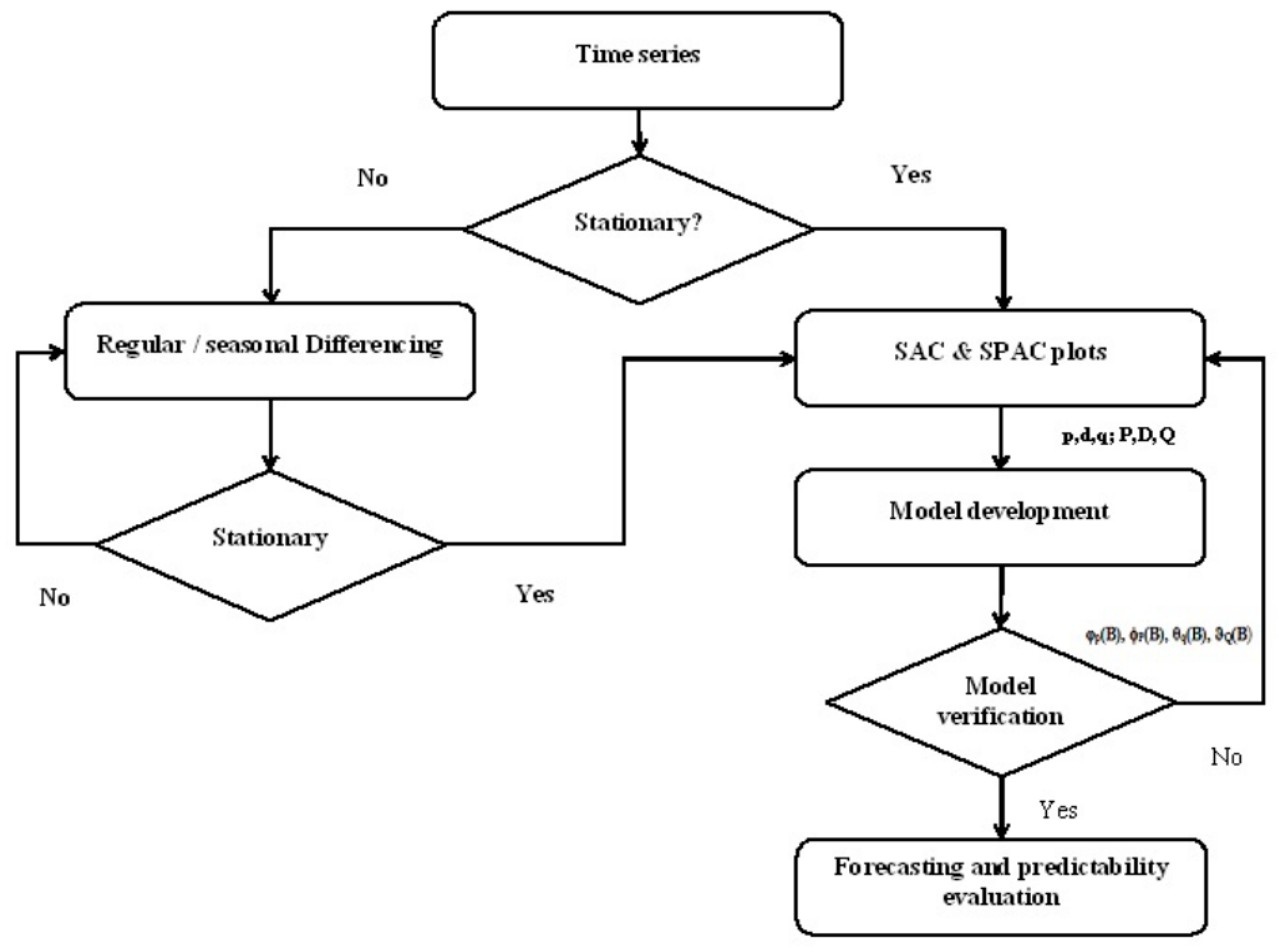
3.4. Autoregressive Integrated Moving Average (ARIMA)
3.5. Error Measure for Model Comparison
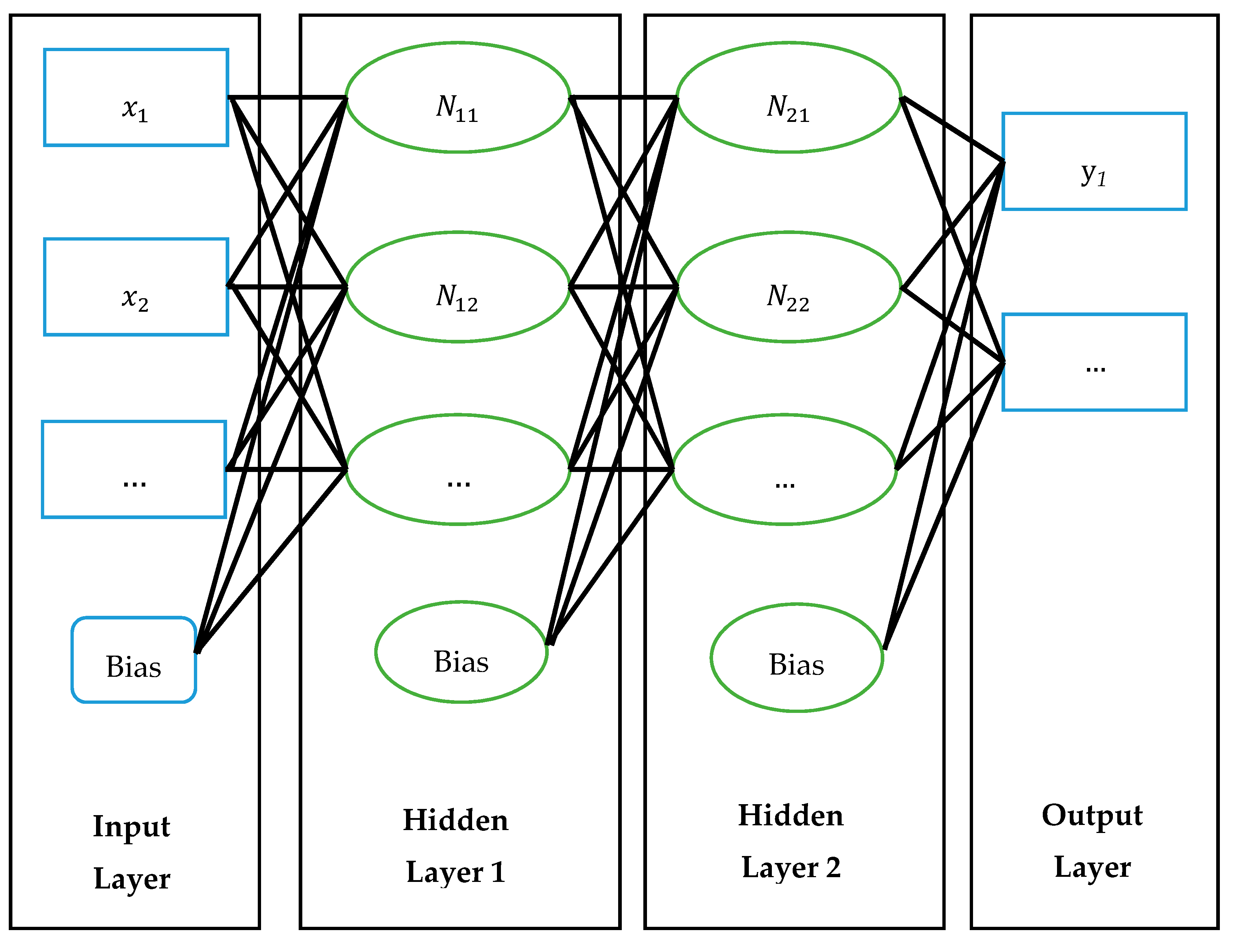
3.6. Multilayer Artificial Neutral Networks
3.7. t-Test
4. Data Analysis
4.1. Correlation Analysis Results
4.2. Exponential Models for Building Cost
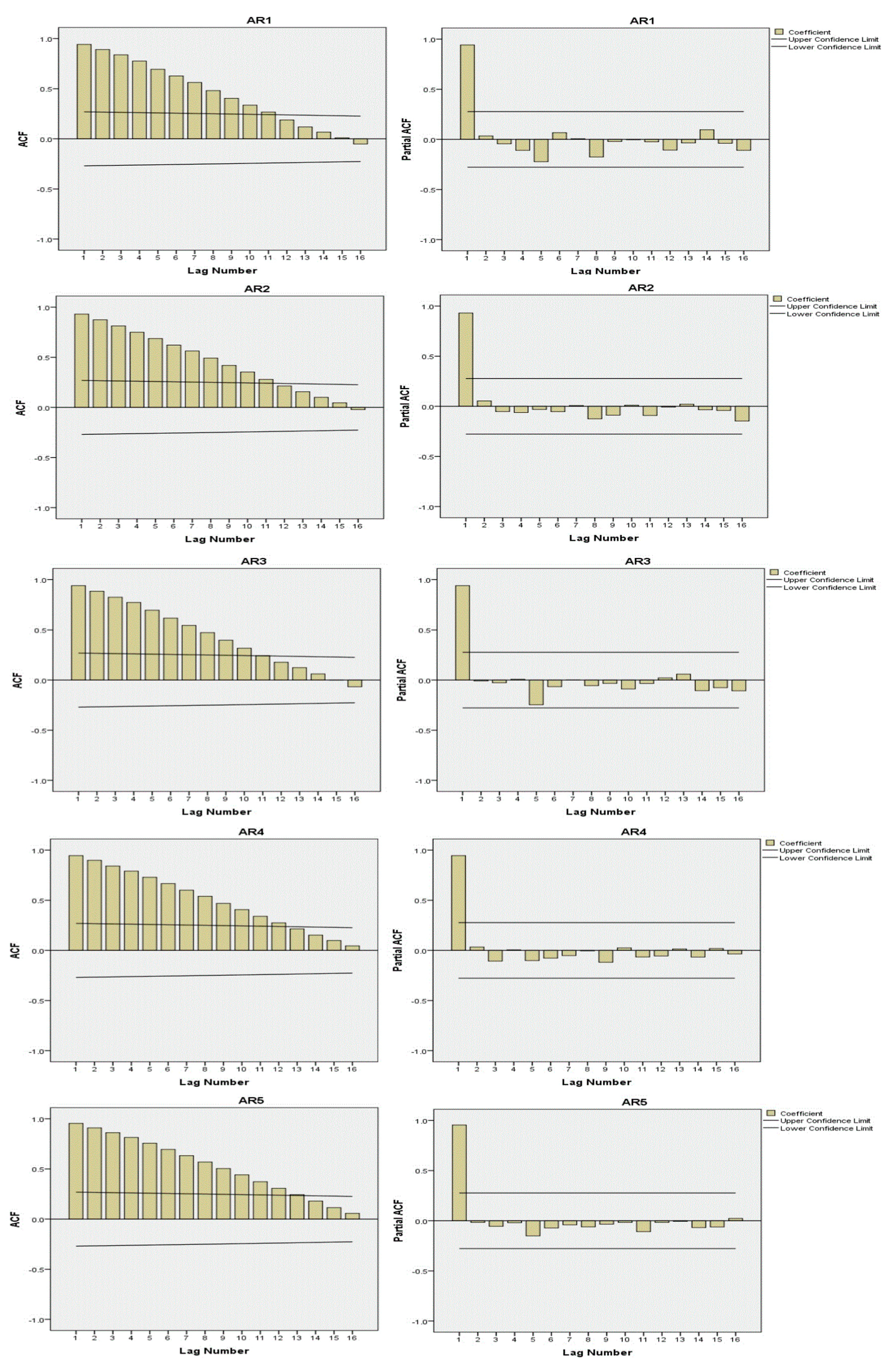
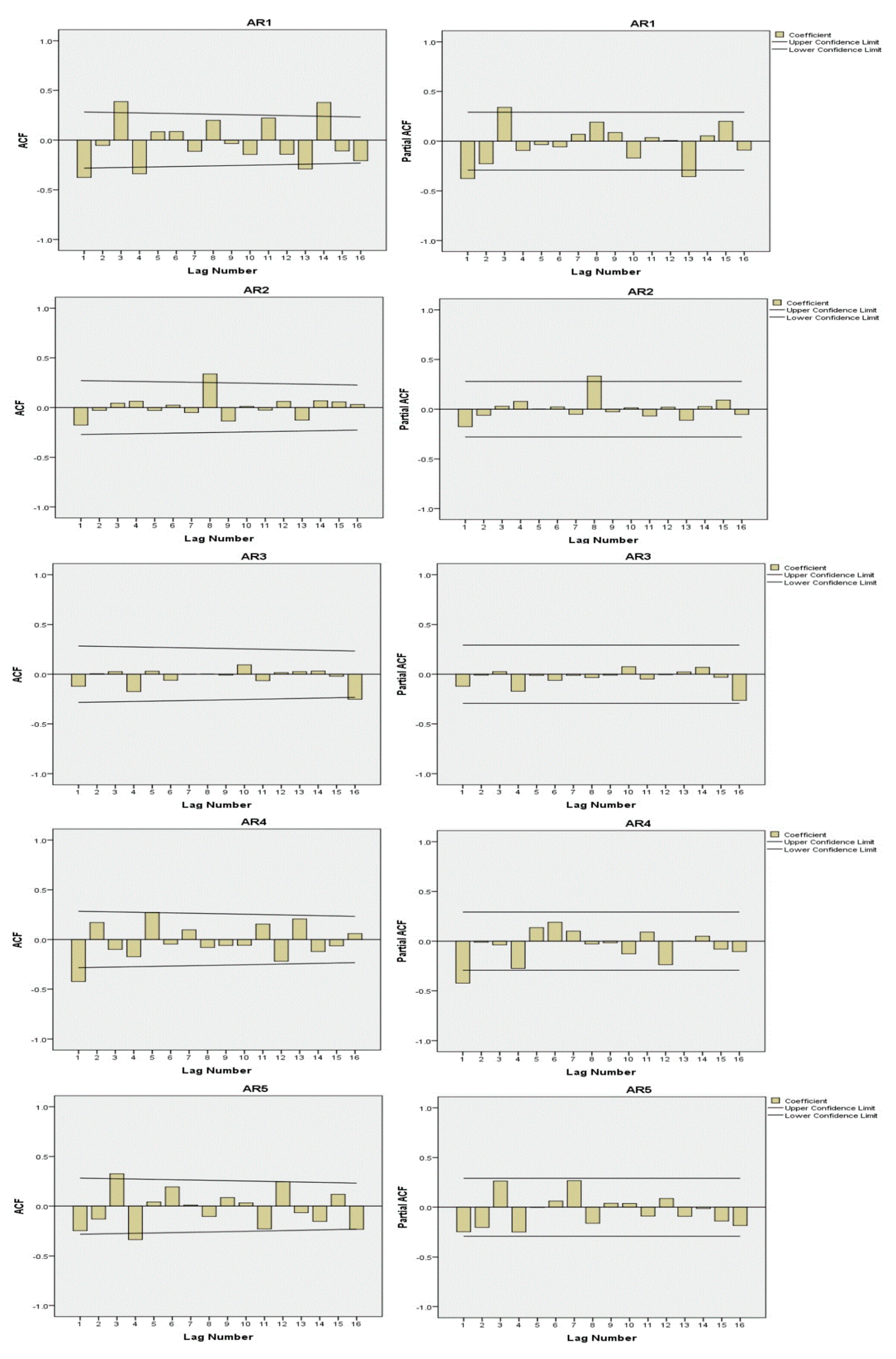
4.3. Seasonal ARIMA Models
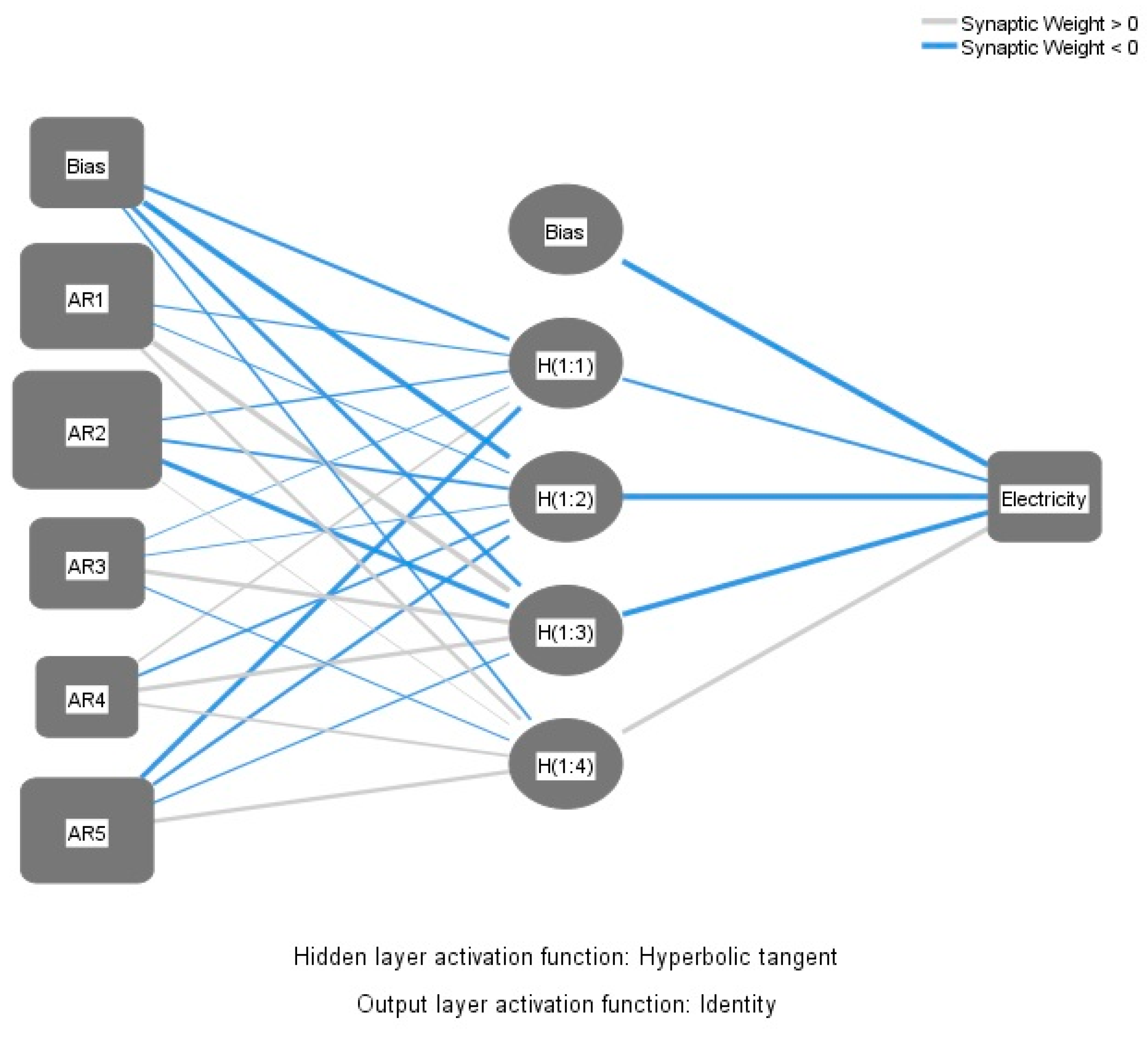
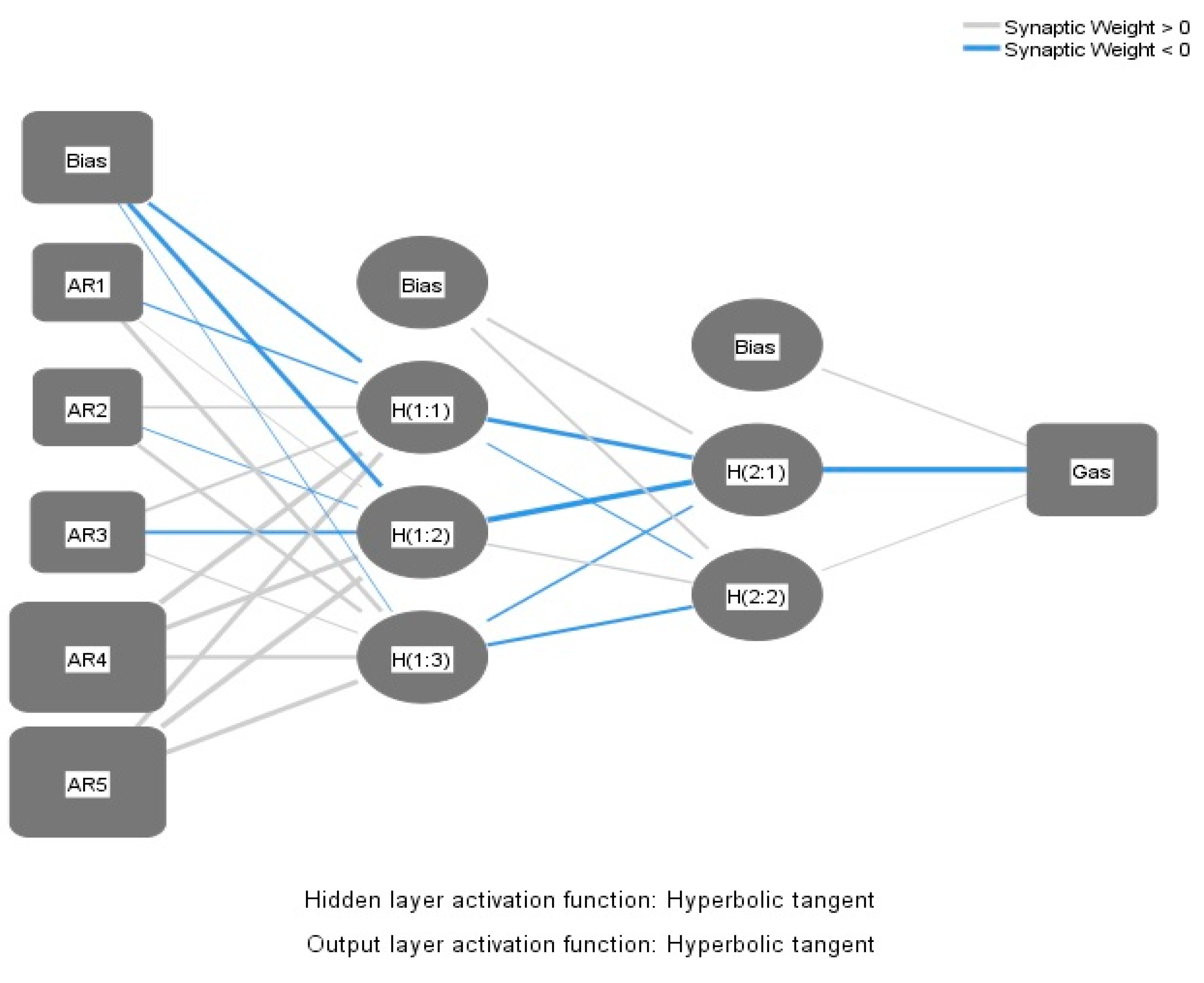
4.4. ANN Models
5. Results Discussion
6. Conclusions
Author Contributions
Funding
Acknowledgments
Conflicts of Interest
Abbreviations
| ACF | Auto-Correlation Function |
| ANNs | Artificial Neutral Networks |
| AR | Autoregressive |
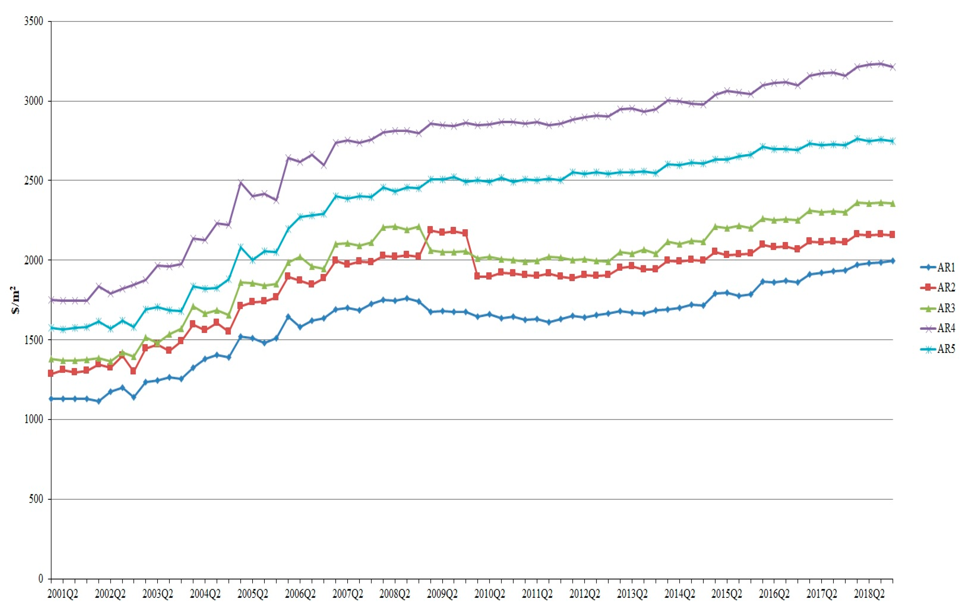
| AR1 | One-storey House |
| AR2 | Two-storey House |
| AR3 | Townhouse |
| AR4 | Apartment |
| AR5 | Retirement Village |
| ARIMA | Autoregressive Integrated Moving Average |
| BIC | Bayesian Information Criterion |
| ES | Exponential Smoothing Method |
| HVAC | Heating, Ventilation and Air Conditioning |
| HW | Holt-Winter Method |
| MA | Moving Average |
| MAE | Mean Absolute Error |
| MAPE | Mean Absolute Percentage Error |
| MHW | Multiplicative Holt-Winter Method |
| PACF | Partial Auto-Correlation Function |
| RMSE | Root Mean Square Error |
| SAC | Sample Auto-Correlation Function |
| SAR | Seasonal Autoregressive |
| SE | Standard Error |
| SSE | Sum of Squared Error |
| SMA | Seasonal Moving Average |
| SPAC | Sample Partial Auto-Correlation Function |
References
- Isaacs, N.; Camilleri, M.; French, L.; Pollard, A.; Saville-Smith, K.; Fraser, R.; Rossouw, P.; Jowett, J. Energy Use in New Zealand Households Report on the Year 10 Analysis for the Household Energy End-Use Project; Building Research Association of New Zealand (BRANZ): Porirua, New Zealand, 2016; pp. 1–134. [Google Scholar]
- RBNZ. Housing Risks Require a Broad Policy Response; Reserve Bank of New Zealand: Wellington, New Zealand, 2016. [Google Scholar]
- Holt, C.C. Forecasting seasonals and trends by exponentially weighted moving averages. Int. J. Forecast. 2004, 1, 5–10. [Google Scholar] [CrossRef]
- Brown, R.G. Statistical Forecasting for Inventory Control; McGraw-Hill: New York, NY, USA, 1959. [Google Scholar]
- Hyndman, R.J.; Koehler, A.B.; Ord, J.K.; Snyder, R.D. Forecasting with Exponential Smoothing: The State Space Approaches; Springer-Verlag: Berlin, Germany, 2008. [Google Scholar]
- Box, G.E.P.; Jenkins, G.M.; Reinsel, G.C. Time Series Analysis: Forecasting and Control; Holden-Day: Oakland, CA, USA, 2011. [Google Scholar]
- Gujarati, D.N. Basic Econometrics; Elsevier: Rio de Janeiro, Brasil, 2006. [Google Scholar]
- Ahmad, A.S.; Hassan, M.Y.; Abdullah, M.P.; Rahman, H.A.; Hussin, F.; Abdullah, H.; Saidur, R. A review on applications of ANN and SVM for building electrical energy consumption forecasting. Renew. Sustain. Energy Rev. 2014, 33, 102–109. [Google Scholar] [CrossRef]
- Bhandari, M.; Shrestha, S.; New, J. Evaluation of weather datasets for building energy simulation. Energy Build. 2012, 49, 109–118. [Google Scholar] [CrossRef]
- Hopfe, C.J.; Hensen, J.L.M. Uncertainty analysis in building performance simulation for design support. Energy Build. 2011, 43, 2798–2805. [Google Scholar] [CrossRef]
- Kaynakli, O. A review of the economical and optimum thermal insulation thickness for building applications. Renew. Sustain. Energy Rev. 2012, 16, 415–425. [Google Scholar] [CrossRef]
- Byun, J.; Shin, T. Design and implementation of an energy-saving lighting control system considering user satisfaction. IEEE Trans. Consum. Electron. 2018, 64, 61–68. [Google Scholar] [CrossRef]
- Yu, Z.; Fung, B.C.M.; Haghighat, F.; Yoshino, H.; Morofsky, E. A systematic procedure to study the influence of occupant behavior on building energy consumption. Energy Build. 2010, 43, 1409–1417. [Google Scholar] [CrossRef]
- Gill, Z.M.; Tierney, M.J.; Pegg, I.M.; Allan, N. Low energy dwellings: The contribution of behaviours to actual performance. Build. Res. Inf. 2010, 38, 491–508. [Google Scholar] [CrossRef]
- Bichiou, Y.; Krarti, M. Optimization of envelope and HVAC systems selection for residential buildings. Energy Build. 2011, 43, 3373–3382. [Google Scholar] [CrossRef]
- Tuhus-Dubrow, D.; Krarti, M. Genetic-algorithm based approach to optimize building envelope design for residential buildings. Build. Environ. 2010, 45, 1574–1581. [Google Scholar] [CrossRef]
- Gasparella, A.; Pernigotto, G.; Cappelletti, F.; Romagnoni, P.; Baggio, P. Analysis and modelling of window and glazing systems energy performance for a well insulated residential building. Energy Build. 2011, 43, 1030–1037. [Google Scholar] [CrossRef]
- Ihm, P.; Krarti, M. Design optimization of energy efficient residential buildings in Tunisia. Build. Environ. 2012, 58, 81–90. [Google Scholar] [CrossRef]
- Jaber, S.; Ajib, S. Optimum, technical and energy efficiency design of residential building in Mediterranean region. Energy Build. 2011, 43, 1829–1834. [Google Scholar] [CrossRef]
- Kapsalaki, M.; Leal, V.; Santamouris, M. A methodology for economic efficient design of net zero energy buildings. Energy Build. 2012, 55, 765–778. [Google Scholar] [CrossRef]
- Yao, J. Energy optimization of building design for different housing units in apartment buildings. Appl. Energy 2012, 94, 330–337. [Google Scholar] [CrossRef]
- Magnier, L.; Haghighat, F. Multi objective optimization of building design using TRNSYS simulations, geneticalgorithm, and artificial neural network. Build. Environ. 2010, 45, 739–746. [Google Scholar] [CrossRef]
- Domínguez, S.; Sendra, J.J.; León, A.L.; Esquivias, P.M. Towards energy demand reduction in social housing buildings: Envelope system optimization strategies. Energies 2012, 5, 2263–2287. [Google Scholar] [CrossRef]
- Griego, D.; Krarti, M.; Hernández-Guerrero, A. Optimization of energy efficiency and thermal comfort measures for residential buildings in Salamanca, Mexico. Energy Build. 2012, 54, 540–549. [Google Scholar] [CrossRef]
- Hamdy, M.; Hasan, A.; Siren, K. Applying a multi-objective optimization approach for design of low-emission cost-effective dwellings. Build. Environ. 2011, 46, 109–123. [Google Scholar] [CrossRef]
- Hamdy, M.; Hasan, A.; Siren, K. A multi-stage optimization method for cost-optimal and nearly-zero-energy building solutions in line with the EPBD-recast. Energy Build. 2013, 56, 189–203. [Google Scholar] [CrossRef]
- Smeds, J.; Wall, M. Enhanced energy conservation in houses through high performance design. Energy Build. 2007, 39, 273–278. [Google Scholar] [CrossRef]
- Szalay, Z. Modelling building stock geometry for energy, emission and mass calculations. Build. Res. Inf. 2008, 36, 557–567. [Google Scholar] [CrossRef]
- Dylewski, R.; Adamczyk, J. Economic and environmental benefits of thermal insulation of building external walls. Build. Environ. 2011, 46, 2615–2623. [Google Scholar] [CrossRef]
- Gustavsson, L.; Joelsson, A. Life cycle primary energy analysis of residential buildings. Energy Build. 2010, 42, 210–220. [Google Scholar] [CrossRef]
- Beccali, M.; Cellura, M.; Fontana, M.; Longoa, S.; Mistretta, M. Energy retrofit of a single-family house: Life cycle net energy saving and environmental benefits. Renew. Sustain. Energy Rev. 2013, 27, 283–293. [Google Scholar] [CrossRef]
- Debacker, W.; Allacker, K.; Spirinckx, C.; Geerken, T.; De Troyer, F. Identification of environmental and financial cost efficient heating and ventilation services for a typical residential building in Belgium. J. Clean. Prod. 2013, 57, 188–199. [Google Scholar] [CrossRef]
- Konstantinou, T.; Knaack, U. An approach to integrate energy efficiency upgrade into refurbishment design process, applied in twocase-study buildings in Northern European climate. Energy Build. 2013, 59, 301–309. [Google Scholar] [CrossRef]
- Risholt, B.; Time, B.; Hestnes, A.G. Sustainability assessment of nearly zero energy renovation of dwellings based on energy, economy and home quality indicators. Energy Build. 2013, 60, 217–224. [Google Scholar] [CrossRef]
- Estiri, H. The indirect role of households in shaping US residential energy demand patterns. Energy Policy 2015, 86, 585–594. [Google Scholar] [CrossRef]
- Estiri, H. A structural equation model of energy consumption in the United States: Untagling the complexity of per-capita residential energy use. Energy Res. Soc. Sci. 2015, 6, 109–120. [Google Scholar] [CrossRef]
- Belaid, F. Untangling the complexity of the direct and indirect determinants of the residential energy consumption in France: Quantitative analysis using a structural equation modeling approach. Energy Policy 2017, 110, 246–256. [Google Scholar] [CrossRef]
- Hu, M. Does zero energy building cost more?—An empirical comparison of the construction costs for zero energy education building in United States. Sustain. Cities Soc. 2019, 45, 324–334. [Google Scholar] [CrossRef]
- Ballarini, I.; Corrado, V.; Madonna, F.; Paduos, S.; Ravasio, F. Energy refurbishment of the Italian residential building stock: Energy and cost analysis through the application of the building typology. Energy Policy 2017, 105, 148–160. [Google Scholar] [CrossRef]
- Baglivo, C.; Congedo, P.; D’Agostino, D.; Zacà, I. Cost-optimal analysis and technical comparison between standard and high efficient mono-residential buildings in a warm climate. Energy 2015, 83, 560–575. [Google Scholar] [CrossRef]
- Williams, T.P. Predicting changes in construction cost indexes using neural networks. J. Constr. Eng. Manag. 1994, 120, 306–320. [Google Scholar] [CrossRef]
- Hwang, S.; Liu, L.Y. Contemporaneous time series and forecasting methodologies for predicting short-term productivity. J. Constr. Eng. Manag. 2010, 136, 1047–1055. [Google Scholar] [CrossRef]
- Lu, T.; AbouRizk, S.M. Automated box-jenkins forecasting modelling. Autom. Constr. 2009, 18, 547–558. [Google Scholar] [CrossRef]
- Fellows, R.F. Escalation management: Forecasting the effects of inflation on building projects. Constr. Manag. Econ. 1991, 9, 187–204. [Google Scholar] [CrossRef]
- Ng, S.T.; Cheung, S.O.; Skitmore, M.; Wong, T.C. An integrated regression analysis and time series model for construction tender price index forecasting. Constr. Manag. Econ. 2004, 22, 483–493. [Google Scholar] [CrossRef]
- Wong, J.M.W.; Chan, A.; Chiang, Y. Time series forecasts of construction labor market in Hong Kong: The box-jenkins approach. Constr. Manag. Econ. 2005, 23, 979–991. [Google Scholar] [CrossRef]
- Ashuri, B.; Lu, J. Time series analysis of ENR construction cost index. ASCE J. Constr. Manag. Econ. 2010, 136, 1227–1237. [Google Scholar] [CrossRef]
- Li, C.; Ding, Z.; Zhao, D.; Yi, J.; Zhang, G. Building energy consumption prediction: An extreme deep learning approach. Energies 2017, 10, 1525. [Google Scholar] [CrossRef]
- Zeng, B.; Zhou, M.; Zhang, J. Forecasting the energy consumption of China’s manufacturing using a homologous grey prediction model. Sustainability 2017, 9, 1975. [Google Scholar] [CrossRef]
- Amber, K.P.; Ahmad, R.; Aslam, M.W.; Kousar, A.; Usman, M.; Khan, M.S. Intelligent techniques for forecasting electricity consumption of buildings. Energy 2018, 157, 886–893. [Google Scholar] [CrossRef]
- Lu, X.; Lu, T.; Kibert, C.J.; Viljanen, M. Modeling and forecasting energy consumption for heterogeneous buildings using a physical-statistical approach. Appl. Energy 2015, 144, 261–275. [Google Scholar] [CrossRef]
- Lomet, A.; Suard, F.; Cheze, D. Statistical modeling for real domestic hot water consumption forecasting. Energy Procedia 2015, 70, 379–387. [Google Scholar] [CrossRef]
- Ma, Z.; Li, H.; Sun, Q.; Wang, C.; Yan, A.; Starfelt, F. Statistical analysis of energy consumption patterns on the heat demand of buildings in district heating systems. Energy Build. 2014, 85, 464–472. [Google Scholar] [CrossRef]
- Fumo, N.; Biswas, M.A.R. Regression analysis for prediction of residential energy consumption. Renew. Sustain. Energy Rev. 2015, 47, 332–343. [Google Scholar] [CrossRef]
- Abdallah, M.; El-Rayes, K.; Liu, L. Economic and GHG emission analysis of implementing sustainable measures in existing public buildings. J. Perform. Constr. Facil. 2016, 30, 04016055. [Google Scholar] [CrossRef]
- Copiello, S. Achieving affordable housing through energy efficiency strategy. Energy Policy 2015, 85, 288–298. [Google Scholar] [CrossRef]
- Groissböck, M.; Heydari, S.; Mera, A.; Perea, E.; Siddiqui, A.S.; Stadler, M. Optimizing building energy operations via dynamic zonal temperature settings. J. Energy Eng. 2014, 140, 04013008. [Google Scholar] [CrossRef]
- Li, D.H.W.; Yang, L.; Lam, J.C. Impact of climate changes on energy use in the built environment in different climate zones—A review. Energy 2012, 42, 103–112. [Google Scholar] [CrossRef]
- Menassa, C.C.; Kamat, V.R.; Lee, S.H.; Azar, E.; Feng, C.; Anderson, K. Conceptual framework to optimize building energy consumption by coupling distributed energy simulation and occupancy models. J. Comput. Civil Eng. 2014, 28, 50–62. [Google Scholar] [CrossRef]
- Muringathuparambila, R.J.; Musangoa, J.K.; Brentb, A.C.; Curriea, P. Developing building typologies to examine energy efficiency in representative low cost buildings in Cape Town townships. Sustain. Cities Soc. 2017, 33. [Google Scholar] [CrossRef]
- Kaboli, S.H.A.; Fallahpour, A.; Selvaraj, J.; Rahim, N.A. Long-term electrical energy consumption formulating and forecasting via optimized gene expression programming. Energy 2017, 126, 144–164. [Google Scholar] [CrossRef]
- Zeng, Y.R.; Zeng, Y.; Choi, B.; Wang, L. Multifactor-influenced energy consumption forecasting using enhanced back-propagation neural network. Energy 2017, 127, 381–396. [Google Scholar] [CrossRef]
- Wang, X.; Xu, D.L.; Sun, Z.Z. Estimates of energy consumption in China using a self-adaptive multi-verse optimizer-based support vector machine with rolling cross-validation. Energy 2018, 152, 539–548. [Google Scholar] [CrossRef]
- Oliveira, E.M.; Oliveira, F.L.C. Forecasting mid-long term electric energy consumption through bagging ARIMA and exponential smoothing methods. Energy 2018, 144, 776–788. [Google Scholar] [CrossRef]
- Kovacic, M.; Sarler, B. Genetic programming prediction of the natural gas consumption in a steel plant. Energy 2014, 66, 273–284. [Google Scholar] [CrossRef]
- Silva, F.L.C.; Souza, R.C.; Oliveira, F.L.C.; Lourenco, P.M.; Calili, R.F. A bottom-up methodology for long term electricity consumption forecasting of an industrial sector—Application to pulp and paper sector in Brazil. Energy 2018, 144, 1107–1118. [Google Scholar] [CrossRef]
- Biswas, M.A.R.; Robinson, M.D.; Fumo, N. Prediction of residential building energy consmption: A neural network approach. Energy 2016, 117, 84–92. [Google Scholar] [CrossRef]
- Wang, J.; Wang, J. Forecasting energy market indices with recurrent neural networks: Cast study of crude oil price fluctuations. Energy 2016, 102, 365–374. [Google Scholar] [CrossRef]
- Zeng, C.; Wu, C.; Zuo, L.; Zhang, B.; Hu, X. Predicting energy consumption of multiproduct pipeline using artificial neural networks. Energy 2014, 66, 791–798. [Google Scholar] [CrossRef]
- ICMS. Global Consistency in Presenting Construction Costs; International Construction Measurement Standards: London, UK, 2017. [Google Scholar]
- Chatfield, C. Time Series Forecasting; Chapman & Hall/CRC: London, UK, 2001. [Google Scholar]
- Franzese, M.; Iuliano, A. Correlation analysis. Encycl. Bioinform. Comput. Biol. 2019, 1, 706–721. [Google Scholar]
- Pearson, K. Notes on regression and inheritance in the case of two parents. Proc. R. Soc. Lond. 1895, 58, 240–242. [Google Scholar]
- Bowerman, B.L.; O’Connell, R.; Koehler, A. Forecasting, Time Series, and Regression; Thomson Learning Inc.: Stamford, CT, USA, 2005. [Google Scholar]
- Hyndman, R.J.; Koehler, A.B.; Snyder, R.D.; Grose, S. A state space framework for automatic forecasting using exponential smoothing methods. Int. J. Forecast. 2002, 18, 439–454. [Google Scholar] [CrossRef]
- Gardner, E.S., Jr. Exponential smoothing: The state of the art. Int. J. Forecast. 2006, 22, 637–666. [Google Scholar] [CrossRef]
- Maia, A.L.S.; de Carvalho, F.A.T. Holtas exponential smoothing and neural network models for forecasting interval-valued time series. Int. J. Forecast. 2011, 27, 740–759. [Google Scholar] [CrossRef]
- Box-Jenkins, G.E.P.; Gwilym, M.; Reinsel, G.C. Time Series Analysis: Forecasting and Control; Prentice Hall: Upper Saddle River, NJ, USA, 1994. [Google Scholar]
- Ljung, G.M.; Box, G.E. On a measure of a lack of fit in time series models. Biometrika 1978, 65, 297–303. [Google Scholar] [CrossRef]
- Hyndman, R.J.; Athanasopoulous, G. Forecasting: Principles and Practice. Available online: https://otexts.com/fpp2/ (accessed on 9 June 2019).
- Krol, R. Evaluating state revenue forecasting under a flexible loss function. Int. J. Forecast. 2013, 29, 282–289. [Google Scholar] [CrossRef]
- Kankal, M.; Uzlu, E. Neural network approach with teaching-learning-based optimization for modelling and forecasting long-term electric energy demand in Turkey. Neural Comput. Appl. 2017, 28, 737–747. [Google Scholar] [CrossRef]
- Musttaffa, Z.; Yusof, Y.; Kamaruddin, S.S. Enhanced artificial bee colony for training least squares support vector machines in commodity price forecasting. J. Comput. Sci. 2014, 5, 196–205. [Google Scholar] [CrossRef]
- Zhang, G.; Patuwo, B.E.; Hu, M.Y. Forecasting with artificial neural networks: The state of the art. Int. J. Forecast. 1998, 14, 35–62. [Google Scholar] [CrossRef]
- Martin, J.F. How to choose a statistical test. Eur. J. Lipid Sci. Tech. 2012, 114, 865–868. [Google Scholar] [CrossRef]
- McNeish, D.M.; Stapleton, L.M. The effect of small sample size on two-level model estimates: A review and illustration. Educ. Psychol. Rev. 2014, 28, 295–314. [Google Scholar] [CrossRef]
- Hanusz, Z.; Tarasinska, J.; Zielinski, W. Shapiro-Wilk test with known mean. REVSTAT Stat. J. 2016, 14, 89–100. [Google Scholar]
- Xiang, C.; Ding, S.Q.; Lee, T.H. Geometrical interpretation and architecture selection of MLP. IEEE Trans. Neural Netw. 2005, 16, 84–96. [Google Scholar] [CrossRef] [PubMed]


| Residential Building Cost | |||||
|---|---|---|---|---|---|
| Energies | AR1 | AR2 | AR3 | AR4 | AR5 |
| Electricity | 0.974 ** | 0.977 ** | 0.984 ** | 0.782 ** | 0.833 ** |
| Gas | 0.976 ** | 0.994 ** | 0.968 ** | 0.966 ** | 0.898 ** |
| Petrol | 0.919 ** | 0.916 ** | 0.937 ** | 0.884 ** | 0.640 ** |
| Series | Exponential Smoothing Model | Parameter | Estimate | SE | p-Value |
|---|---|---|---|---|---|
| α | 0.370 | 0.116 | 0.002 | ||
| ES(AHW) | β | 0.634 | 0.287 | 0.032 ** | |
| AR1 | γ | 0 | 0.112 | 0.993 | |
| α | 0.379 | 0.112 | 0.001 ** | ||
| ES(MHW) | β | 0.537 | 0.251 | 0.037 ** | |
| γ | 0.528 | 0.171 | 0.003 ** | ||
| α | 0.899 | 0.150 | *** | ||
| ES(AHW) | β | 0 | 0.047 | 1 | |
| AR2 | γ | 0 | 0.696 | 1 | |
| α | 0.846 | 0.145 | *** | ||
| ES(MHW) | β | 0.001 | 0.045 | 0.983 | |
| γ | 0.028 | 0.298 | 0.925 | ||
| α | 0.683 | 0.135 | *** | ||
| ES(AHW) | β | 0.218 | 0.113 | 0.059 * | |
| AR3 | γ | 0.001 | 0.171 | 0.995 | |
| α | 0.578 | 0.128 | *** | ||
| ES(MHW) | β | 0.269 | 0.128 | 0.042 ** | |
| γ | 0.020 | 0.091 | 0.830 | ||
| α | 0.200 | 0.079 | 0.014 ** | ||
| ES(AHW) | β | 1.000 | 0.467 | 0.037 ** | |
| AR4 | γ | 0 | 0.091 | 1 | |
| α | 0.198 | 0.083 | 0.021 ** | ||
| ES(MHW) | β | 1.000 | 0.503 | 0.052 * | |
| γ | 0.040 | 0.062 | 0.524 | ||
| α | 0.469 | 0.118 | *** | ||
| ES(AHW) | β | 0.441 | 0.194 | 0.027 ** | |
| AR5 | γ | 0.014 | 0.096 | 0.883 | |
| α | 0.361 | 0.096 | *** | ||
| ES(MHW) | β | 0.511 | 0.225 | 0.028 ** | |
| γ | 0.479 | 0.151 | 0.003 ** |
| Series | Model | R-Square | RMSE | MAPE | MAE | BIC | Ljung-Box | Shapiro-Wilk |
|---|---|---|---|---|---|---|---|---|
| AR1 | ES(AHW) | 0.976 | 33.205 | 1.655 | 24.52 | 7.233 | 0.238 | 0.203 |
| ES(MHW) | 0.974 | 34.311 | 1.581 | 23.722 | 7.299 | 0.805 | 0.102 | |
| AR2 | ES(AHW) | 0.947 | 62.506 | 2.066 | 35.292 | 8.498 | 0.891 | 0.153 |
| ES(MHW) | 0.943 | 64.989 | 2.159 | 37.134 | 8.576 | 0.904 | 0.133 | |
| AR3 | ES(AHW) | 0.964 | 52.405 | 1.953 | 36.27 | 8.146 | 0.13 | 0.103 |
| ES(MHW) | 0.959 | 55.473 | 2.054 | 38.568 | 8.26 | 0.106 | 0.173 | |
| AR4 | ES(AHW) | 0.989 | 45.577 | 1.32 | 31.825 | 7.867 | 0.593 | 0.127 |
| ES(MHW) | 0.988 | 47.836 | 1.385 | 34.24 | 7.964 | 0.333 | 0.104 | |
| AR5 | ES(AHW) | 0.991 | 36.083 | 1.312 | 27.824 | 7.4 | 0.477 | 0.393 |
| ES(MHW) | 0.989 | 39.374 | 1.356 | 28.715 | 7.574 | 0.415 | 0.647 |
| Series | Model | AR | MA | SAR | SMA |
|---|---|---|---|---|---|
| AR1 | ARIMA(0,1,3)(0,1,1)4 ARIMA(0,1,1)(0,1,1)4 | MA(l) = 0.34l MA(2) = −0.l0l MA(3) = −0.295 MA(l) = 0.3l7 | SMA(l) = 0.447 SMA(l) = 0.290 | ||
| AR2 | ARIMA(0,1,0)(2,0,0)4 ARIMA(0,1,0)(0,0,2)4 | SAR(1) = 0.038 SAR(2) = 0.348 | SMA(l) = −0.005 SMA(2) = −0.368 | ||
| AR3 | ARIMA(0,1,0)(1,0,0)4 ARIMA(0,1,0)(0,1,0)4 | SAR(l) = 0.562 | |||
| AR4 | ARIMA(1,1,0)(0,1,0)4 ARIMA(0,1,1)(0,1,0)4 | AR(l) = −0.4l9 | MA(l) = 0.404 | ||
| AR5 | ARIMA(0,1,0)(0,1,1)4 ARIMA(0,1,0)(0,1,0)4 | SMA(l) = 0.554 |
| Series | Model | R-Square | RMSE | MAPE | MAE | BIC | Ljung-Box | Shapiro-Wilk |
|---|---|---|---|---|---|---|---|---|
| AR1 | ARIMA(0,1,3)(0,1,1)4 | 0.959 | 37.234 | 1.716 | 25.866 | 7.644 | 0.873 | 0.461 |
| ARIMA(0,1,1)(0,1,1)4 | 0.953 | 38.665 | 1.856 | 27.895 | 7.556 | 0.519 | 0.158 | |
| AR2 | ARIMA(0,1,0)(2,0,0)4 | 0.942 | 63.899 | 2.221 | 38.057 | 8.546 | 0.877 | 0.184 |
| ARIMA(0,1,0)(0,0,2)4 | 0.942 | 63.865 | 2.256 | 38.766 | 8.545 | 0.898 | 0.136 | |
| AR3 | ARIMA(0,1,0)(0,1,0)4 | 0.944 | 54.277 | 1.913 | 35.836 | 8.07 | 0.855 | 0.153 |
| ARIMA(0,1,0)(4,1,0)4 | 0.95 | 53.423 | 1.823 | 33.945 | 8.366 | 0.956 | 0.122 | |
| AR4 | ARIMA(1,1,0)(0,1,0)4 | 0.981 | 51.468 | 1.53 | 37.383 | 8.046 | 0.657 | 0.391 |
| ARIMA(0,1,1)(0,1,0)4 | 0.981 | 51.889 | 1.505 | 36.868 | 8.062 | 0.628 | 0.24 | |
| AR5 | ARIMA(0,1,0)(0,1,1)4 | 0.986 | 40.162 | 1.325 | 27.306 | 7.55 | 0.489 | 0.127 |
| ARIMA(0,1,0)(0,1,0)4 | 0.983 | 43.299 | 1.52 | 31.335 | 7.618 | 0.141 | 0.103 |
| Predictors | Parameter Estimates | |||||
|---|---|---|---|---|---|---|
| Hidden Layer 1 | Output Layer | |||||
| H (1:1) | H (1:2) | H (1:3) | H (1:4) | Electricity | ||
| Input layer | AR1 | −0.119 | −0.094 | 1.067 | 0.304 | |
| AR2 | −0.151 | −0.256 | −0.930 | 0.019 | ||
| AR3 | −0.039 | −0.068 | 0.420 | −0.118 | ||
| AR4 | 0.178 | −0.219 | 0.414 | 0.245 | ||
| AR5 | −0.511 | −0.292 | −0.132 | 0.409 | ||
| Bias | −0.339 | −1.477 | −0.409 | −0.215 | ||
| Hidden layer 1 | H (1:1) | −0.291 | ||||
| H (1:2) | −1.799 | |||||
| H (1:3) | −1.209 | |||||
| H (1:4) | 0.458 | |||||
| Bias | −1.612 | |||||
| Model training | SSE = 4.117 | |||||
| Model testing | SSE = 1.359 | |||||
| t-value | t = −0.841 | |||||
| p-value | p = 0.403 | |||||
| Predictors | Parameter Estimates | ||||||
|---|---|---|---|---|---|---|---|
| Hidden Layer 1 | Hidden Layer 2 | Output Layer | |||||
| H (1:1) | H (1:2) | H (1:3) | H (2:1) | H (2:2) | Gas | ||
| Input layer | AR1 | −0.266 | 0.101 | 0.417 | |||
| AR2 | 0.301 | −0.130 | 0.397 | ||||
| AR3 | 0.339 | −0.372 | 0.211 | ||||
| AR4 | 0.662 | 0.626 | 0.406 | ||||
| AR5 | 0.504 | 0.732 | 0.548 | ||||
| Bias | −0.394 | −0.456 | −0.029 | ||||
| Hidden layer 1 | H (1:1) | −0.476 | −0.196 | ||||
| H (1:2) | −0.916 | 0.282 | |||||
| H (1:3) | −0.284 | −0.384 | |||||
| Bias | 0.332 | 0.301 | |||||
| Hidden layer 2 | H (2:1) | −0.852 | |||||
| H (2:2) | 0.135 | ||||||
| Bias | 0.230 | ||||||
| Model training | SSE = 2.437 | ||||||
| Model testing | SSE = 0.831 | ||||||
| t-value | t = −0.491 | ||||||
| p-value | p = 0.625 | ||||||
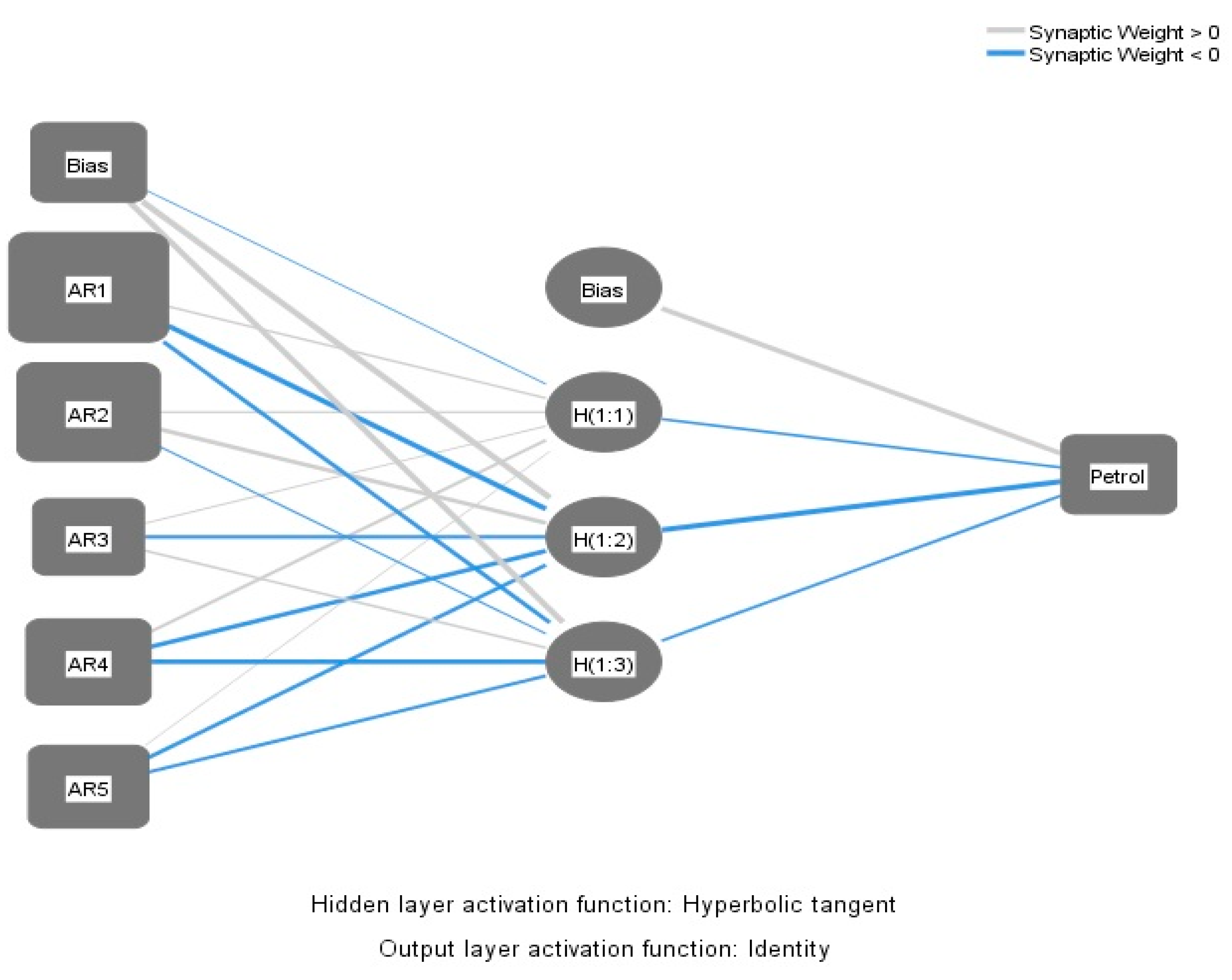
| Predictors | Parameter Estimates | ||||
|---|---|---|---|---|---|
| Hidden Layer 1 | Output Layer | ||||
| H (1:1) | H (1:2) | H (1:3) | Petrol | ||
| Input layer | AR1 | 0.205 | −1.019 | −0.673 | |
| AR2 | 0.091 | 0.756 | −0.086 | ||
| AR3 | 0.085 | −0.557 | 0.219 | ||
| AR4 | 0.354 | −0.757 | −0.773 | ||
| AR5 | 0.018 | −0.636 | −0.441 | ||
| Bias | −0.069 | 1.759 | 1.757 | ||
| Hidden layer 1 | H (1:1) | −0.287 | |||
| H (1:2) | −1.593 | ||||
| H (1:3) | −0.338 | ||||
| Bias | 1.015 | ||||
| Model training | SSE = 1.644 | ||||
| Model testing | SSE = 0.422 | ||||
| t-value | t = 0.917 | ||||
| p-value | p = 0.362 | ||||
| Series | Model | MAPE |
|---|---|---|
| AR1 | ARIMA(0,1,3)(0,1,1)4 | 1.813 |
| ARIMA(0,1,1)(0,1,1)4 | 1.651 | |
| ES(AHW) | 1.260 | |
| ES(MHW) | 1.556 | |
| AR2 | ARIMA(0,1,0)(2,0,0)4 | 0.922 |
| ARIMA(0,1,0)(0,0,2)4 | 0.794 | |
| ES(AHW) | 0.395 | |
| ES(MHW) | 0.650 | |
| AR3 | ARIMA(0,1,0)(0,1,0)4 | 1.020 |
| ARIMA(0,1,0)(4,1,0)4 | 2.318 | |
| ES(AHW) | 1.211 | |
| ES(MHW) | 1.130 | |
| AR4 | ARIMA(1,1,0)(0,1,0)4 | 0.501 |
| ARIMA(0,1,1)(0,1,0)4 | 0.446 | |
| ES(AHW) | 0.748 | |
| ES(MHW) | 0.809 | |
| AR5 | ARIMA(0,1,0)(0,1,1)4 | 0.853 |
| ARIMA(0,1,0)(0,1,0)4 | 1.213 | |
| ES(AHW) | 0.917 | |
| ES(MHW) | 0.949 |
© 2019 by the authors. Licensee MDPI, Basel, Switzerland. This article is an open access article distributed under the terms and conditions of the Creative Commons Attribution (CC BY) license (http://creativecommons.org/licenses/by/4.0/).
Share and Cite
Zhao, L.; Liu, Z.; Mbachu, J. Energy Management through Cost Forecasting for Residential Buildings in New Zealand. Energies 2019, 12, 2888. https://doi.org/10.3390/en12152888
Zhao L, Liu Z, Mbachu J. Energy Management through Cost Forecasting for Residential Buildings in New Zealand. Energies. 2019; 12(15):2888. https://doi.org/10.3390/en12152888
Chicago/Turabian StyleZhao, Linlin, Zhansheng Liu, and Jasper Mbachu. 2019. "Energy Management through Cost Forecasting for Residential Buildings in New Zealand" Energies 12, no. 15: 2888. https://doi.org/10.3390/en12152888
APA StyleZhao, L., Liu, Z., & Mbachu, J. (2019). Energy Management through Cost Forecasting for Residential Buildings in New Zealand. Energies, 12(15), 2888. https://doi.org/10.3390/en12152888