Simultaneous Inertia Contribution and Optimal Grid Utilization with Wind Turbines

Abstract

This paper presents findings of a study on continuous feed-in management and continuous synthetic inertia contribution with wind turbines. A realistic case study, based on real measurements, is outlined. A wind turbine feeds into a weak feeder, such that its power has to be adapted to the permissible loading of this feeder. At the same time the wind turbine is to provide inertia to the grid by applying the previously published variable inertia constant controller. It is discussed that optimal grid utilization and simultaneous inertia contribution are mandatory for the frequency control in power systems that are heavily penetrated with renewable energies. The study shows that continuous feed-in management can be combined well with continuous inertia provision. There are hardly any negative consequences for the wind turbine. The benefits for the grid are convincing, both in terms of increased system utilization and in terms of provided inertia. It is concluded that wind turbines can enhance angular stability in a power system to a larger extent than conventional power plants.

1. Introduction

In the transition to renewable energy, wind turbine (WT) generators substitute conventional power plants. Therefore, WTs must no longer merely behave like passive power sources; instead, they have to take over grid stabilizing functionalities that were traditionally carried out by conventional power plants.

The intermittent power infeed of WTs and the dispersed installation of WTs in the grid lead to temporary congestions in the grid and/or costly grid extensions. Germany, particularly the state of Schleswig-Holstein in the very north of Germany, is a prime example for this development [1,2]. In order to minimize the costs for grid extensions the power infeed of WTs should be matched to the maximum permissible power transfer capability of the affected part of the grid [3]. For this purpose, continuous feed-in management (FIM) was proposed in the past [4]. It was shown that continuous FIM allows maximizing the utilization of the grid and, consequently, maximizing the wind energy yield [5]. However, both during conventional FIM (as it is state of the art today [6]) as well as during continuous FIM, the control of a WT is partly decoupled from the wind speed. Hence, the stress on the WT increases.

Another task that WTs have to take over when conventional power plants are replaced is the contribution to grid inertia, which aims at stabilizing the grid frequency. Here, it has to be mentioned that different approaches are conceivable, which can be categorized into fast frequency response and synthetic inertia [7]. In this paper, the provision of synthetic inertia is in the focus for reasons outlined below. Also inertia contribution partly requires decoupling the controls of a WT from the instantaneously prevailing wind. Therefore, the stress on the WT potentially increases even more, depending on the control strategy and the wind condition. Load simulations and field measurements show that there is no negative effect on the ultimate loads to be expected, but fatigue loads are bound to increase [8,9].

The study on continuous FIM with a fictitious controllable WT (mentioned above) was based on measurements of wind speed, local consumption, and the passive wind power infeed of a real WT without grid support functionalities. Since the grid frequency was also measured, this study was extended to inertia provision with the controllable WT. Hence, the considered WT has to adjust its instantaneous power to not only fit the loading of the affected grid components, but also to the rate of change of frequency (ROCOF) in the grid, in order to provide the grid with synthetic inertia.

At first sight, the combination of continuous FIM and continuous provision of synthetic inertia seems random. Comparing the priorities that are set in the context of power system stability, it seems obvious that angular stability comes first and any secondary aspects, such as thermal loading of grid components or overvoltages, are of minor importance [10]. However, in a power system that is heavily penetrated with dispersed renewably energy sources, the traditional rules are no longer applicable. For economic reasons, grid connection of dispersed renewable energy generation develops slower, and often not to the same extent, as the installation of the generators. Consequently, the power infeed of these generators has to be restricted in weather situations that allow the production of large amounts of renewable power [5,11]. The transition to renewable energies is only economically feasible if conventional power plants are replaced; i.e., if they do not have to remain in standby, waiting to step in if renewable energy infeed is insufficient. This means that the availability of renewable power infeed must not be unduly hampered by the transfer capabilities of grid components, as this would interfere with the balance between generation and demand; i.e., continuous FIM is mandatory as it interacts with grid frequency control. At the same time, replacing conventional generation (based on AC connected rotating machines) with frequency converter-based renewable energy generators leads to a decline in inertia in the power system. However, power system inertia is essential for the control of the frequency, i.e., the balance between generation and demand [12,13]. There is no consensus whether frequency converter-based generation should enhance grid frequency control by contributing to the grid inertia continuously, or by responding to predefined frequency events in a predefined manner (fast frequency response). Some scientists advocate fast frequency response and even deem continuous provision of synthetic inertia to be inappropriate [14]. Different grid codes prefer fast frequency response; others demand continuous provision of synthetic inertia by emulating the inertial behavior of synchronous generators [15,16,17,18]. In future power systems, where frequency converter-based generation substitutes almost all AC connected rotating machines (i.e., very low natural inertia), continuous provision of synthetic inertia is mandatory. Consequently, the simultaneity of continuous FIM and continuous provision of synthetic inertia is inevitable.

In this study, the assessed WT is enhanced to continuously provide inertia, comparable to a synchronous generation of a conventional power plant. To avoid the risk that the WT disconnects from the grid when during low wind speeds a large negative ROCOF requires a large increase in power, the previously proposed variable inertia constant (H_var) controller [19] is applied.

In the following sections, first, the case study is outlined. Secondly, the WT simulation model with its different controllers is introduced. A frequency domain analysis compares the response of the WT to the demanded continuous inertia provision and the continuous FIM. It is outlined that the prioritization mentioned above: 1st priority is inertia contribution, 2nd priority is addressing grid congestions (FIM) is implemented in the proposed controllers. Hence, the simultaneous coexistence of synthetic inertia and continuous FIM is facilitated. Finally, simulation results prove that combining continuous synthetic inertia with continuous FIM is no problem for the affected WT and that it is a big gain for the grid.

2. Case Study

The university campus in Flensburg, Germany, is a small power system that comprises consumption, generation, and a connection to the external grid. For the purpose of this study, the campus grid is assumed to be supplemented by a 5 MW WT and the connection to the external grid is assumed to be made of an oil-immersed transformer whose rating is sufficient only most of the time. Hence, this study case replicates the situation that commonly occurs when wind power grows faster than the power system into which the WTs feed their power. The NREL 5 MW reference turbine is chosen for this extension, and is called 5M in the following, as the details of this WT are well documented and openly accessible [20]. The 5M is represented with a simulation model that exhibits the most dominant vibratory behaviours of a WT: the first eigenmodes of the tower, the drive train, the rotor blades in edgewise direction, and the rotor blades in flapwise direction [21]. This model is chosen because it is easy to implement and use. Also, it can be easily extended with grid models and additional controllers.

Figure 1 shows a sketch of the Flensburg university campus with the supplements necessary for this case study. It can be seen that already, today, the local consumption is partially covered by the power of a WT on campus, which is an Enercon E30, whose power is indicated as P_E30 in Figure 1. In this case study, the residual load, which either has to be covered by the 5M, or by power import from the external grid, is called P_C (see Figure 1).

For this study P_C, P_E30, wind speed, grid frequency, f_grid, and the ambient temperature were measured on 05 April 2017, which was a day with changing and eventually quite good wind conditions and a typical load profile for the campus. The measurements of P_C, P_E30, wind speed, and the ambient temperature are already published [5]; hence, they are not reproduced here.

For the assessment of inertia contribution, the measurement of the grid frequency, f_grid, is essential [22]. Therefore, Figure 2 shows f_grid, the calculated ROCOF and the frequency spectrum of f_grid and the ROCOF as measured on 5 April 2017.

Figure 2 reveals that the ROCOF the WT has to respond to is very small most of the time, (|ROCOF| < 0.02 Hz/s). However, there are some single peaks, the largest even reaches −0.484 Hz/s. These peaks are only a rarely occurring phenomenon. It is not clear where these peaks come from; however, their frequency of occurrence, their durations, and their magnitude suggest that they are not of electromechanical nature. It is rather assumed that distortions in the grid voltage lead to these large ROCOFs. Previously conducted research revealed this effect and quantified the number of fake ROCOF incidences, i.e., occurrence of large ROCOF values that are not of electromechanical nature, but that are caused by electromagnetic effects [23]. Instead of eliminating these fake ROCOF values, they are deliberately left in the time series. If a real WT has to perform inertial response it has to measure the voltage to determine the frequency and the ROCOF in real-time. In such online computation of the ROCOF, a distorted grid voltage will also lead to large values. This is particularly important for the WT, as it can have noticeable effects on the mechanical loads, and hence, on the fatigue of the WT.

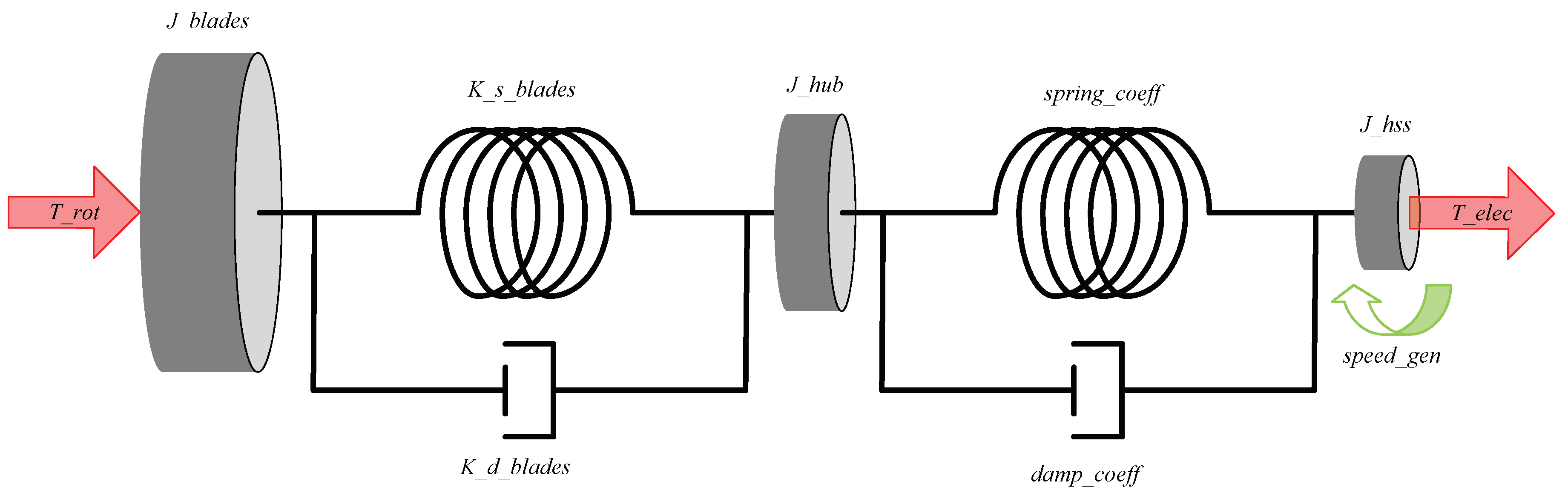
3. WT Simulation Model

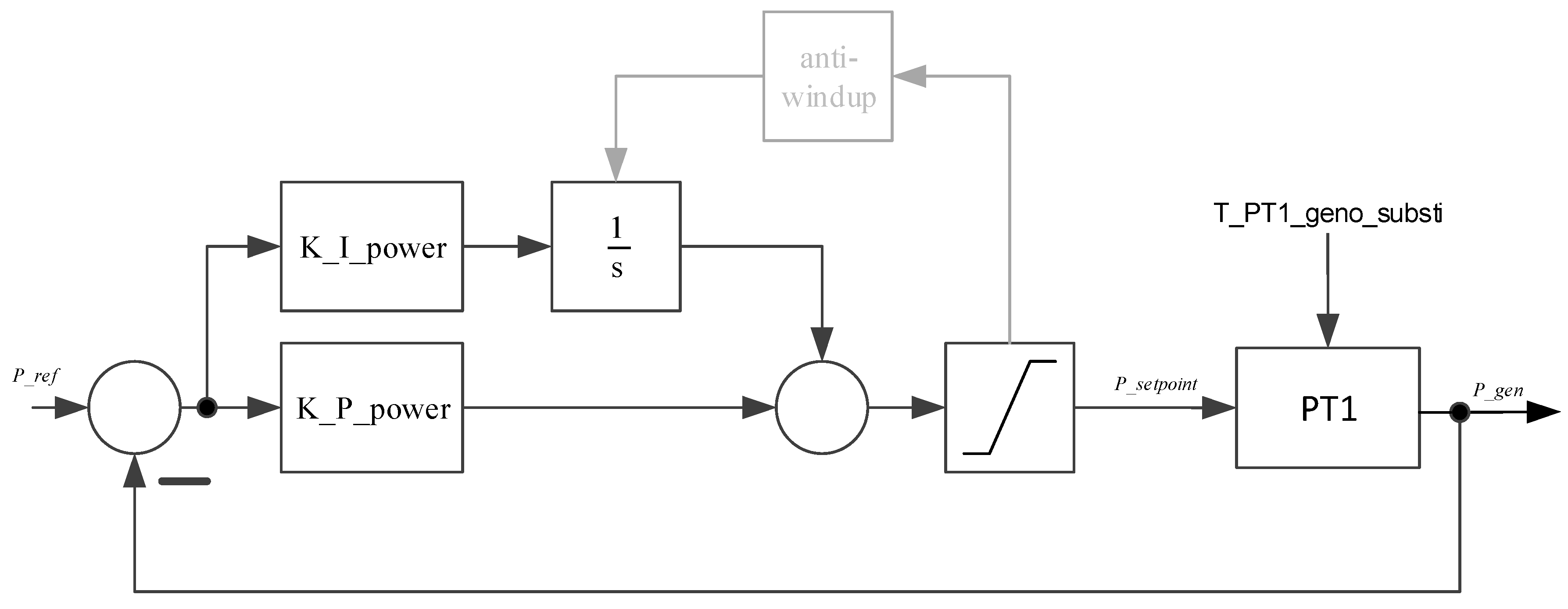
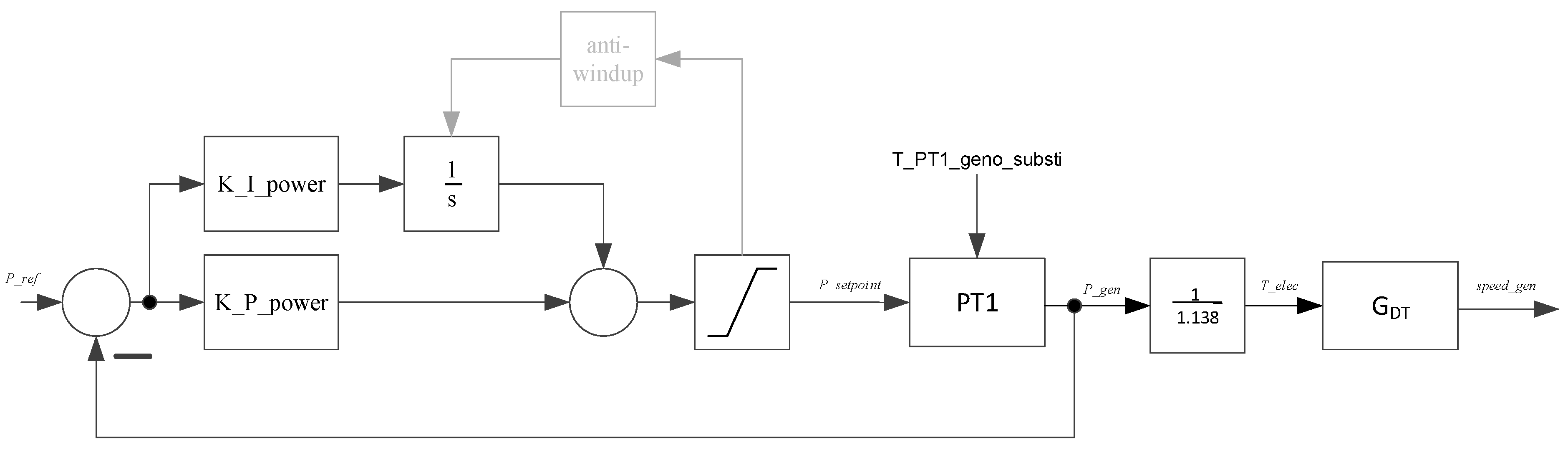
3.1. Power Controller

The 1st eigenmodes model of a WT represents the generator–converter unit as a first order low pass filter (PT1). This means that the dynamics of the generator, the machine side inverter, the grid side inverter, as well as the capacitor in the DC circuit are modelled as one lumped PT1 element. In the previous study on continuous FIM [5], the time constant of this PT1 filter (T_PT1_geno_substi [21]) was set to 150 ms, which is a reasonable value for normal power control of a WT. In the inertial response study shown here, this time constant has to be reduced to a lower, yet realistic value, to allow more rapid power variations as this is needed for effective inertial response. Hafiz and Abdennour propose a time constant of 20 ms for a multi-MW generator–converter unit [24]. In a Bachelor thesis composed at WSTECH GmbH, which is a manufacturer for frequency converters, a PT1 response with a time constant of 25 ms was applied for simulating the power response of MW frequency converters [25]. Hence, in this study, T_PT1_geno_substi is set to 25 ms (T_PT1_geno_substi = 0.025 s) as this is more conservative and facilitates running the simulation with a simulation time step of dT = 0.001 s. A smaller simulation time step would lead to computational problems as the scenario to be assessed lasts 24 hours. Hence, the amount of data resulting from such long time series becomes very large and Matlab [26], which is the software with which the simulations are conducted, can no longer handle this amount of data on a normal personal computer.

Figure 3 shows the power control loop with the PI power controller and the PT1 filter that represents the generator–converter unit. The aforementioned reduction of T_PT1_geno_substi causes the open loop power control path to exhibit a higher crossover frequency; compare the green and the dashed blue curve in the bode plot in Figure 4. A higher crossover frequency allows rapid power variations to pass through with less damping, which causes the PI controller to exhibit overshoots. Overshooting of the controller leads to hitting the controller output limitations and triggers the anti-windup facility of the I-part of the PI controller [21]. The anti-windup block is shown in grey in Figure 3 as it is normally not involved in power control operation. Consequently, the gains of the PI controller are tuned to restore the initial crossover frequency of about 12 Hz. This is achieved with the proportional gain K_P_power = 2.1 and the integral gain K_I_power = 12. With these gains, the phase margin increases to about 109 degrees, see Figure 4, which proves stability. However, stability is not the problem to be dealt with here. Instead, a large phase margin is required in order to avoid oscillations and overshoots, which would trigger the anti-windup of the integrator. Although the anti-windup facility prevents numerical instability, excessive triggering of it can lead to numerical oscillations between the upper and the lower controller output limits. Such numerical oscillations lead to wrong results. With these parameter settings, the transfer function of the open power control loop is given in Equation (1).

$$G_{P\_cntrl\_OL}\left(s\right)=\frac{P_{gen}\left(s\right)}{P_{ref}\left(s\right)}= \frac{0.7·s+2.1}{0.008333·s^2+0.3333·s}$$

(1)

3.2. Continuous Feed-In Management Control

The power generated by the 5M is first and foremost determined by the prevailing wind speed. Whenever the power approaches rated power, the transformer that connects the campus grid with the upstream grid is bound to get overloaded. This overload appears in the shape of overheating of the transformer (ϑ_TR) and too high voltage, V_C, in the campus grid (see Figure 1). Consequently, FIM becomes necessary in situations of high wind speeds, and/or very low local consumption in the campus grid. The FIM controller, which is shown in Figure 6 addresses the thermal loading of the transformer as well as V_C [5].

3.3. Continuous Inertial Response Control

The previously proposed variable inertia constant (H_var) controller has numerous advantages [19]. The main motivation for this controller is that WTs can continuously contribute to the inertia in the power system, without running the risk that drastic negative ROCOFs lead to disconnections of the WT. In principle, a WT with the H_var controller behaves like a synchronous generator. However, unlike a synchronous generator, the rotational speed of a WT is not constant. In an AC-connected synchronous generator, the rotor speed varies with f_grid. Since in most power systems f_grid varies only in a very narrow band, the rotational speed of AC connected synchronous generators can be considered almost constant. In a WT, however, the rotational speed is not determined by f_grid, but by the wind speed. Hence, it can vary in a wide range. Therefore, the H_var controller varies the inertia constant, which is emulated by the WT, according to the current rotational speed, see Figure 5. At rated speed, the variable inertia constant is equal to the value demanded by the grid operator (H_dem).

Equation (2) shows the definition of the inertia constant as known from the literature [10].

$$\mathrm{H}=\frac{E_{kin}}{P_{rated}}=\frac{\frac{1}{2}·J·{\omega }_{rated}^2}{P_{rated}}$$

(2)

Based on this concept, the H_var controller defines an inertia constant for every prevailing rotational speed [9]:

$$H_{var}=\frac{{\omega }^2- {\omega }_{cut-in}^2}{{\omega }_{rated}^2- {\omega }_{cut-in}^2}·H_{dem}$$

(3)

Figure 5 reveals the main advantage of the H_var controller: Since the inertia contribution drops to zero when the rotational speed is as low as the cut-in speed, the WT never disconnects from drastic negative ROCOFs. At low wind speeds (i.e., also low rotational speed and low power), a single WT provides little inertia. However, this seeming disadvantage is not a problem for the grid: in such a situation, the prevailing load is either supplied by a larger number of WTs (which in total supply sufficient inertia) or by other generators, which can also supply the needed inertia. Equation (2) and Equation (3) reveal that the contributed inertia is scaled with the current speed and therefore also with current power infeed of the WT. Hence, if low wind speed allows one WT to produce only little power, then the overall load in the grid has to be covered by a larger number of WTs. This automatically distributes the generation of H_dem over all WTs that are equipped with an H_var controller. In total the grid is supplied with the inertia that the grid operator demands.

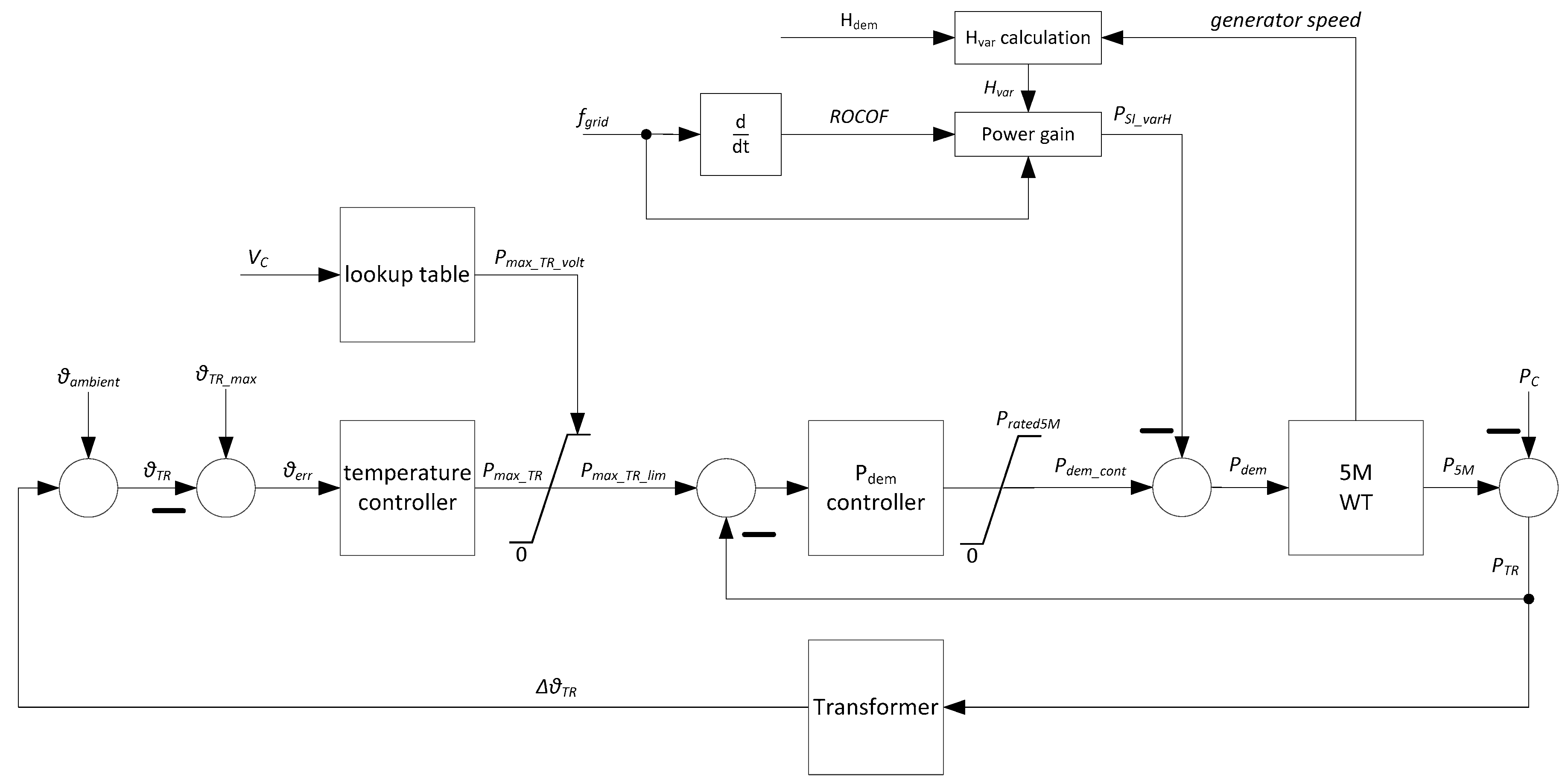
3.4. Combined Control Circuit

Both, the continuous FIM controller and the H_var controller interact with the 5M WT via the power setpoint, P_dem. Figure 6 illustrates that the continuous FIM controller responds to the transformer temperature, ϑ_TR, and the voltage in the campus grid, V_C. The H_var controller generates the H_var from the demanded inertia constant, H_dem, and the generator speed. The inertial response power setpoint, P_{SI_varH}, is a result of the ROCOF, f_grid and the current H_var, see Equation (4) [19].

$$P_{SI\_varH}=-2·H_{var}·P_{rated}·\frac{ROCOF}{f_{grid}}$$

(4)

In the version of the 1st eigenmodes model applied here, P_dem has no impact on the rotational speed reference of the WT. Hence, even with P_dem < 1 pu, the speed of the WT reaches rated speed if the wind speed suffices [21]. This characteristic is beneficial for continuous inertia provision, as it allows the WT to produce H_dem for a maximum duration.

FIM and inertial response do not only decouple the controls of a WT from the prevailing wind at the rotor. Since they both act on P_dem, they could, potentially, also interfere with each other. However, Figure 6 shows that they are decoupled from each other by the different controllers. Due to the long thermal time constant of the transformer, the temperature controller lets P_{max_TR} respond only very slowly. P_{max_TR_volt} has an instantaneous effect on P_{max_TR_lim}. This variable only serves as setpoint for the P_dem controller, which is tuned to fit the vibratory behaviour of the WT. P_{SI_varH}, however, acts instantaneously on P_dem. With this configuration, inertia contribution is clearly prioritized over FIM. Even if P_{SI_varH} leads to V_C violating any limits, this can only impact on the power output of the WT via the dynamics of the P_dem controller. This prioritization is justified, as power from inertia contribution oscillates around zero. Hence, it has no lasting impact on the transformer temperature. However, if inertial power is essential for maintaining angular stability, violations of voltage limits are of subordinate importance. This is discussed further in the section on frequency domain analysis.

It has to be noted that the H_var controller was initially published with a functionality to mitigate potentially harmful excitations on the mechanical structure of the WT [19]. This functionality is deliberately omitted here to be able to assess the maximum inertial response capabilities. At the same time, it is the goal of this paper to reveal the maximum negative impact of inertial response on the WT. Hence, the worst case scenario is considered here.

While in this paper all explanations are given for the case of one WT only, the same result could be realized with an arbitrary number of WTs. As described above, the H_var controller inherently distributed the inertial power generation among any participating generators. Even in a wind farm, where wake effects lead to grossly differing operating points of neighbouring WTs, the H_var controller assures that the inertia contribution of individual WTs is adapted to their instantaneous capabilities.

The FIM controller, on the other hand, does not take the current operating point of a WT into account. It could be assumed that what is called 5M in Figure 1 is not a single WT, but a wind farm with multiple WTs that interfere with each other via wake. Since all these WTs would contribute to the congestion in the point of common coupling (excessive transformer temperature and too high voltage), they would respond to this congestion equally. This would not be ideal, as the instantaneous power operating points of the individual WTs would differ due to wake and due to the natural wind speed variations in time and space. Also, due to the spatial distribution of the individual WTs in the wind farm, the cable lengths to the point of common coupling would be different. Hence, the voltage drops and the power losses in these cables would be different. Consequently, the task of FIM should be distributed among the different WTs taking the wind direction (wake) and the geometry of the wind farm (beelines and cable lengths) into account. However, the design of such an FIM wind farm controller is beyond the scope of this paper.

4. Frequency Domain Analysis

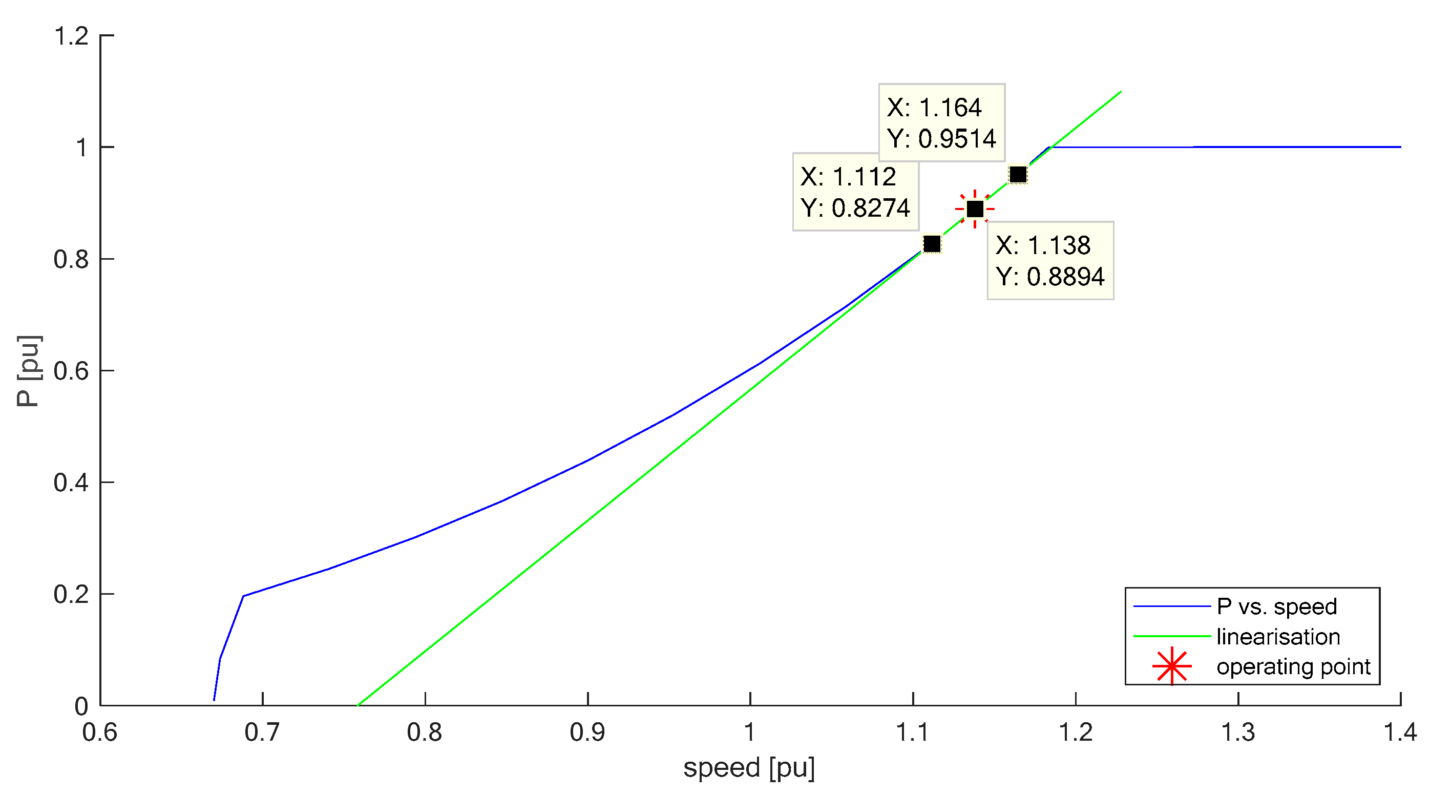
4.1. Transfer Function of WT

In contrast to assessing the different eigenfrequencies, as they result from the design of the 5M [27], in this section, a frequency domain analysis is presented. This yields the advantage that the frequency response of the entire system becomes obvious. In a complex system, eigenfrequencies of adjacent subsystems can couple and consequently interfere. The controller design described above has an impact on the eigenfrequencies and damping of different subsystems of the WT system. In the power controller section, the assumption is made that the power of the generator, P_gen, is independent of the rotational speed. This assumption is only valid in the case of small signal perturbation. Hence, in the following, the response of the rotational speed to power variations is assessed.

For the purpose of frequency domain analysis, the WT system is linearized around the upper part load operating point P = 0.8894 pu and generator speed, speed_gen = 1.138 pu, see Figure 7. It has to be noted that Figure 7 shows the power vs. speed characteristic that results from the aerodynamics of the 5M when the 5M is assumed to be equipped with a full scale converter. In contrast to a doubly fed induction generator, a full-scale converter allows the WT to operate in a considerably larger speed band.

Upper part load is most interesting: In lower part load, the power of a WT is not likely to cause FIM as it is too low for causing the transformer to heat up unhealthily, or for running the voltage into its limit. Also, in lower part load, i.e., low rotational speed, the power resulting from inertial response is small due to the H_var controller, see Figure 5. Full load, on the other hand, is also less interesting as this operating point is only seldomly met when the grid connection capabilities demand FIM. In addition, inertial response can draw extra power from the wind when the WT is in full load operation; hence, the impact on the speed is not decisive for the power.

The rotational speed responds whenever there is a mismatch between aerodynamic driving power and electric output power. Such a mismatch has to be catered for by kinetic energy in the rotating masses of the WT. Hence, a transfer function of the WT drive train from electric torque to rotational speed of the generator, speed_gen, is required. High frequency variations in the generator torque (T_elec) mainly act on the energy storages close to the generator; i.e., the inertia on the high speed shaft, J_hss, the torsional spring that represents the stiffness of the drive train, spring_coeff, and with decreasing effect also the inertia of the hub, J_hub, and the spring that represents the blades in in-plane direction, K_s_blades (Figure 8). Therefore, the aerodynamic operating point is considered constant for the linearization of the operating point.

In the WT model applied here, the blades are represented as single mass and spring vibrators. However, they behave differently only if they are excited differently [21]. Wind speed and rotor position vary with time. In order to do the transition to the frequency domain, these time-dependent differences are neglected, which allows considering the blades to vibrate synchronously. This simplification leads to the rotational system of the WT as shown in Figure 8.

The variable names and parameter names shown in Figure 8 and in the following equations are identical with those in the documentation of the model [21]. Differing from the model documentation, some new parameters are introduced in Figure 8, which result from the simultaneity of the aforementioned blade motion. These new parameters are introduced in the following equations.

Aggregated blade inertia:

$$J\_blades = \frac{m\_bladetip·3·\left(R\_cntr\_gravi\_bladetip\right)²}{J\_base\_lss}$$

(5)

Aggregated blade stiffness:

$$K\_s\_blades = \frac{K\_s\_blade\_inplane\_SI·3}{J\_base\_lss}$$

(6)

Aggregated blade damping:

$$K\_d\_blades = \frac{K\_d\_blade\_inplane\_SI·3}{J\_base\_lss}$$

(7)

Inertia aggregated in the rotor hub:

$$J\_hub = \frac{J\_hub\_SI + 3·J\_bladeroot}{J\_base\_lss}$$

(8)

Since part load operation is assumed, the pitch angle is assumed to be constant at approximately 0°. Therefore, the stiffness in-plane (K_s_blade_inplane_SI) is the edgewise stiffness and the damping in-plane (K_d_blade_inplane_SI) is the edgewise damping of the blades.

Applying free-body diagrams for the inertias shown in Figure 8 allows deriving the transfer function of the drive train from generator torque (T_elec) to generator speed (speed_gen), where T_elec is the input variable and speed_gen is the unknown [28]. For this purpose a constant aerodynamic driving torque, $T\_rot =\frac{P}{speed}$ = 0.7815 pu is applied according to the previously specified operating point (Figure 7).

The transfer function from torque to speed of the WT is shown in Equation (9).

$$G_{DT}\left(s\right)=\frac{speed\_gen\left(s\right)}{T\_elec\left(s\right)}= \frac{-15.02·s^5-9.405·s^4-2509·s^3-1031·s^2+7.276E\left(-12\right)·s}{17.59·s^6+32.77·s^5+4670·s^4+7045·s^3+2.577E5·s^2+1.827E5·s-1.456E\left(-9\right)}$$

(9)

It has to be noted that other dynamics in the WT, i.e., dynamics of the tower and of the blades in out of plane direction, can be neglected. These dynamics have no direct coupling with the rotational speed. There is only an indirect coupling via the perceived wind speed and the aerodynamics of the rotor blades, which has only a small influence on the generator speed, compared to the effects of in-plane vibrations.

The transfer function of the drive train, G_DT(s), can be combined with the transfer function of the power control loop to form the transfer function from P_ref to speed_gen, G_WT(s). For this purpose, G_{P_cntrl_OL}(s) in Equation 1 has to be turned into the transfer function of the closed power control loop. Linearization around the operating point speed_gen = 1.138 pu allows setting up the block diagram of G_WT(s), as shown in Figure 9.

The complete transfer function from P_ref to speed_gen is shown in Equation (10).

$$G_{WT}\left(s\right)=\frac{speed\_gen\left(s\right)}{P\_ref\left(s\right)}=\frac{-0.08759·s^7-3.821·s^6-27.5·s^5-641.9·s^4-2015·s^3-721.5·s^2+5.093E\left(-12\right)·s}{0.001222·s^{10}+0.2026·s^9+7.064·s^8+77.85·s^7+1811·s^6+8767·s^5+1.003E05·s^4+2.465E05·s^3+1.279E05·s^2-1.019E\left(-9\right)·s}$$

(10)

4.2. Transfer Function of Transformer

The thermal behaviour of the transformer is represented by a PT1 filter with a time constant of 960 s. The power losses that heat up the transformer are nonlinearly depending on the power that is fed through the transformer. Therefore, the transformer is linearized around the operating point 0.1 pu power transfer, as this is a realistic maximum extent of inertial power. Since only the interference between FIM and inertia contribution are assessed, the steady state operating point of the transformer is irrelevant. Further considering the heat dissipation at the surface of the transformer leads to the power that is stored in the transformer in the form of heat [5]. Hence, the transfer function from power transfer in pu to variation in the transformer temperature in °C is given in Equation (11).

$$G_{TR}\left(s\right)=\frac{\Delta {\vartheta }_{TR}\left(s\right)}{P_{TR}\left(s\right)}= \frac{5.005}{1+960·s}$$

(11)

4.3. Transfer Function of P_dem Controller

The P_dem controller is a PI controller with a proportional gain of three and an integral gain of nine. The P_dem controller is the separator between FIM and inertia contribution; i.e., if inertial power leads to instantaneous violation of V_C, the P_dem controller prevents this having an instantaneous effect on the combined power setpoint, and hence, also the inertia contribution. Equation (12) shows the transfer function of the P_dem controller.

$$G_{PI\_P\_dem}\left(s\right)=\frac{P_{dem\_cont}\left(s\right)}{P_{error}\left(s\right)}= \frac{0.3333·s+2.1}{0.1111·s}$$

(12)

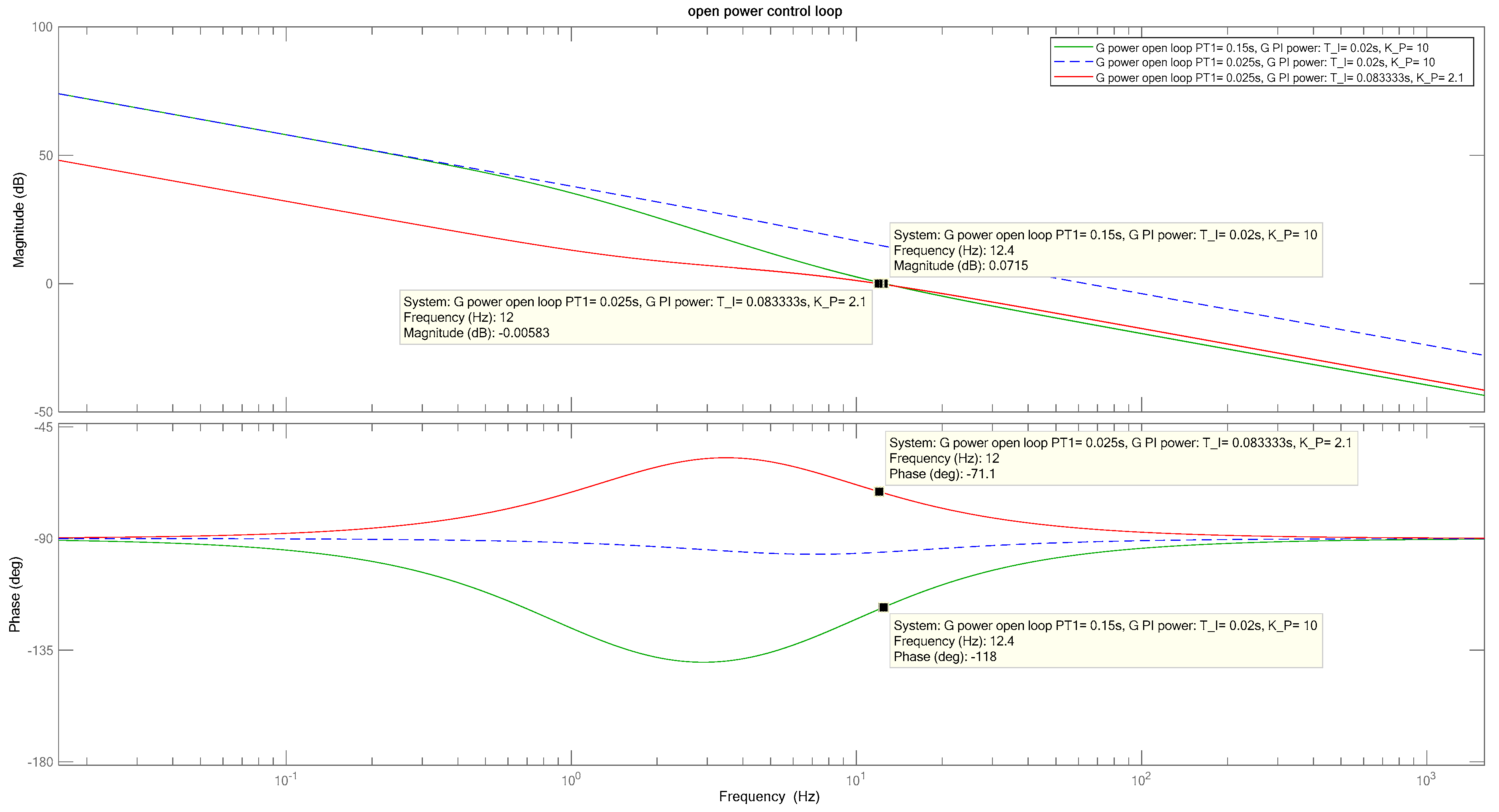
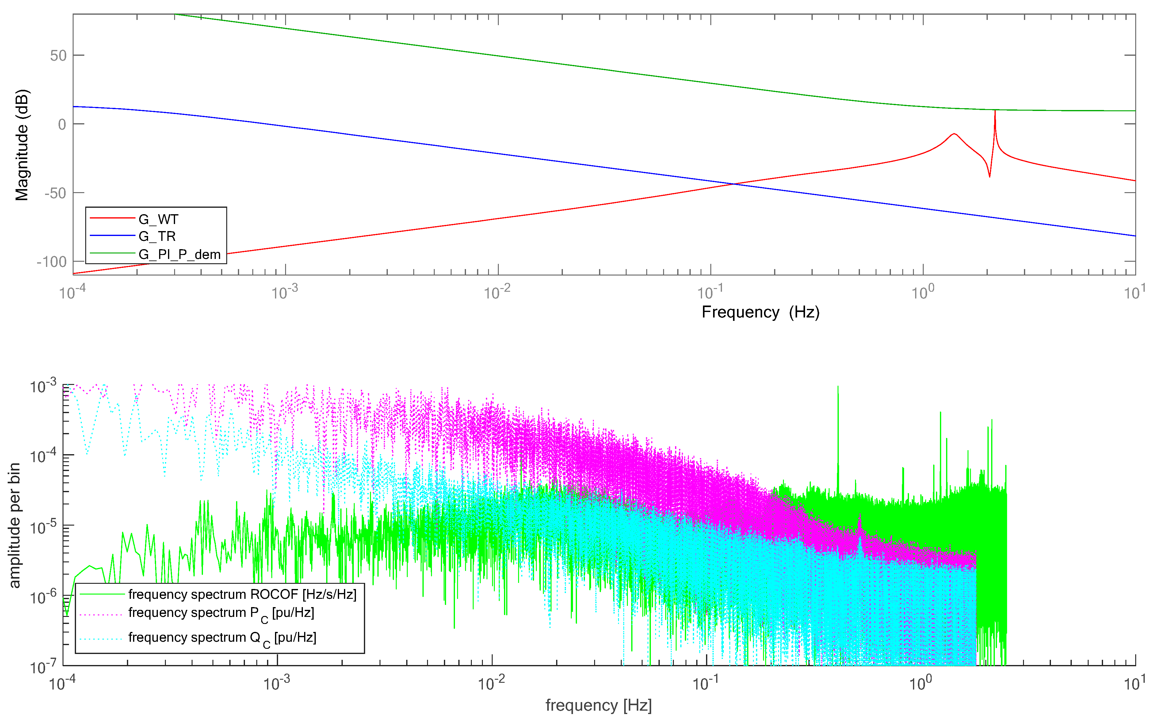
4.4. Comparison of Frequency Responses

In this section, the frequency responses of the transfer functions derived above are compared with the frequency spectra of the excitations. The excitations for inertia contribution are the ROCOF. Continuous FIM has to address the loading of the grid connection transformer; hence, it has to respond to the local active power consumption/production. The voltage in the campus grid, V_C, responds to not only the active power P_C and the power from the 5M, P_5M, but mainly to the local reactive power consumption/production, Q_C (see Figure 1). The importance of Q_C is shown by the ratio between reactance and resistance in the grid connection transformer, which is X/R = 3.84 [5].

The analysis conducted here strives to assess the differences and the similarities in the excitations for the 5M when performing continuous FIM and continuous inertia contribution. Normal operation, i.e., with neither of these power system services, was considered previously [5] and is hence out of the scope of this paper. Consequently, Figure 10 shows the bode plots of the WT, G_WT(s) (red amplitude response) of the P_dem controller, G_{PI_P_dem}(s), (green amplitude response) and of the transformer, G_TR(s), (blue amplitude response); as well as the frequency spectra of ROCOF (green line), P_C (magenta dotted line) and Q_C (cyan dotted line).

Figure 10 clearly shows that there is a strong decoupling between the WT and the transformer. The transformer temperature (G_TR(s)) responds strongly to very low frequencies only. The generator speed of the WT, however, responds to power setpoint (P_ref) changes strongest in the range from 1 Hz to 3 Hz (G_WT(s)).

In the lower diagram of Figure 10 it becomes obvious that there is also a clear decoupling between the excitations of FIM and of inertia contribution. Continuous FIM addresses the transformer temperature (discussed above) and the voltage (V_C). Both active and reactive power variations decline with increasing frequency. Hence, also the extent to which FIM has to respond to V_C declines with increasing frequency. In contrast to this, the magnitude of the ROCOF increases with frequency.

Figure 10 also shows that the P_dem controller decouples FIM very well from inertial power. Comparing the green lines in Figure 10 reveals that the response to ROCOF happens in a frequency range where the P_dem controller exhibits very small gain. Hence, if inertial power leads to excessive V_C FIM cannot respond to that, i.e., it cannot dampen the inertial power as the P_dem controller prevents this.

Therefore, it can be concluded that FIM takes place at lower frequencies while inertia contribution takes place at higher frequencies. In addition, continuous FIM is most relevant for the transformer temperature, while inertia contribution has the potential to excite the WT. In the following section, this is assessed by means of the study case.

5. Simulations and Discussion of Results

In power systems that are heavily loaded with wind power, it is inherent to FIM that it leads to drastic power reductions in WTs whenever the wind speed is high [5,11]. In addition, it is inherent to the H_var controller that it potentially leads to drastic power variations in the affected WT whenever the wind speed is high [19]. Hence, both continuous FIM and inertial response with the H_var controller are most dominant in upper part load. The inertial response can potentially worsen the overloading of the grid. Due to the decoupling from the wind both controllers add to the mechanical loads in the WT at the same time.

Figure 11 shows the power, the generator speed, and the pitch angle of the 5M for the whole day of 5 April 2017. It can be seen that the 5M runs in part load most of the time in the first half of the day. Before noon, the wind speed increases and with it also the loading of the grid [5]. Hence, in the second half of the day the 5M runs in rated operation whenever the FIM controller and the H_var controller allow it to. Figure 11 shows the simulated scenario for continuous FIM operation with enabled (blue) and disabled (red) continuous inertia contribution. The blue curve is hardly visible, as there is only little effect of inertial response on FIM operation.

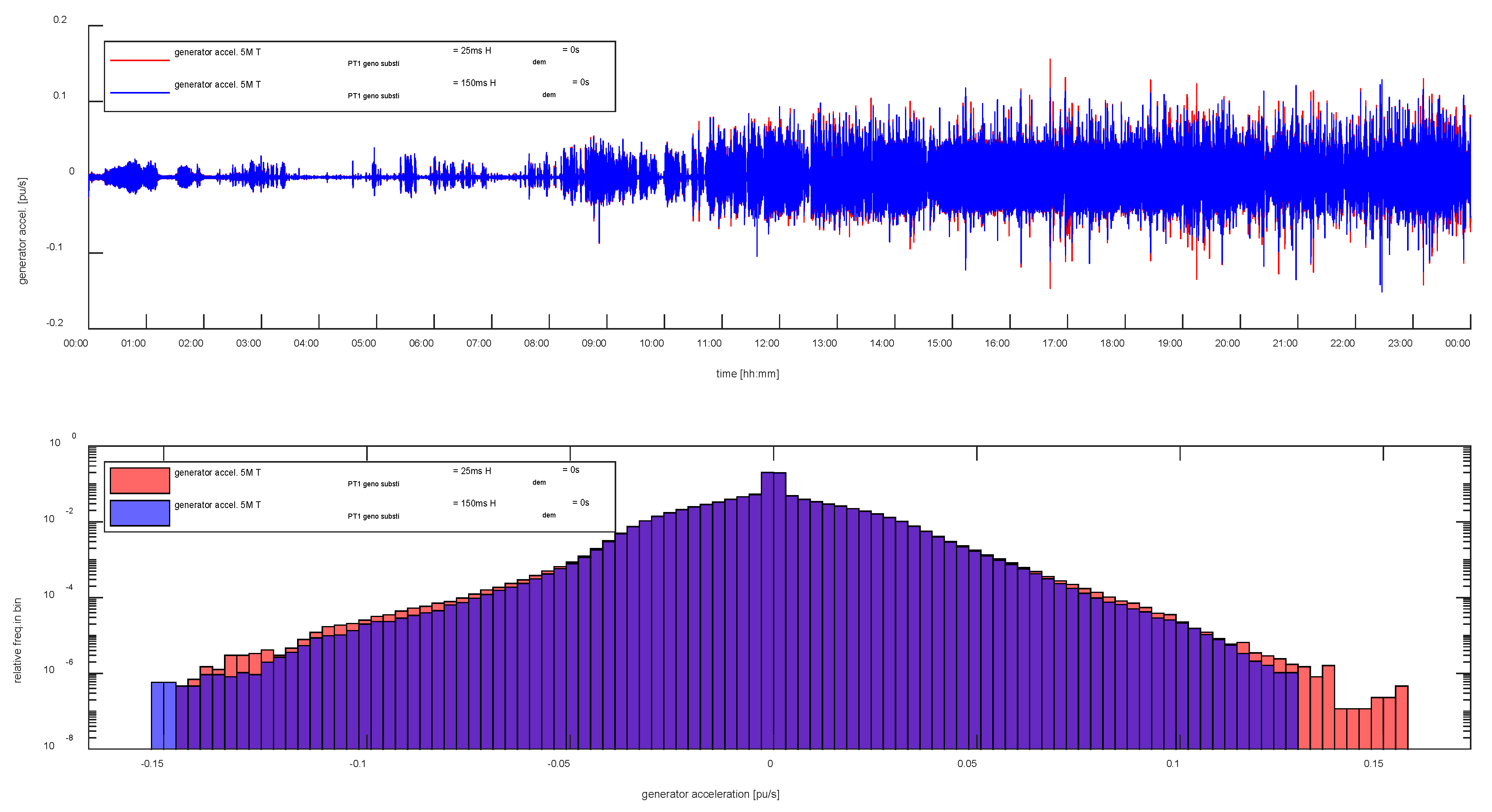
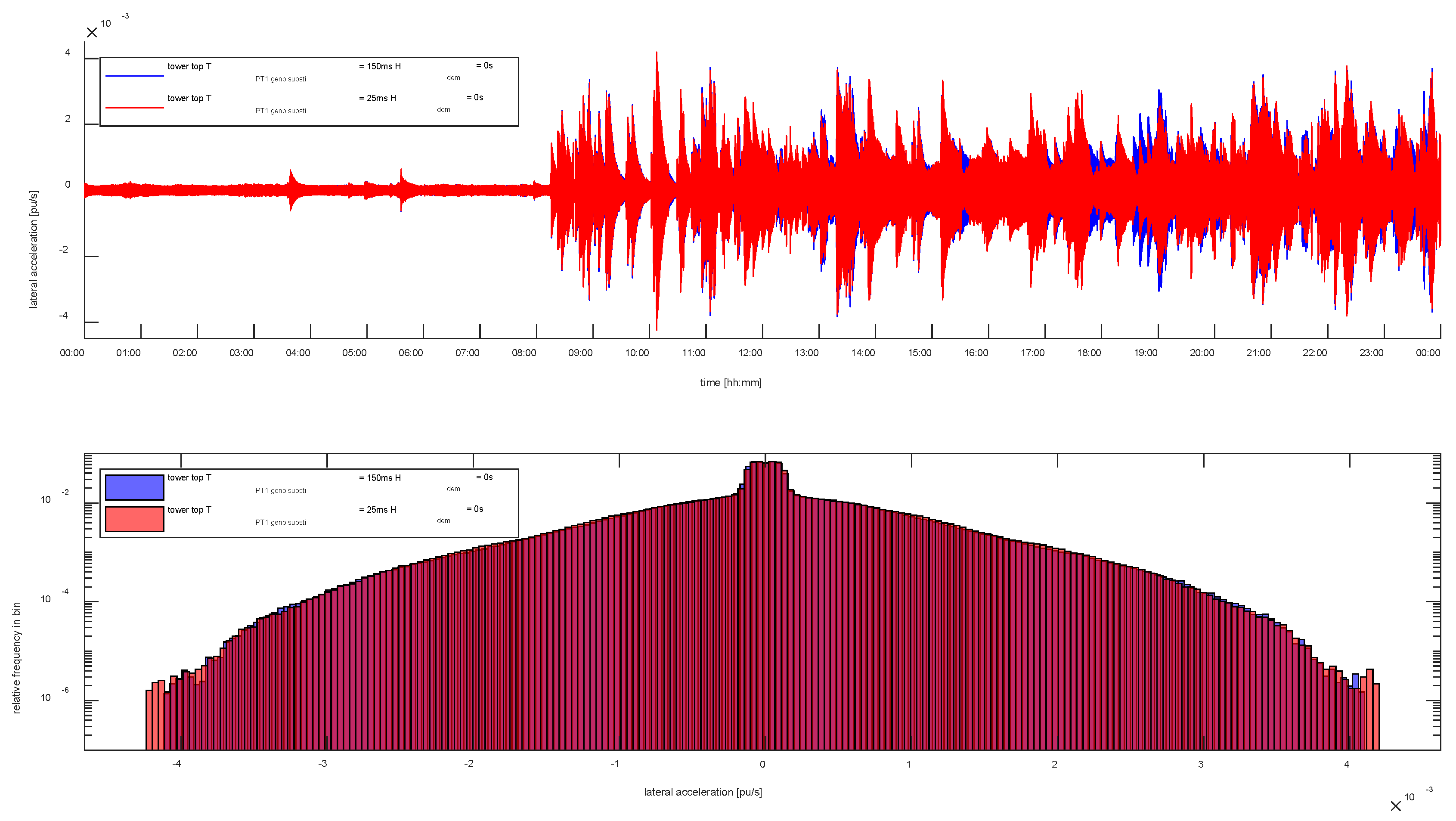
5.1. Effect of Generator–Converter Time Constant on Continuous FIM

As discussed in the WT simulation model section, in a previous study [5], T_PT1_geno_substi of the generator–converter unit was set to 150 ms. For reasons outlined above, it is set to 25 ms here. In order to assess whether the results in the previous paper are comparable to the results in this paper, the effect of the time constant is studied. It can be seen that the results presented previously [5] are hardly affected by this parameter change. The only visible effect is on the acceleration of the generator and of the tower in lateral direction. To illustrate this effect, Figure 12 shows the scenario of continuous FIM operation with T_PT1_geno_substi set to 150 ms [5] and with T_PT1_geno_substi set to 25 ms.

The comparison shown in Figure 12 is important as in the following study, the effect of continuous inertia provision is compared with the case when the WT only provides continuous FIM. Figure 12 suggests that the reduction in T_PT1_geno_substi (from 150 ms to 25 ms) has drastic consequences; however, due to the logarithmic scale, the relative frequency of occurrence of larger generator accelerations is moderate. It can be noted that with lower time constant, the relative frequency of occurrence is moved in positive direction, i.e., larger positive accelerations are more likely to occur. This phenomenon is caused by the instantaneous limitation of P_{max_TR_lim} whenever the voltage is too high (P_{max_TR_volt} in Figure 6), which demands a de-loading of the generator by lowering the generator torque.

Figure 13 shows that the reduction in T_PT1_geno_substi has the opposite effect on the lateral tower accelerations. With longer time constant, i.e., slower generator control, the tower is bound to vibrate more often in lateral direction. This phenomenon is due to the fact that lateral vibrations are caused by an imbalance in the rotor in combination with rotor speeds that allow lateral excitation of the tower by this imbalance. There is only an aerodynamic coupling between tower vibrations and the torque at the shaft (via the perceived wind speed). Faster generator control allows more rapid response of the generator by producing a counter torque. Hence, via the slope in the power vs. speed characteristic, the generator can produce more damping torque if its time constant is short.

Difference in acceleration of the other components in the 5M are hardly measurable. Consequently, the results presented previously [5] remain valid. Hence, it is justified that the effect of continuous inertial response on the WT is assessed against the case of continuous FIM with T_PT1_geno_substi set to 25 ms.

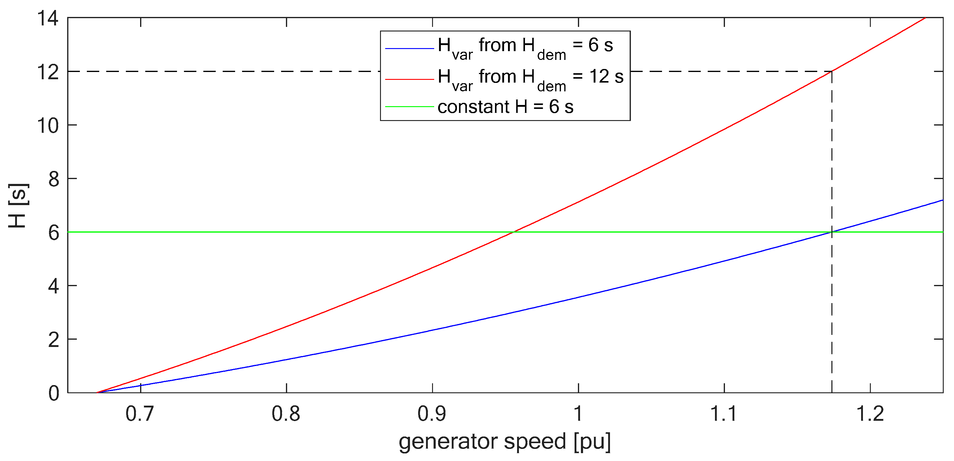
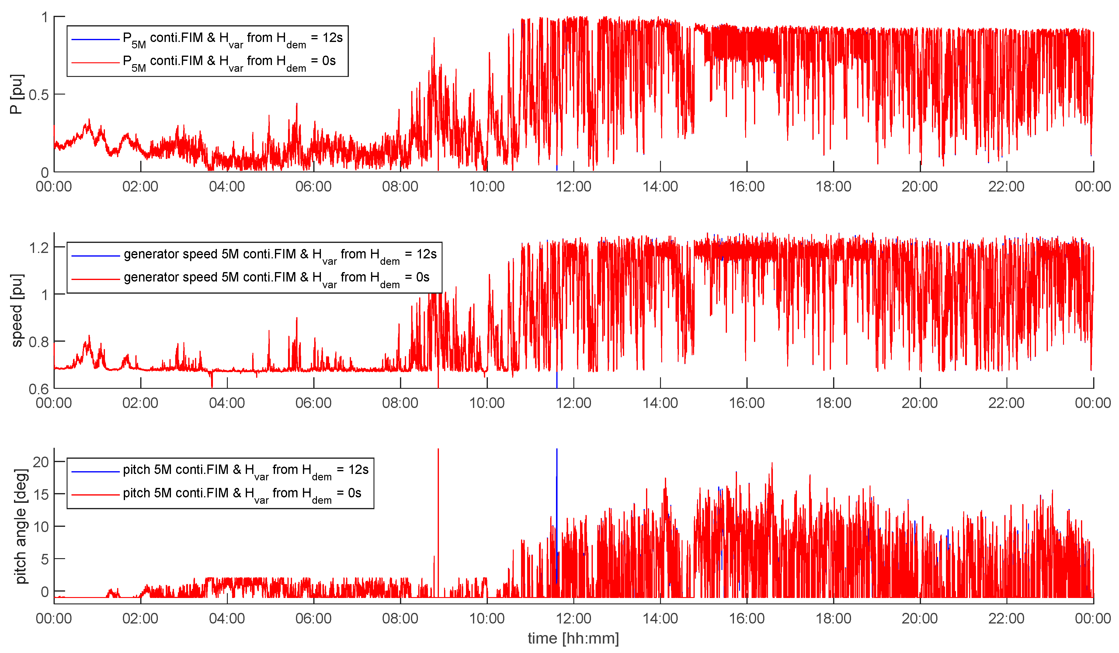
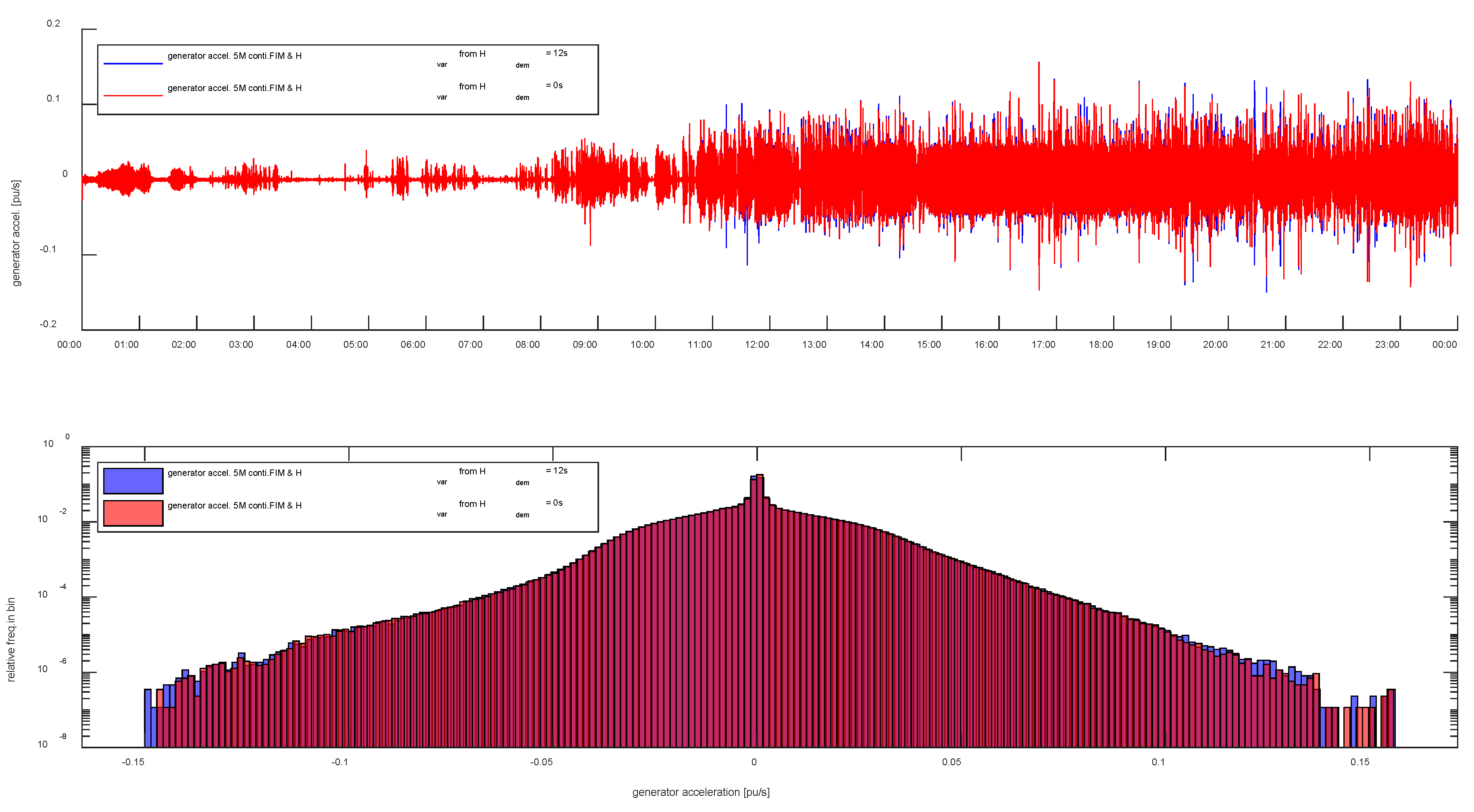
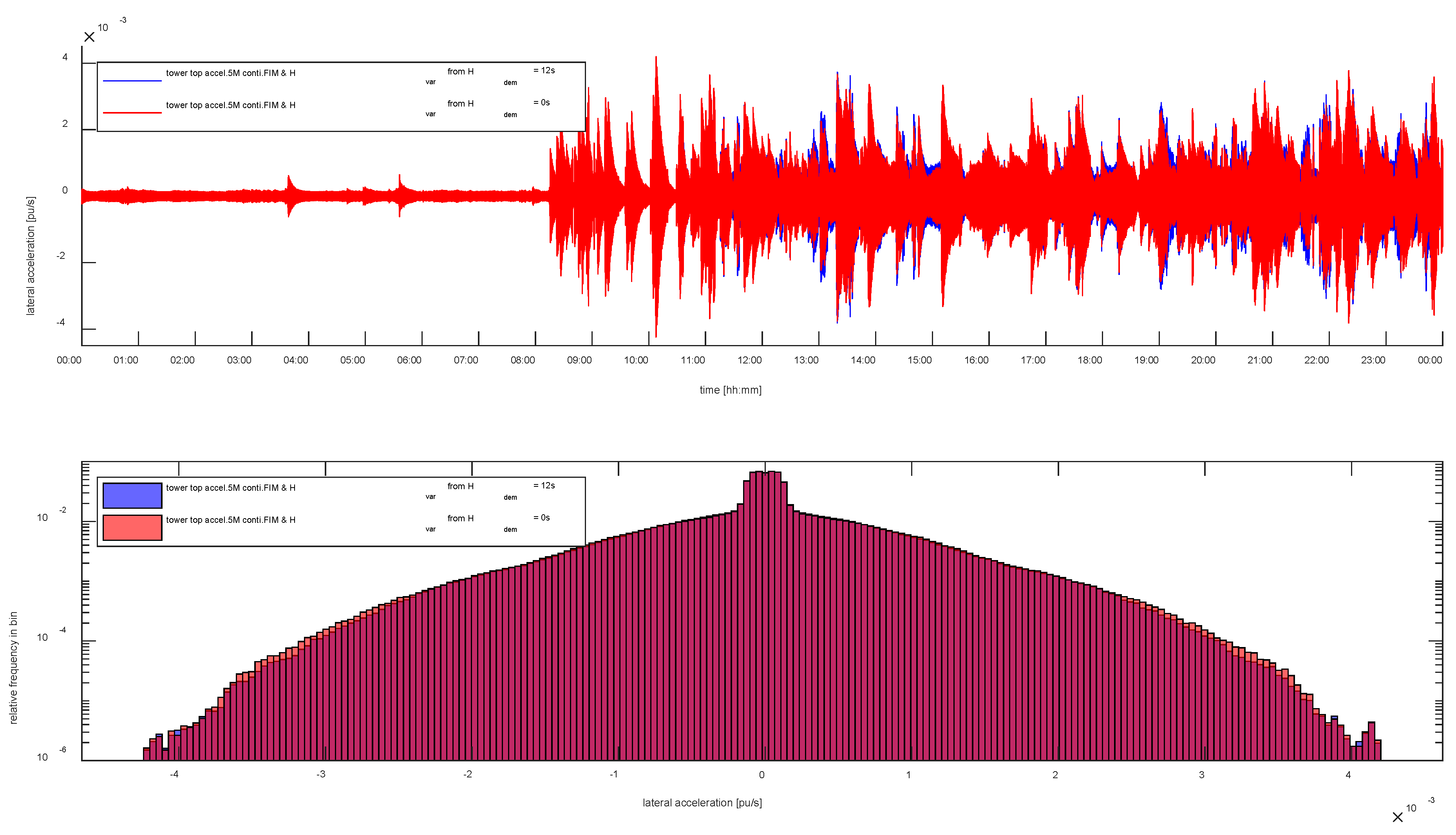
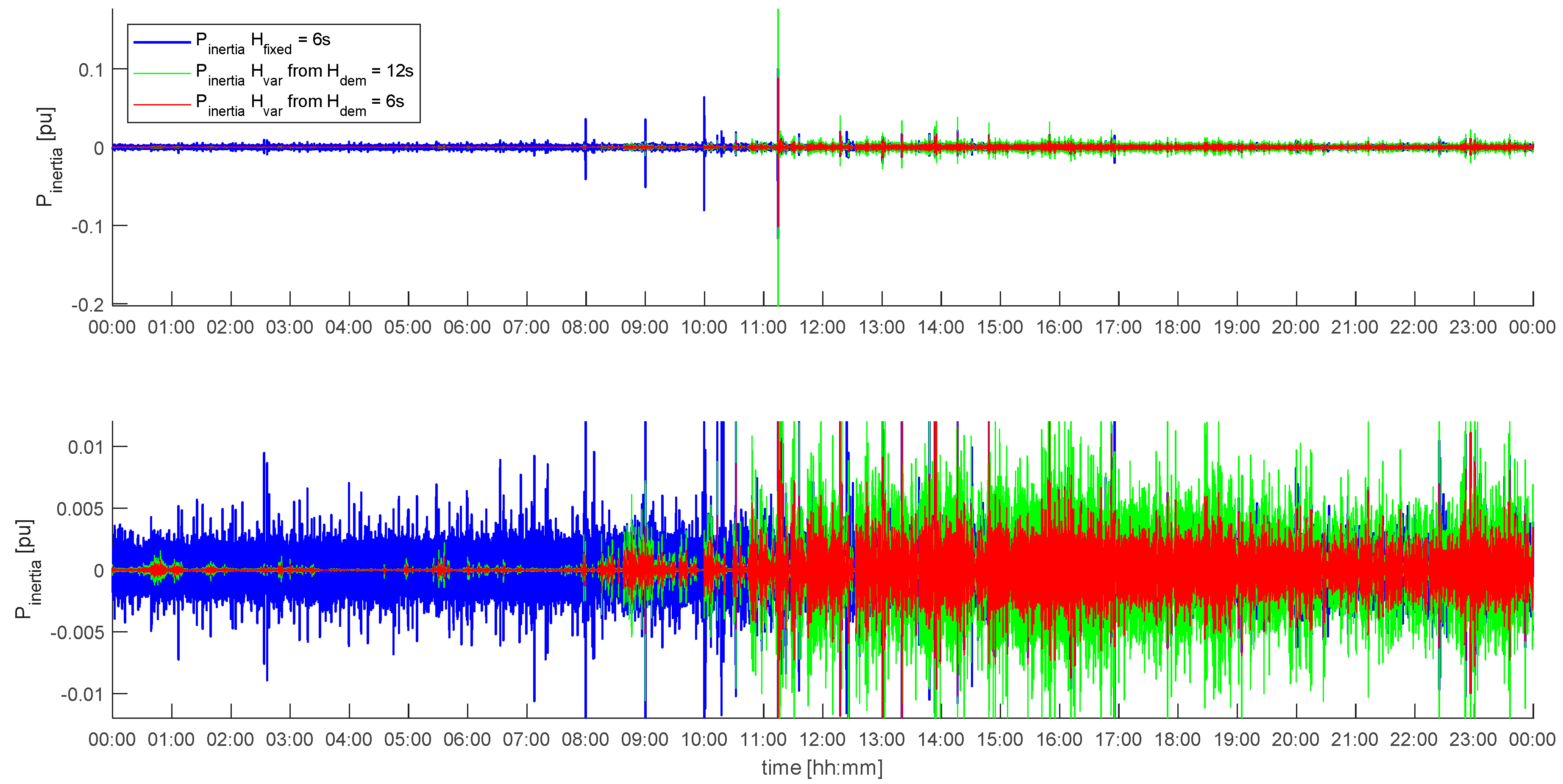
5.2. Effect of Variable H Controller on the WT

The effect that continuous FIM has on the WT was assessed in previous publications [5,29]. Therefore, only the additional effect that continuous inertia contribution with the H_var controller has on the WT shall be discussed here.

Different H_dem values are tested. Generally, the H_var controller causes little impact on the WT, which is already visible from the fact that the two curves in Figure 11 hardly differ. Since the continental European grid frequency only rarely exhibits large ROCOFs, H_dem is set to 12 s to achieve high power setpoint changes due to inertial response. This way, also the circumstances in smaller, i.e., more agile grids can be emulated. The analysis of all WT signals reveals that the acceleration of the generator and of the tower in lateral direction are affected most. Hence, these are the only signals considered here. However, Figure 14 and Figure 15 show that even H_dem = 12 s has hardly any effect on the generator acceleration and on the lateral tower acceleration, respectively. It has to be mentioned, that the grid frequency recorded on 5 April 2017 is representative of a normal day in continental Europe. Although it did not contain any extreme events, it is still challenging in terms of inertial response, as the grid frequency appears to vary with extreme ROCOFs due to electromagnetic illusions.

These findings confirm the results yielded in a field test and fatigue load analysis conducted earlier. During a research project carried out with the WT manufacturer Suzlon Energy, a small multi-MW WT was equipped with the H_var controller where H_dem was set to 6 s. The f_grid time series were artificially generated to contain severe frequency events. With these time series the performance of the WT and the resulting loads were assessed at different wind speeds. The fatigue load analysis revealed that even with regularly occurring severe events in f_grid the H_var controller consumes only very little lifetime of the WT [9]. Also, as one consequence of the findings of this project, the demanded inertia constant is set to H_dem = 12 s here.

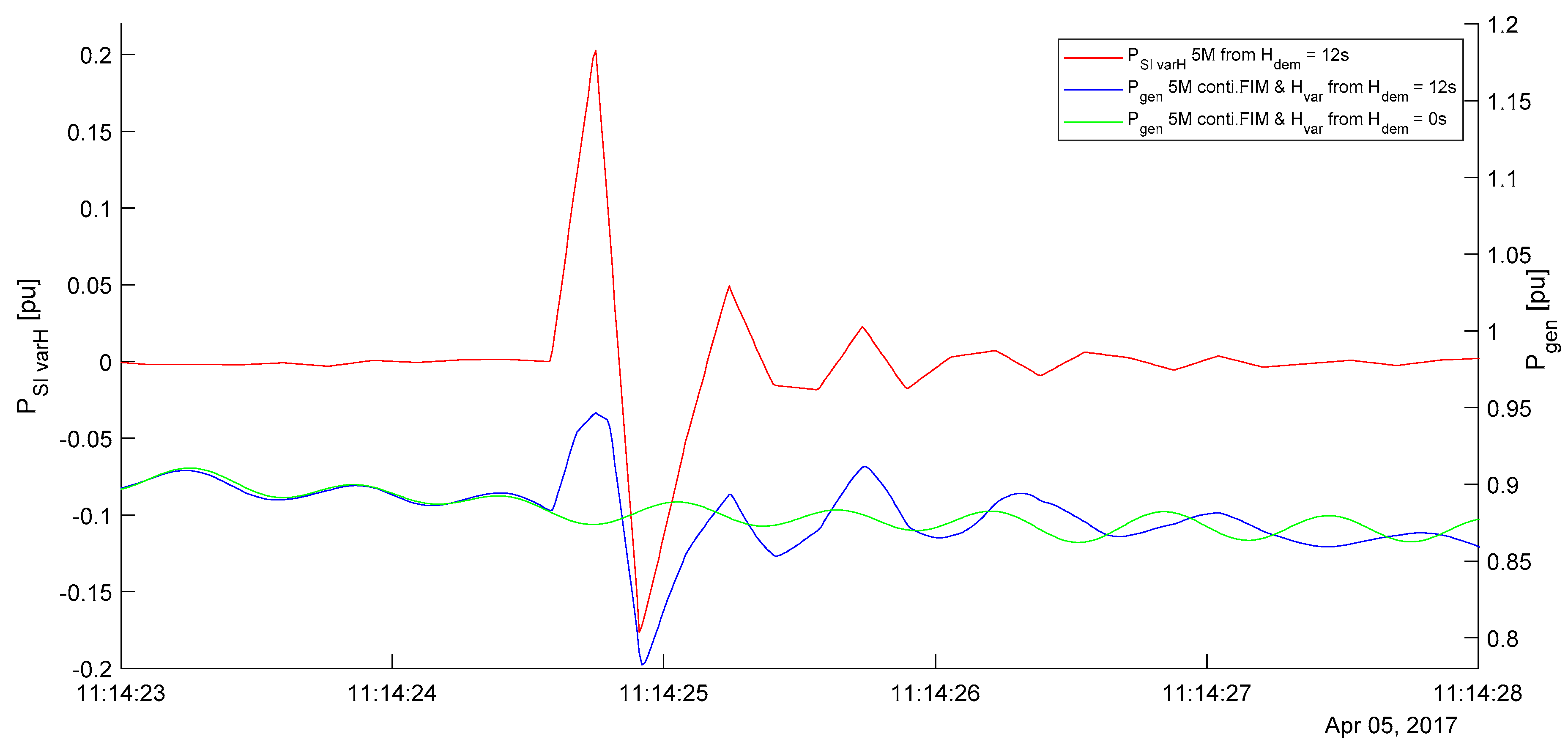
5.3. Effect of Continuous FIM and Inertia Provision on the Grid

The advantage of continuous FIM on the power infeed of the WT is published already [5]. It has to be added though, that such rapid optimization of the grid utilization is entirely inconceivable with conventional power plants (thermal or hydro) that are based on AC-connected generators. Hence, for their power to be reliably available for maintaining the balance between generation and demand (f_grid control), either oversized feeders or conservative power truncation is inevitable.

When a generator provides inertia to the grid, it produces power that is a function of the frequency, ω = 2∙π∙f_grid, and the ROCOF, see Equation (13).

$$P_{inertia}=J·\omega ·\frac{d\omega }{dt}$$

(13)

When a variable speed WT provides inertia to the grid, it is not the inherent inertia, J, which determines P_inertia. Instead, the frequency converter has to be controlled such that the WT exhibits inertial behaviour, i.e., it produces synthetic inertia. Hence, H_dem, or in case the H_var controller is applied, H_var is decisive for the inertial power, see Equation (14).

$$P_{inertia}=\frac{2·H_{var}·P_{rated}}{\omega }·\frac{d\omega }{dt}$$

(14)

This power theoretically contributes to the loading of the feeder that connects the WT with the grid. However, Figure 10 reveals that there is virtually no coupling between continuous FIM and inertial response, i.e., P_inertia. In addition, it has to be pointed out that the mean value of P_inertia is zero in normal power system operation (only if there is a persistent deviation of f_grid from its rated value the mean value of P_inertia ≠ 0). This is further shown in Figure 16 and Figure 17. Hence, P_inertia cannot interfere with the transformer temperature and it can only temporarily interfere with V_C.

The effect of inertia contribution on the grid can be quantified with the inertial energy, E_inertia. When considering certain durations, such as the 24 h of the 5 April 2017, the energy exchange between grid and WT, which results from inertia contribution, can be derived according to Equation (15).

$$E_{inertia}={{\displaystyle \int }}_{5/4/2017 00:00}^{5/4/2017 24:00}\left(\sqrt{P_{inertia}{\left(t\right)}^2}\right)dt$$

(15)

To assess the ability to contribute to system inertia, H_dem of the H_var controller in the 5M is set to 6 s and to 12 s. The resulting P_inertia are compared with the P_inertia of an AC connected synchronous generator with a fixed inertia constant H_fixed = 6 s. Figure 16 shows these three different P_inertia for the 24 h of 5 April 2017. Comparing Figure 16 with Figure 11 reveals that the inertia contribution of the 5M depends on the prevailing power operating point. Integrating P_inertia according to Equation (15) leads to the inertial energies, E_inertia, which are listed in

Table 1. E_inertia from an AC connected synchronous generator with H = 6 s, E_inertia from the 5M with H_var controller and H_dem = 6 s and H_dem = 12 s.

	5 April 2017 00:00–24:00	5 April 2017 00:00–12:00	5 April 2017 12:00–24:00
Hfixed = 6 s	88.2029 kWh	41.5384 kWh	46.6645 kWh
Hvar from Hdem = 6 s	33.0589 kWh	4.3307 kWh	28.7283 kWh
Hvar from Hdem = 12 s	66.1327 kWh	8.6603 kWh	57.4724 kWh

. In Table 1 E_inertia is not only given for the whole day, but also for the first half and for the second half of the day.

In the morning, when the wind speed is low, the inertia contribution is also low. From a grid point of view, this is no problem. In this case, either a larger number of WTs has to cover the consumption in the grid, or other generators have to produce the demanded power and, hence, also the necessary inertia.

In the afternoon, when the wind speed is high, the 5M has to deal with continuous FIM, but the inertia contribution increases nonetheless.

Table 1 shows very clearly that the inertia contribution of the 5M is comparable to that of a synchronous generator. When H_dem is set to 12 s, the inertia contribution in the afternoon of 5 April 2017 is even 23% greater than that of the synchronous generator. It has to be kept in mind that in the scenario simulated here, the 5M is burdened with continuous FIM. Hence, it operates only intermittently and only for short durations at rated power and rated speed. Each time the speed drops the inertia contribution drops as well, see Figure 5. Without FIM the inertia contribution could increase even further in the afternoon.

Table 1 further reveals that doubling H_dem leads to a doubling of E_inertia. This proves that inertia contribution has virtually no impact on the rotational speed and on the aerodynamic performance of the WT.

The discussion so far revolves around results that are produced from the power demand necessary for inertial response, i.e., P_{SI_varH} in Figure 6, as it is not possible to extract P_inertia from P_5M. There are several factors that make such a comparison impossible: P_inertia is camouflaged in P_5M by the turbulent wind and the motion of the mechanical components of the WT, namely the generator rotor, the blades in-plane and out-of-plane, as well as the motion of the tower in longitudinal and in lateral direction. The power reference for the frequency converter (in the model this variable is called P_setpoint, see Figure 3) is derived from the measured rotational speed of the generator. The driving power that is instantaneously available for the WT is determined by the wind speed and the aforementioned motions of mechanical components, as these interfere with the ambient wind speed, leading to a perceived wind speed. Therefore, P_inertia can be magnified or weakened in single occasions. Considering longer durations, these effects are assumed to level out. However, very rapid P_inertia variations cannot be realized by the generator–converter unit with its time constant (T_PT1_geno_substi = 25 ms). It has to be kept in mind, however, that the response of the AC-connected synchronous generator (in Table 1) is derived with Equation (14). The limited dynamic response of a synchronous generator is not taken into account here either.

Figure 17 shows an exemplified comparison between the power setpoint for inertial response, P_{SI_varH}, and the power that the 5M feeds into the grid, P_gen. To show a drastic example Figure 17 shows the response to the peak in ROCOF at 11:14 (compare Figure 2), which is assumed to be an electromagnetic illusion. Figure 17 reveals that P_gen follows P_{SI_varH} quite well (note that the ranges of the two y-axes in Figure 17 are identical). The difference in magnitude of the excursion in P_{SI_varH} and in P_gen is caused by the damping effects of the power controller and the generator–converter unit. Hence, the comparison in Table 1 is deemed valid.

The energy yield of the 5M is virtually not affected by inertial response. During the 24 h of 5 April 2017, the 5M generates 57,097.4 kWh without inertial response and 57,095.5 kWh with the H_var controller and H_dem = 12 s; both with continuous FIM.

6. Conclusions

This paper presents simulation results of continuous FIM and continuous provision of synthetic inertia with a WT. The case simulated is based on measurements. The conclusion of this study is that WTs can deal with excessively weak grid connections and, at the same time, can contribute to grid inertia continuously. With their rapid power control, WTs can adjust their power infeed to satisfy the needs of limited grid connection points a lot quicker than conventional power plants. By doing so, their power is available reliably with neither undue waste of energy nor overdimensioned grid enhancements. At the same time, they can contribute to grid inertia to a larger extent than conventional power plants. In the study at hand, the inertia constant reaches up to 12 s in rated operation of the WT. This number has to be put into perspective with the inertia constants of conventional power plants. These range from 2 s to 9 s [30], in case of hydro power plants only up to 4 s, and in the case of generators with two pole pairs up to 10 s [10]. Hence, WTs enhance angular stability in a power system to a larger extent than conventional power plants.

While many current grid codes focus on grid frequency support by WTs in prespecified events (fast frequency response), this study shows that it is advantageous when WTs provide inertia to the grid continuously with the H_var controller. By doing so, the grid reliably maintains controllability of the frequency. The WTs, on the other hand, suffer neither undue wear, nor noticeable loss of energy yield.

References

1. Bundesnetzagentur, Pressemitteilung: Bundesnetzagentur Veröffentlicht Zahlen zu Redispatch und Einspeisemanagement für 2017. 2018. Available online: https://www.bundesnetzagentur.de/SharedDocs/Downloads/DE/Allgemeines/Presse/Pressemitteilungen/2018/20180618_NetzSystemSicherheit.pdf?__blob=publicationFile&v=2 (accessed on 1 May 2019).
2. Ministerium für Energiewende, Landwirtschaft, Umwelt, Natur und Digitalisierung (MELUND) Schleswig-Holstein, Kurzbericht zum Engpassmanagement in Schleswig-Holstein. 2018. Available online: https://www.schleswig-holstein.de/DE/Fachinhalte/E/erneuerbareenergien/Bericht_Einspeisemanagement.pdf;jsessionid=CAD6BCDD96E9F0CFFB6472B2DA2B6E5F?__blob=publicationFile&v=1 (accessed on 1 May 2019).
3. Larscheid, P.; Maercks, M.; Dierkes, S.; Moser, A.; Patzack, S.; Vennegeerts, H.; Rolink, J.; Wieben, E. Increasing the Hosting Capacity of RES in Distribution Grids by Active Power Control. In Proceedings of the International ETG Congress, Bonn, Germany, 17–18 November 2015; Available online: https://ieeexplore.ieee.org/stamp/stamp.jsp?tp=&arnumber=7388485&tag=1 (accessed on 1 May 2019).
4. Jauch, C. FH Flensburg erforscht dynamische Leistungsbereitstellung durch WEA. Ingenieurspiegel 2013, 4, 20–21. [Google Scholar]
5. Jauch, C.; Gloe, A.; Hippel, S.; Thiesen, H. Increased Wind Energy Yield and Grid Utilisation with Continuous Feed-In Management. Energies 2017, 10, 870. [Google Scholar] [CrossRef]
6. Jauch, C.; Gloe, A. Improved feed-in management with wind turbines. In Proceedings of the 15th Wind Integration Workshop, Vienna, Austria, 15–17 November 2016; Available online: https://www.researchgate.net/publication/311485049_Improved_Feed-in_Management_with_Wind_Turbines (accessed on 31 May 2019).
7. Eriksson, R.; Modig, N.; Elkington, K. Synthetic inertia versus fast frequency response: A definition. IET Renew. Power Gener. 2018, 12, 507–514. [Google Scholar] [CrossRef]
8. Fleming, P.A.; Aho, J.; Buckspan, A.; Ela, E.; Zhang, Y.; Gevorgian, V.; Scholbrock, A.; Pao, L.; Damiani, R. Effects of power reserve control on wind turbine structural loading. Wind Energy 2015, 19, 453–469. [Google Scholar] [CrossRef]
9. Gloe, A.; Jauch, C.; Thiesen, H.; Viebeg, J. Inertial Response Controller Design for a Variable Speed Wind Turbine. WETI Flensbg. Univ. Appl. Sci. 2018. [Google Scholar] [CrossRef]
10. Kundur, P. Power System Stability and Control; McGraw-Hill: New York, NY, USA, 1994. [Google Scholar]
11. Bird, L.; Lew, D.; Milligan, M.; Carlini, E.M.; Estanqueiro, A.; Flynn, D.; Gomez-Lazaro, E.; Holttinen, H.; Menemenlis, N.; Orths, A.; et al. Wind and solar energy curtailment: A review of international experience. Renew. Sustain. Energy Rev. 2016, 65, 577–586. [Google Scholar] [CrossRef] [Green Version]
12. Ulbig, A.; Borsche, T.S.; Andersson, G. Impact of low rotational inertia on power system stability and operation. In Proceedings of the 19thWorld Congress of the International Federation of Automatic Control (IFAC 2014), Capetown, South Africa, 24–29 August 2014; Available online: https://reader.elsevier.com/reader/sd/pii/S1474667016427618?token=1130DA98E61ECBD9185907D2DE5A4F90E659BFC754B1D06E7CABAF20EF66856E7A2E7072C5268A2049CBF7AD6D84C5A0 (accessed on 3 May 2019).
13. Tielens, P.; Hertem, D.V. The relevance of inertia in power systems. Renew. Sustain. Energy Rev. 2016, 55, 999–1009. Available online: http://www.sciencedirect.com/science/article/pii/S136403211501268X (accessed on 3 May 2019).
14. Gonzalez-Longatt, F.M. Activation schemes of synthetic inertia controller on full converter wind turbine (type4). In Proceedings of the IEEE Power and Energy Society General Meeting, Denver, CO, USA, 26–30 July 2015; Available online: https://ieeexplore.ieee.org/stamp/stamp.jsp?tp=&arnumber=7286430 (accessed on 2 May 2019).
15. EirGrid; Soni, All Island TSO Facilitation of Renewables Studies. 2010. Available online: http://www.eirgridgroup.com/site-files/library/EirGrid/Facilitation-of-Renewables-Report.pdf (accessed on 2 May 2019).
16. Hydro Québec TransÉnergie. Technical Requirements for the Connection of Generation Facilities to the Hydro-Québec Transmission System. Supplementary Requirements for Wind Generation. 2005. Available online: http://www.hydroquebec.com/transenergie/fr/commerce/pdf/eolienne_transport_en.pdf (accessed on 2 May 2019).
17. Red Electrica. Technical Requirement for Wind Power and Photovoltaic Installations and Any Generating Facilities Whose Technology Does Not Consist on a Synchronous Generator Directly Connected to the Grid. Available online: http://joaocarvalhosa.weebly.com/uploads/6/6/1/5/6615139/espanha.pdff (accessed on 3 May 2019).
18. Salehi Dobakhshari, A.; Azizi, S.; Ranjbar, A.M. Control of Microgrids: Aspects and Prospects. In Proceedings of the IEEE International Conference on Networking, Sensing and Control, Delft, The Netherlands, 11–13 April 2011; Available online: https://ieeexplore.ieee.org/stamp/stamp.jsp?tp=&arnumber=5874892 (accessed on 2 May 2019).
19. Gloe, A.; Jauch, C.; Craciun, B.; Winkelmann, J. Continuous provision of synthetic inertia with wind turbines: Implications for the wind turbine and for the grid. IET Renew. Power Gener. 2019, 13, 668–675. [Google Scholar] [CrossRef]
20. Jonkman, J.; Butterfield, S.; Musial, W.; Scott, G. Definition of a 5-MW Reference Wind Turbine for Offshore System Development. Available online: http://pop.h-cdn.co/assets/cm/15/06/54d150362c903_-_38060.pdf (accessed on 3 May 2019).
21. Jauch, C. First Eigenmode Simulation Model of a Wind Turbine—for Control Algorithm Design. WETI Flensbg. Univ. Appl. Sci. 2016. Available online: https://www.researchgate.net/publication/312935476_First_Eigenmode_Simulation_Model_of_a_Wind_Turbine_-_for_Control_Algorithm_Design (accessed on 3 May 2019). [CrossRef]
22. Gloe, A.; Thiesen, H.; Jauch, C. Grid frequency analysis for assessing the stress on wind turbines. In Proceedings of the 15th Wind Integration Workshop, Vienna, Austria, 15–17 November 2016; Available online: https://www.researchgate.net/publication/311485049_Improved_Feed-in_Management_with_Wind_Turbines (accessed on 3 May 2019).
23. Thiesen, H.; Jauch, C. Identifying electromagnetic illusions in grid frequency measurements for synthetic inertia provision. In Proceedings of the IEEE CPE-POWERENG 2019, 13th International Conference on Compatibility, Power Electronics and Power Engineering, Sonderborg, Denmark, 23–25 April 2019. [Google Scholar]
24. Hafiz, F.; Abdennour, A. An adaptive neuro-fuzzy inertia controller for variable-speed wind turbines. Renew. Energy 2016, 92, 136–146. [Google Scholar] [CrossRef]
25. Andresen, M. Simulation eines Einspeisereglers für Erzeugungsanlagen. Bachelor‘s Thesis, WSTECH GmbH, Flensburg, Germany, 2 January 2019. [Google Scholar]
26. MATLAB Version: 9.4.0.813654 (R2018a). Available online: http://uk.mathworks.com/products/matlab/ (accessed on 2 May 2019).
27. Jonkman, J.M.; Jonkman, B.J. FAST modularization framework for wind turbine simulation: Full-system linearization. In Proceedings of the Conference: Science of Making Torque from Wind (TORQUE 2016), Munich, Germany, 5–7 October 2016; Available online: https://www.nrel.gov/docs/fy17osti/67015.pdf (accessed on 3 May 2019).
28. Nise, N.S. Control Systems Engineering, 3rd ed.; John Wiley & Sons: Hoboken, NJ, USA, 2000; ISSN/ISBN 0-471-36601-3. [Google Scholar]
29. Jauch, C.; Gloe, A. Flexible Wind Power Control for Optimal Power System Utilisation. In Proceedings of the WindAc Africa 2017, Cape Town, South Africa, 14–15 November 2017; Available online: https://www.researchgate.net/publication/321212504_Flexible_Wind_Power_Control_For_Optimal_Power_System_Utilisation (accessed on 3 May 2019).
30. Stevenson, W.; Grainger, J. Power System Analysis; McGraw-Hill: New York, NY, USA, 1994. [Google Scholar]
Figure 1. Setup of the case study of Flensburg campus supplemented by a 5 MW WT (5M) with connection to the external grid.
Energies 12 03013 g001
Figure 2. Measured grid frequency and ROCOF (top); frequency spectrum of grid frequency (bottom).
Energies 12 03013 g002
Figure 3. Close loop power control in the 1st eigenmodes model of a WT.
Energies 12 03013 g003
Figure 4. Bode plots of the open power control loop.
Energies 12 03013 g004
Figure 5. Variable inertia constant, Hvar, for the demanded rated inertia constants Hdem = 6 s and Hdem = 12 s. Constant inertia constant H = 6 s.
Energies 12 03013 g005
Figure 6. Control circuit for continuous FIM and inertial response with Hvar controller.
Energies 12 03013 g006
Figure 7. P vs. speed characteristic and linearization around the operating point.
Energies 12 03013 g007
Figure 8. WT drive train model.
Energies 12 03013 g008
Figure 9. Block diagram of WT system from P_ref to speed_gen.
Energies 12 03013 g009
Figure 10. Bode plots of the transfer functions GWT(s), GPI_P_dem(s) and GTR(s) (top) in comparison to the frequency spectra of the different excitations: ROCOF, PC and QC (bottom).
Energies 12 03013 g010
Figure 11. WT power (top) generator speed (middle) and pitch angle (bottom) of 5M for the case of continuous FIM operation (red curves) and for the case of continuous FIM with inertial response (blue curves in the background).
Energies 12 03013 g011
Figure 12. Generator acceleration (top) and frequency distribution of generator acceleration (bottom) of 5M in continuous FIM operation for two different generator-converter time constants.
Energies 12 03013 g012
Figure 13. Lateral tower top acceleration (top) and frequency distribution of lateral tower top acceleration (bottom) of 5M in continuous FIM operation for two different generator–converter time constants.
Energies 12 03013 g013
Figure 14. Generator acceleration (top) and frequency distribution of generator acceleration (bottom) of 5M when performing continuous FIM, with and without continuous inertia provision.
Energies 12 03013 g014
Figure 15. Lateral tower top acceleration (top) and frequency distribution of lateral tower top acceleration (bottom) of 5M when performing continuous FIM, with and without continuous inertia provision.
Energies 12 03013 g015
Figure 16. Pinertia from an AC connected synchronous generator with H = 6 s (blue), Pinertia from the 5M with Hvar controller and Hdem = 6 s (red) and Hdem = 12 s (green). The bottom diagram is a zoom-in view of the top diagram.
Energies 12 03013 g016
Figure 17. The inertial response power setpoint, PSI_var, (red) and the generator power, Pgen, from the 5M. Pgen is shown for the case of FIM only (green) and FIM with inertial response (blue).
Energies 12 03013 g017