Atomic Scheduling of Appliance Energy Consumption in Residential Smart Grids

Abstract

Most of the current formulations of the optimal scheduling of appliance energy consumption use the vectors of appliances’ scheduled energy consumption over equally divided time slots of a day as optimization variables, which does not take into account the atomicity of certain appliances’ operations, i.e., the non-interruptibility of appliances’ operations and the non-throttleability of the energy consumption patterns specific to their operations. In this paper, we provide a new formulation of atomic scheduling of energy consumption based on the optimal routing framework; the flow configurations of users over multiple paths between the common source and destination nodes of a ring network are used as optimization variables, which indicate the starting times of scheduled energy consumption, and optimal scheduling problems are now formulated in terms of the user flow configurations. Because the atomic optimal scheduling results in a Boolean-convex problem for a convex objective function, we propose a successive convex relaxation technique for efficient calculation of an approximate solution, where we iteratively drop fractional-valued elements and apply convex relaxation to the resulting problem until we find a feasible suboptimal solution. Numerical results for the cost and peak-to-average ratio minimization problems demonstrate that the successive convex relaxation technique can provide solutions close to and often identical to global optimal solutions.

1. Introduction

We study the problem of scheduling electrical appliance energy consumption in residential smart grids. Our goal in revisiting this well-known problem of energy consumption scheduling (e.g., References [1,2,3,4,5,6,7,8,9,10,11,12,13]) is to establish a new formulation of optimal scheduling problems where we take into account the atomicity of operations by household appliances and to provide efficient solution techniques for the formulated optimal scheduling problems. By atomicity, we mean the non-interruptibility of appliances’ operations and the non-throttleability of the energy consumption patterns specific to their operations. As we will show later, the atomicity—the load characteristic newly introduced in this work—generalizes the characteristics of non-interruptibility and non-throttleability by allowing a prescribed usage pattern, which can vary over time from the beginning to the end of its operation with possible gaps in between.

Note that the scheduling of electrical appliance energy consumption is a key to the autonomous demand-side management (DSM) for residential smart grids in optimizing energy production and consumption; the scheduling is based on smart meters installed at users’ premises and the two-way digital communications between a utility company and users through the smart meters, and the typical goals of DSM include consumption reducing and shifting, which lead into lower peak-to-average ratio (PAR) and energy cost [14].

Since the energy consumption scheduling was formulated as an optimization problem using energy consumption scheduling vectors as optimization variables representing appliances’ scheduled hourly energy consumption over a day [2], there have been published a number of papers on the subjects of appliance energy consumption scheduling and related billing/pricing mechanisms based on this formulation. For instance, the issue of optimality and fairness in autonomous DSM is studied in relation with billing mechanisms in References [7], while the same issue is studied but in the context of user privacy in Reference [10]. The cost and PAR minimization problems, which are separately formulated in Reference [2], are integrated into a PAR-constrained cost minimization problem in Reference [12]. This integration is also further extended to take into account consumers’ preference on operation delay and power gap using multiple objective functions. In Reference [13], instead of typical concave n-person games, the Rubinstein–Stahl bargaining game model is used to capture the interaction between the supplier and the consumers through a retail price vector in lowering PAR to a certain desired value.

In most existing works on the energy consumption scheduling for autonomous DSM in smart grid, however, no serious attention has been given to the microstructure of scheduled energy consumption over time slots; their major focus is on the optimal value of an objective function that is only based on the aggregate load from the scheduled energy consumption. Few exceptions in this regard include the works on the integration of consumers’ preference [12] and the use of load consumption curves in the objective function [4] and scheduling of noninterruptible tasks with price uncertainty [8] and load uncertainty [3]. None of them, however, can guarantee both the non-interruptibility of the operations and the non-throttleability of the energy consumption patterns, the latter of which are generally not constant over time and specific to appliances’ operations [15,16,17].

Below are some scenarios illustrating the importance of the atomicity of appliance operations.

• When a user washes clothes, the washing machine should be continuously on for a certain period depending on the amount of laundry, e.g., for two hours, during which the operation of the clothes washer cannot be interrupted and the supplied power cannot be reduced arbitrarily. As the washing task can be activated anytime within a specified period, e.g., from 9 a.m. to 3 p.m. when the user is out to work, the major goal of autonomous DSM is to determine the optimal two-hour time slot to complete the task when the energy price is lowest during the specified period.
• For heavier-duty tasks like charging the battery of a plug-in hybrid electric vehicle (PHEV), again, the continuity of the operation is important, e.g., four hours of uninterruptible charging to maintain the lifetime of PHEV’s battery.
• Appliances such as a rice cooker can significantly contribute to the overall cost saving if handled properly. Some rice cookers’ function may take more than one hour for completion, e.g., the slow cooking function for delicate soup, whereby the cooking process can be scheduled within any time-shot during the day.

Considering that most of the operations subject to DSM are either atomic as such (e.g., laundry cleaning by a clothes washer) or consist of atomic suboperations (e.g., house heating by a heater operating in the morning and in the evening) [11], we provide a new formulation of the optimization problem for atomic scheduling of appliance energy consumption and efficient solution techniques for the resulting problems in this paper. Atomic scheduling has been mostly discussed in the context of concurrent task scheduling on a multiprocessor/core system on a chip (SOC) [18] or transaction processing [19]. To the best of our knowledge, our work is the first attempt to formulate atomic scheduling of appliance energy consumption in the autonomous DSM for residential smart grid, where both the non-interruptibility of appliances’ operations and the non-throttleability of the energy consumption patterns are taken into account and guaranteed.

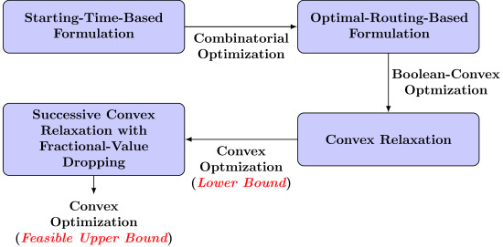
The rest of the paper is organized as follows: In Section 2, we review and discuss the issues of the current formulation of appliance energy consumption scheduling based on energy consumption scheduling vectors defined over time slots. In Section 3, we describe a new formulation of the appliance energy consumption scheduling based on the optimal routing framework, which guarantees the atomicity of appliance operations, and a successive convex relaxation technique for the efficient solution of the Boolean-convex problem resulting from the new formulation for a given convex objective function. In Section 4, we demonstrate the performance of successive convex relaxation techniques through numerical results for the cost and PAR minimization problems. Section 5 concludes our work and discusses topics for further study.

2. Review of Current Formulation of Appliance Energy Consumption Scheduling

We first review the current formulation of the appliance energy consumption scheduling problem by formally describing it. The formulation described here is largely based on Reference [2] but with some modifications and extensions for clarity and better handling of scheduling intervals over a day boundary. Many notations and definitions in this section are applicable to the formulation of atomic scheduling problems in Section 3 as well.

Let $\mathcal{N}\triangleq \left\{1,\dots ,N\right\}$ denote a set of users in a residential smart grid whose appliances share a common energy source and are subject to autonomous DSM. Without loss of generality and for the ease of presentation, we assume that each user has only one appliance throughout the paper as in Reference [10]. (We use the term “user” and “appliance” interchangeably). In this case, a daily energy consumption scheduling vector of user n is defined as

$${\mathbf{x}}_n\triangleq \left[x_n^0,\dots ,x_n^h,\dots ,x_n^{H-1}\right]$$

(1)

where a scalar element $x_n^h$ denotes the energy consumption scheduled for a time slot $h\in \mathcal{H}\triangleq \left\{0,\dots ,H-1\right\}$. (Time slot numbering in this paper starts from 0, which makes it easier to handle energy consumption scheduling wrapping around the day boundary (i.e., from 11 p.m. to 6 a.m.) using modulo operation. See Equations (2) and (3) for details). A feasible energy consumption scheduling set for user n is given by

$$\begin{array}{cc}\hfill {\mathcal{X}}_n=& \left\{{\mathbf{x}}_n\right|\sum _{h\in {\mathcal{H}}_n}{x}_n^h=E_n,\hfill \\ \hfill & {\gamma }_n^{min}\le x_n^h\le {\gamma }_n^{max}, \forall h\in {\mathcal{H}}_n, x_n^h=0, \forall h\in \mathcal{H}\backslash {\mathcal{H}}_n\}\hfill \end{array}$$

(2)

where ${\gamma }_n^{min}$ and ${\gamma }_n^{max}$ are the minimum and the maximum energy levels for a time slot, $E_n$ is the total daily energy consumption of user n’s appliance, $\mathcal{H}\backslash {\mathcal{H}}_n$ is the relative complement of ${\mathcal{H}}_n$ in $\mathcal{H}$ (i.e., the set difference of $\mathcal{H}$ and ${\mathcal{H}}_n$), and ${\mathcal{H}}_n$ is a scheduling interval defined as follows:

$${\mathcal{H}}_n\triangleq \left\{h|h=i \mathrm{mod} H, \forall i\in \left[{\alpha }_n, {\beta }_n\right]\right\}$$

(3)

with ${\alpha }_n\in [0, H-1]$, ${\beta }_n\in [1, 2H-2]$, and $1\le {\beta }_n-{\alpha }_n\le H-1$.

With these definitions of scheduling vectors and feasible sets, the optimal scheduling is formulated as an optimization problem for a given objective function (e.g., total energy cost or PAR) as follows:

$$\underset{{\mathbf{x}}_n\in {\mathcal{X}}_n, \forall n\in \mathcal{N}}{\mathbf{minimize}} \psi \left(\mathbf{x}\right)$$

(4)

where

$$\mathbf{x}\triangleq \left[{\mathbf{x}}_1,\dots ,{\mathbf{x}}_N\right].$$

(5)

As shown in Reference [2], it is better to develop a DSM approach that optimizes the properties of the aggregate load of the users rather than individual user’s consumption. In fact, the optimal scheduling problems are formulated in terms of the total load across all users at each time slot h in Reference [2], i.e.,

$$L_h\left(\mathbf{x}\right)\triangleq \sum _{n\in \mathcal{N}}{x}_n^h.$$

(6)

Therefore, Equation (4) can be expressed as

$$\underset{{\mathbf{x}}_n\in {\mathcal{X}}_n, \forall n\in \mathcal{N}}{\mathbf{minimize}} \varphi \left(\mathit{L}\left(\mathbf{x}\right)\right)$$

(7)

where

$$\mathit{L}\left(\mathbf{x}\right)\triangleq \left[L_0\left(\mathbf{x}\right),\dots ,L_{H-1}\left(\mathbf{x}\right)\right].$$

(8)

Note that the objective function becomes

$$\varphi \left(\mathit{L}\left(\mathbf{x}\right)\right)=\sum _{h\in \mathcal{H}}{C}_h\left(L_h\left(\mathbf{x}\right)\right)$$

(9)

for the energy cost minimization problem, where $C_h(·)$ is a cost function indicating the cost of generating or distributing electricity energy by the energy source at a time slot h and

$$\varphi \left(\mathit{L}\left(\mathbf{x}\right)\right)=\frac{{\displaystyle H\underset{h\in \mathcal{H}}{max}{L}_h\left(\mathbf{x}\right)}}{{\displaystyle \sum _{n\in \mathcal{N}}{E}_n}}$$

(10)

for the PAR minimization problem.

A major issue with the formulation of optimal scheduling problems based on the energy consumption scheduling vectors in Equation (1) is that it cannot guarantee the atomicity of appliance operations, which is illustrated in Figure 1a. When a load from other appliances falls in the middle of the scheduling interval, especially that of non-shiftable appliances, the scheduled appliance energy consumption spreads over non-contiguous time slots, resulting in several gaps. Relatedly, the scheduled energy consumption may not provide enough power for appliances to carry out required operations because, during the scheduling, the energy levels over time slots are determined to achieve the optimal solution for the given objective function but not to meet the actual energy consumption requirements of the appliances for the operations. The atomic scheduling that will be described in Section 3, on the other hand, assigns contiguous time slots with a predefined pattern of operating energy levels (i.e., ${\gamma }_n^{op}(·)$) as shown in Figure 1b, even at the expense of increased penalty in optimization.

3. Atomic Scheduling of Appliance Energy Consumption

We assume that all appliance operations are atomic (i.e., no gaps in energy consumption during the operations) and that the operation of the appliance of user n requires ${\delta }_n$ contiguous time slots belonging to a scheduling interval of ${\mathcal{H}}_n$ with a predefined pattern of operating energy levels ${\gamma }_n^{op}\left(h\right)$—which become power levels when the time slot duration is an hour (i.e., $H=24$)—such that ${\gamma }_n^{op}\left(h\right)>{\gamma }_n^{min} \forall h\in [0, {\delta }_n-1]$ and ${\gamma }_n^{op}\left(h\right)={\gamma }_n^{min}$ otherwise. Clearly, ${\beta }_n\ge {\alpha }_n+{\delta }_n-1$. Without loss of generality, we set ${\gamma }_n^{min}$ to 0; the resulting daily energy consumption $E_n$, therefore, is given by

$$E_n=\sum _{h=0}^{{\delta }_n-1}{\gamma }_n^{op}\left(h\right).$$

(11)

Figure 2 shows an example of operating energy levels. Note that, if an appliance requires multiple, separate scheduling intervals (e.g., one for 6 a.m.–11 a.m. and the other for 1 p.m.–5 p.m.), it can be modeled as multiple (virtual) appliances, each of them having only one contiguous scheduling interval (i.e., appliance 1 with 6 a.m.–11 a.m. and appliance 2 with 1 p.m.–5 p.m.).

A simple and straightforward formulation of atomic scheduling is using the starting times of operations as optimization variables, i.e.,

$$\mathbf{s}\triangleq \left[s_1,\dots ,s_N\right]$$

(12)

where a feasible set of starting times for user n is given by

$${\mathcal{S}}_n\triangleq \left\{s_n|s_n=i \mathrm{mod} H, \forall i\in [{\alpha }_n, {\beta }_n-{\delta }_n+1]\right\}$$

(13)

The total load across all users at each time slot h, therefore, can be expressed in terms of starting times $s_n\in {\mathcal{S}}_n, \forall n\in \mathcal{N}$, as follows:

$$L_h\left(\mathbf{s}\right)\triangleq \sum _{n\in \mathcal{N}}{\gamma }_n^{op}\left(\left(h-s_n\right) \mathrm{mod} H\right)I_{{\mathcal{R}}_n\left(s_n\right)}\left(h\right)$$

(14)

where ${\mathcal{R}}_n\left(s_n\right)$ is a range of user n’s appliance operation for $s_n$ defined by

$${\mathcal{R}}_n\left(s_n\right)\triangleq \left\{h|h=i \mathrm{mod} H, \forall i\in \left[s_n, s_n+{\delta }_n-1\right]\right\}$$

(15)

and $I_{{\mathcal{R}}_n\left(s_n\right)}\left(h\right)$ is an indicator function; note that, for a set $\mathcal{A}$, the indicator function is defined as

$$I_{\mathcal{A}}\left(a\right)\triangleq \left\{\begin{array}{cc}1\hfill & \mathrm{i}\mathrm{f} a\in \mathcal{A},\hfill \\ 0\hfill & \mathrm{o}\mathrm{t}\mathrm{h}\mathrm{e}\mathrm{r}\mathrm{w}\mathrm{i}\mathrm{s}\mathrm{e}.\hfill \end{array}\right.$$

(16)

Because the feasible set is now discrete, we have to evaluate the objective function for all the elements in the feasible set, which makes the optimization problem impractical for large N and H. For instance, when N = 100 and H = 24 with the worst case scenario of ${\alpha }_n$ = 0, ${\beta }_n$ = 23, and ${\delta }_n$ = 1 for all $n\in \mathcal{N}$, global optimization by direct enumeration would require evaluation of the objective function ${24}^{100}$ times, which is on the order of ${10}^{138}$ times. To address the scalability issue, therefore, we provide an alternative formulation of atomic scheduling based on the optimal routing framework, which is amenable to convex relaxation and enables systematic analysis of suboptimal solutions with upper and lower bounds.

3.1. Optimal Routing-Based Formulation

We provide a new formulation of the optimal scheduling of appliance energy consumption based on the framework of optimal routing in networking [20]; this new formulation takes into account the atomicity of appliance operations in scheduling without taking any additional objective functions.

As for optimization variables, instead of the energy consumption scheduling vector ${\mathbf{x}}_n$ in (1), we use flow configurations of users over multiple paths between the common source and destination nodes of the network shown in Figure 3a (this is for the case of hourly time slots, i.e., H = 24), which are defined as follows:

The users belonging to the set $\mathcal{N}$ share a set $\mathcal{P}$ of paths connecting the source node $\mathbf{S}$ and the destination node $\mathbf{D}$, where the path set $\mathcal{P}$ is defined as

$$\mathcal{P}\triangleq \left\{p^{i,j}|i=0,\dots ,H-1, j=1,\dots ,H-1\right\}$$

(17)

where i and j are the starting node number on the ring of a path and the number of hops, respectively; for instance, as illustrated in Figure 3a, $p^{9,3}$ is a three-hop path consisting of links $l^{9,10}$, $l^{10,11}$, and $l^{11,12}$ on the ring. Note that we do not take into account the radial links connecting the source and the destination nodes to and from the intermediate nodes on the ring in calculating hop counts and path/link costs. (This means that their link costs are zero). We now define $f_n^s$ as a flow that user n sends on path $p^{s,{\delta }_n}$, which represents an atomic operation of user n’s appliance with starting time slot s and duration of ${\delta }_n$ slots. Figure 3b shows the mapping of all possible atomic appliance operations of two users (i.e., ${\alpha }_1$ = 0, ${\beta }_1$ = 5, ${\delta }_1$ = 2 for user 1 and ${\alpha }_2$ = 9, ${\beta }_2$ = 14, ${\delta }_2$ = 3 for user 2) into corresponding groups of flows (i.e., $f_1^0,\dots ,f_1^4$ for user 1 and $f_2^9,\dots ,f_2^{12}$ for user 2).

We use the flow configurations of all users as the optimization variables, which are defined as follows:

$$\mathbf{f}\triangleq \left[{\mathit{f}}_1,\dots ,{\mathit{f}}_n,\dots ,{\mathit{f}}_N\right]$$

(18)

where

$${\mathit{f}}_n\triangleq \left[f_n^0,\dots ,f_n^{H-1}\right].$$

(19)

A feasible atomic energy consumption scheduling set for user n is given by

$$\begin{array}{cc}\hfill {\mathcal{F}}_n=& \left\{{\mathbf{f}}_n\right|\sum _{s\in {\mathcal{S}}_n}{f}_n^s=1,\hfill \\ \hfill & f_n^s\in \left\{0, 1\right\}, \forall s\in {\mathcal{S}}_n, f_n^s=0, \forall s\in \mathcal{H}\backslash {\mathcal{S}}_n\}\hfill \end{array}$$

(20)

where ${\mathcal{S}}_n$ is the feasible set of starting times for user n that is already defined in Equation (13) but in terms of s instead of $s_n$. Note that the constraint of ${\sum }_{s\in {\mathcal{S}}_n}{f}_n^s=1$ in Equation (20) ensures that an optimal user flow configuration vector ${\mathit{f}}_n$ has only one nonzero element representing the starting time of a scheduled atomic operation.

With the user flow configurations, the total load across all users at each time slot $h\in \mathcal{H}$ can be calculated as the sum of all flows passing over the link $l^{h,\left((h+1) \mathrm{mod} H\right)}$, i.e.,

$$L_h\left(\mathbf{f}\right)\triangleq \sum _{n\in \mathcal{N}}\sum _{s\in {\mathcal{S}}_n}\left\{{\gamma }_n^{op}\left(\left(h-s\right) \mathrm{mod} H\right)f_n^s{I}_{R_n\left(s\right)}\left(h\right)\right\}.$$

(21)

Now that we have an expression of the total load at each time slot in terms of flows representing atomic operations of appliances, we can formulate the problem of optimal scheduling of appliance energy consumption for a given objective function of $\varphi \left(\mathit{L}\left(\mathbf{f}\right)\right)$ with $\mathit{L}\left(\mathbf{f}\right)\triangleq \left[L_0\left(\mathbf{f}\right),\dots ,L_{H-1}\left(\mathbf{f}\right)\right]$ as follows:

$$\underset{{\mathbf{f}}_n\in {\mathcal{F}}_n,\forall n\in \mathcal{N}}{\mathbf{minimize}}\hspace{1em}\varphi \left(\mathit{L}\left(\mathbf{f}\right)\right).$$

(22)

For a convex objective function, this problem becomes a Boolean-convex problem, since the sum constraint in Equation (20) is linear and the optimization variable $f_n^s$ is restricted to take only 0 or 1 as in Reference [21]. Note that this problem still cannot be solved efficiently but, unlike the problem formulation directly based on starting times in Equation (12), is amenable to the successive convex relaxation technique that we describe in Section 3.2.

3.2. Successive Convex Relaxation

We can obtain the convex relaxation of the atomic optimal scheduling problem in Equation (22) by replacing the nonconvex constraints $f_n^s\in \left\{0, 1\right\}$ in Equation (20) with the convex constraints $0\le f_n^s\le 1$ as follows:

$$\underset{{\mathbf{f}}_n\in {\widehat{\mathcal{F}}}_n,\forall n\in \mathcal{N}}{\mathbf{minimize}}\hspace{1em}\varphi \left(\mathit{L}\left(\mathbf{f}\right)\right)$$

(23)

where

$$\begin{array}{cc}\hfill {\widehat{\mathcal{F}}}_n=\{& {\mathbf{f}}_n|\sum _{s\in {\mathcal{S}}_n}{f}_n^s=1,\hfill \\ \hfill & 0\le f_n^s\le 1, \forall s\in {\mathcal{S}}_n, f_n^s=0, \forall s\in \mathcal{H}\backslash {\mathcal{S}}_n\}.\hfill \end{array}$$

(24)

For a convex objective function, this problem becomes convex because the new feasibility set ${\widehat{\mathcal{F}}}_n$ is now convex where all the equality and inequality constraints on $\mathbf{f}$ are linear. This convex-relaxed problem in Equation (23), therefore, can be solved efficiently, for instance, using the well-known interior-point method [22].

Let $\widehat{\mathbf{f}}$ denote a solution to the relaxed problem in Equation (23). The relaxed atomic scheduling problem in Equation (23) is not equivalent to the original problem in Equation (22) because the elements of the optimal solution $\widehat{\mathbf{f}}$ can take fractional values (e.g., 0.75). The optimal objective value of the relaxed atomic scheduling problem in Equation (23), however, provides a lower bound on the optimal objective value of the original problem in Equation (22); the optimal value of the relaxed problem is less than or equal to that of the original problem because the feasible set for the relaxed problem contains the feasible set for the original problem.

We can also use the solution to the relaxed problem in Equation (23) to generate a suboptimal solution. Note that we cannot simply choose N largest elements of the optimization vector as is done for the optimal selection of sensor measurements in Reference [21]; since the optimization variable $\mathbf{f}$ is a vector of vectors (i.e., ${\mathit{f}}_n$), the selection of largest elements should be done per component vector. Also, we found that the convex relaxation spreads the starting times of appliance energy consumption over the same scheduling interval when there are several appliances with identical parameter values (i.e., ${\alpha }_n$, ${\beta }_n$, ${\gamma }_n^{op}(·)$, and ${\delta }_n$), which often results in many elements with the same values in the component vectors. If we choose randomly one element among the same-valued ones to break ties in this case, the performance of resulting suboptimal solution is not close to the optimal one.

Therefore, here, we present a new technique, called successive convex relaxation, where we iteratively drop fractional-valued elements and apply convex relaxation to the resulting problem until we find a feasible solution. This technique is similar to the cutting-plane algorithm in mixed integer linear programming [23] in that, at each iterative step, new constraints are added to refine the feasible region. The proposed technique, however, is much simpler in forming new constraints where it does not introduce any new slack variables and takes into account the structure of the optimization variables. The detailed procedure is described in Algorithm 1, where we introduce two variables, i.e., ${\theta }_D$, the threshold value for dropping, and $N_D$, the maximum number of fractional-valued elements that can be dropped per iteration. Note that the overall complexity of the interior-point method to solve the relaxed convex optimization problem is $\mathcal{O}\left({\left(NH\right)}^3\right)$ operations [22], which is needed per iteration and a dominating factor of the complexity of the proposed successive convex relaxation technique. With these variables, therefore, we can do a fine control of the number of fractional-valued elements dropped per iteration and the number of iterations to finish the procedure: A reasonable value of ${\theta }_D$ (e.g., 0.1) can prevent many high fractional-valued elements (e.g., $\ge 0.5$) from being dropped unnecessarily per iteration when $N_D$ is set to a rather large number. On the other hand, when a relaxed convex optimization problem gives a solution with a large number of fractional-valued elements smaller than ${\theta }_D$, we can drop them up to $N_D$. In this way, we can speed up the whole procedure while not sacrificing the quality of the resulting suboptimal solution.

Algorithm 1: Successive convex relaxation.
1	$\mathcal{D}\leftarrow \varnothing$	/* initialize the set of elements to drop */
2	while true
3	$\widehat{\mathbf{f}}\leftarrow$ Solution of (23) with the equality constraints replaced by “$f_n^s=0, \forall s\in \mathcal{H}\backslash {\mathcal{S}}_n \cup \mathcal{D}$” in (24);
4	Exclude elements that are the maximum of ${\widehat{\mathit{f}}}_n, \forall n\in \mathcal{N}$, arrange in ascending order the remaining    elements of $\widehat{\mathbf{f}}$ whose values are less than one, and let $i_1,i_2,\dots$ denote their indexes
5	${\widehat{\mathbf{f}}}_{i_1}\leftarrow 0$	/* always drop the minimum-valued element */
6	$\mathcal{D}\leftarrow \mathcal{D}\cup i_1$
7	for $j=2,\dots ,N_D$
8	if ${\widehat{\mathbf{f}}}_{i_j}<{\theta }_D$
9	${\widehat{\mathbf{f}}}_{i_j}\leftarrow 0$	/* drop it */
10	$\mathcal{D}\leftarrow \mathcal{D}\cup i_j$
11	else
12	Break	/* return to the while loop */
13	if there is only one nonzero element in ${\widehat{\mathit{f}}}_n,\forall n\in \mathcal{N}$
14	Break	/* stop here; solution found */

3.3. Examples

Below we provide specific examples of the optimal atomic scheduling for frequently used objective functions for DSM in residential smart grids.

3.3.1. Energy Cost Minimization

For energy cost minimization, we can formulate it as the following optimization problem similar to Reference [2]:

$$\underset{{\mathbf{f}}_n\in {\mathcal{F}}_n,\forall n\in \mathcal{N}}{\mathbf{minimize}}\hspace{1em}\sum _{h\in \mathcal{H}}{C}_h\left(L_h\left(\mathbf{f}\right)\right)$$

(25)

where $C_h(·)$ is a cost function indicating the cost of generating or distributing electric energy by the energy source at a time slot h.

Replacing the feasible set ${\mathcal{F}}_n$ with ${\widehat{\mathcal{F}}}_n$ in Equation (25), we obtain the relaxed energy cost minimization problem as follows:

$$\underset{{\mathbf{f}}_n\in {\widehat{\mathcal{F}}}_n,\forall n\in \mathcal{N}}{\mathbf{minimize}}\hspace{1em}\sum _{h\in \mathcal{H}}{C}_h\left(L_h\left(\mathbf{f}\right)\right).$$

(26)

3.3.2. Peak-To-Average Ratio Minimization

Considering the total energy consumption ${\sum }_{n\in \mathcal{N}}{E}_n$ is fixed, we can formulate the PAR minimization problem as follows:

$$\underset{{\mathbf{f}}_n\in {\mathcal{F}}_n, \forall n\in \mathcal{N}}{\mathbf{minimize}}\hspace{1em}\underset{h\in \mathcal{H}}{max}\left(L_h\left(\mathbf{f}\right)\right).$$

(27)

Note that Equation (27) is difficult to directly solve due to the $max(·)$ term in the objective function. As mentioned in Reference [2], however, this optimization problem can be turned into a Boolean-linear program, a special case of Boolean-convex optimization, by introducing a new auxiliary variable $\mathrm{\Gamma }$ as follows:

$$\begin{array}{cc}\hfill \underset{\mathrm{\Gamma },{\mathbf{f}}_n\in {\mathcal{F}}_n,\forall n\in \mathcal{N}}{\mathbf{minimize}}& \hspace{1em}\mathrm{\Gamma }\hfill \\ \hfill \mathbf{subject} \mathbf{to} & \hspace{1em}\mathrm{\Gamma }\ge L_h\left(\mathbf{f}\right), \forall h\in \mathcal{H}.\hfill \end{array}$$

(28)

Again, replacing the feasible set ${\mathcal{F}}_n$ with ${\widehat{\mathcal{F}}}_n$ in Equation (28), we obtain the relaxed PAR minimization problem, i.e.,

$$\begin{array}{cc}\hfill \underset{\mathrm{\Gamma },{\mathbf{f}}_n\in {\widehat{\mathcal{F}}}_n,\forall n\in \mathcal{N}}{\mathbf{minimize}}& \hspace{1em}\mathrm{\Gamma }\hfill \\ \hfill \mathbf{subject} \mathbf{to} & \hspace{1em}\mathrm{\Gamma }\ge L_h\left(\mathbf{f}\right), \forall h\in \mathcal{H}.\hfill \end{array}$$

(29)

Like the convex optimization, the linear program can be efficiently solved by either the simplex method or the interior-point method [22]. Note that, unlike $\mathbf{f}$, the auxiliary variable $\mathrm{\Gamma }$ is not subject to dropping when applying the successive convex relaxation technique described in Algorithm 1.

4. Numerical Results

We demonstrate the application of the successive convex relaxation technique to the atomic scheduling of appliance energy consumption through numerical examples for the minimization of total energy cost and PAR in the aggregated load. In all the examples, a day is divided into 24 time slots (i.e., H = 24), and each user is to have an appliance randomly selected from the appliances of which the energy consumption requirements are summarized in

Table 1. Appliance energy consumption requirements (adapted from Reference [2]).

Appliance	Parameters
	$\mathit{\alpha }$ [h]	$\mathit{\beta }$ [h]	${\mathit{\gamma }}^{\mathit{op}}$ [kWh]	$\mathit{\delta }$ [h]
Dish Washer	0	23	0.7200	2
Washing Machine (Energy-Star)	0	23	0.4967	3
Washing Machine (Regular)	0	23	0.6467	3
Clothes Dryer	0	23	0.6250	4
Plug-in Hybrid Electric Vehicle (PHEV)	22 ${}^1$	29 ${}^1$	3.3000	3

${}^1$ Scheduling interval of 10 PM–5 AM.

; for simplicity, we assume constant operating energy levels for all appliances.

For the energy cost minimization problem described in Section 3.3.1, we assume a simple quadratic hourly cost function as in Reference [2], which is given by

$$C_h\left(L_h\right)=a_h{L}_h^2 \left[\mathrm{cent}\right]$$

(30)

where

$$a_h=\left\{\begin{array}{cc}0.2\hfill & \mathrm{if} h\in [0, 7],\hfill \\ 0.3\hfill & \mathrm{if} h\in [8, 23].\hfill \end{array}\right.$$

(31)

The objective function in Equation (26) for this hourly cost function can be expressed as

$$\psi \left(\mathbf{f}\right)=\varphi \left(\mathit{L}\left(\mathbf{f}\right)\right)=\sum _{h\in \mathcal{H}}{a}_h{\left(L_h\left(\mathbf{f}\right)\right)}^2.$$

(32)

Then its first and second derivatives, which are needed for convex optimization, are given as follows: For $n\in \mathcal{N}$ and $s\in \mathcal{H}$, the first derivative (i.e., the gradient of $\psi \left(\mathbf{f}\right)$) is given by

$$\begin{array}{cc}\hfill \frac{\partial \psi \left(\mathbf{f}\right)}{\partial f_n^s}& =2\sum _{h\in \mathcal{H}}{a}_h{\gamma }_n^{op}\left(\left(h-s\right) \mathrm{mod} H\right)L_h\left(\mathbf{f}\right)I_{{\mathcal{R}}_n\left(s\right)}\left(h\right).\hfill \end{array}$$

(33)

For $n_1,n_2\in \mathcal{N}$ and $s_1,s_2\in \mathcal{H}$, the second derivative (i.e., the Hessian of $\psi \left(\mathbf{f}\right)$), which is positive due to the convexity of the objective function in Equation (32), is given by

$$\begin{array}{cc}\hfill \frac{{\partial }^2\psi \left(\mathbf{f}\right)}{\partial f_{n_1}^{s_1}\partial f_{n_2}^{s_2}}=& 2\sum _{h\in \mathcal{H}}{a}_h{\gamma }_{n_1}^{op}\left(\left(h-s_1\right) \mathrm{mod} H\right){\gamma }_{n_2}^{op}\left(\left(h-s_2\right) \mathrm{mod} H\right)\hfill \\ \hfill & \times I_{{\mathcal{R}}_{n_1}\left(s_1\right)}\left(h\right)I_{{\mathcal{R}}_{n_2}\left(s_2\right)}\left(h\right).\hfill \end{array}$$

(34)

To evaluate the performance of the successive convex relaxation technique, we first obtain the lower bound ($\mathit{LB}$) using Equations (26) and (29) for the minimization of energy cost and PAR, respectively. Then, we obtain suboptimal solutions, which are also upper bounds, using Algorithm 1 with the dropping threshold ${\theta }_D$ fixed to 0.1 and different values of $N_D$ ($\mathit{UB}\left(N_D\right)$). We compare the lower and the upper bounds with the optimal objective value from global optimization ($\mathit{GO}$) using direct enumeration. The results are shown in Figure 4, where, due to the huge size of the feasible set for direct enumeration given in Equation (20), we limit the maximum value of N to 10; for N = 10, the size of feasible set is about 2.3 × ${10}^{13}$, and in case of the energy cost minimization, it took 105.2 h (i.e., more than 4 days) to obtain the optimal solution from direct enumeration using an OpenMP-based parallelized version of C++ program on a workstation with two Intel^® Xeon^® processors running at 2.3 GHz providing 20 cores and 40 threads in total, while it took 23.3 s to obtain the suboptimal solution from the successive convex relaxation with $N_D$ = 1 (requiring 207 iterative steps of convex relaxation) using a MATLAB^® script with OPTI toolbox [24] on the same machine. Note that due to the random selection of appliances and their different requirements for energy consumption, the resulting energy cost and PAR are not proportional to N.

The results in Figure 4 show that both lower and upper bounds are very close to the true optimal values. In case of the upper bounds, they are even identical to the true optimal values. For instance, the upper bounds on the energy cost for all values of $N_D$ when N = 2 and for $N_D$ = 1,2,5 when N = 5 are identical to true optimal values; in case of PAR, the upper bounds for all values of $N_D$ when N ≤ 6 are identical to true optimal values. Considering the huge difference in the computational complexity between the two approaches, these results are remarkable. Of the results for energy cost in Figure 4a and PAR in Figure 4b, we found that the integrality gap in convex relaxation [25] is more visible for the lower bounds on the PAR: Note that, unlike the total cost of which the calculation involves all the appliances, the PAR depends on less number of appliances in its calculation, i.e., only those that contribute to a specific time slot in which the load is maximum. The relaxation process, however, makes more appliances contribute to the PAR calculation by spreading fractional-valued flows over all possible paths.

To further investigate the quality of lower and upper bounds and the impact of different values of $N_D$ on the performance of the successive convex relaxation technique, we obtain the lower and the upper bounds, their gaps defined as the difference between upper and lower bounds, and the number of iterations for upper bounds for the value of N from 2 to 50. Figure 5 and Figure 6 show the results for energy cost minimization and PAR minimization, respectively. For a comparison against suboptimal solutions based on heuristics, we also include the results from the atomic scheduling based on genetic algorithm (GA) [26] in Figure 5a and Figure 6a; the options of GA used for the experiments are summarized in

Table 2. Genetic algorithm (GA) options for atomic energy consumption scheduling for cost and PAR minimization.

GA Parameter	Value
Initial Population	Random Uniform
Crossover	Scattered Crossover
Crossover Fraction	0.8
Fitness Scaling	Rank Scaling
Max Number of Generations	$100\times N$
Mutation Function	Gaussian
Population Size	50 for $N\le 5$; 200 for $N>5$
Selection Function	Stochastic Uniform

.

From the figures, we observe that the overall trend in the results from the minimization of energy cost and PAR are similar to each other, except the relatively larger gaps in the PAR minimization that we already discussed with the results shown in Figure 4. For both minimization problems, the upper bounds are quite close to the lower bound for a broader range of values of N and the curves for lower bounds with different values of $N_D$ are hardly distinguishable. The gaps shown in Figure 5b and Figure 6b further confirm that the quality of suboptimal solutions represented by the lower bounds hardly depends on the values of $N_D$ but slightly improves as N increases; even though both upper and lower bound values roughly increase as N increases, the gaps fluctuate but do not show any trend of increasing.

The suboptimal solutions from the GA-based atomic scheduling, on the other hand, show large fluctuations in its relative performance compared to that of the proposed successive convex relative technique, of which the overall trend is also increasing as N increases. As a heuristic technique, the GA-based atomic scheduling can provide solutions nearly identical to those of the proposed technique for some cases, but there is neither any guarantee for such good solutions nor any bounds provided in general; as shown in Figure 5a and Figure 6a, the quality of the GA-based solutions could be quite poor and could result in a cost difference of around 3 USD in case of cost minimization.

While Figure 5a,b and Figure 6a,b show that $N_D$ does not have any visible impact on the quality of suboptimal solutions, Figure 5c and Figure 6c show that increasing the value of $N_D$ can significantly reduce the number of iterations. As discussed in Section 3.2, these results show that a larger values of $N_D$ in combination with a lower dropping threshold values (i.e., ${\theta }_D=0.1$) can improve the speed of the successive convex relaxation while maintaining the quality of resulting suboptimal solutions.

5. Conclusions

The atomicity of appliance operation has never been given serious attention in the scheduling of appliance energy consumption in autonomous DSM for residential smart grids. The current dominant approach based on the vector of appliance’s hourly energy consumption may result in several gaps in scheduled appliance energy consumption and have problems in providing enough power for appliances to carry out required operations, which, in most cases, are atomic. Note that there are several approaches which can schedule non-interruptible tasks, but that they cannot take into account the non-throttleability of the energy consumption patterns which are generally not constant over time and specific to appliances’ operations.

In this paper, therefore, we have provided a new formulation of appliance energy consumption scheduling based on the optimal routing framework, which guarantees the atomicity of resulting scheduled energy consumption without additional objective functions. Compared to the straightforward problem formulation based on the vector of possible starting times of an appliance operation, the optimal-routing-based formulation provides a Boolean-convex problem for a convex objective function, which is amenable to the successive convex relaxation technique; with the successive convex relaxation technique, we can apply the well-known interior-point methods for the efficient solution of the relaxed convex optimization problem. Unlike approaches based on heuristics like genetic algorithms [26], convex relaxation enables us to carry out a systematic analysis of the original problem with both upper and lower bounds.

The numerical results for the cost and PAR minimization problems demonstrate that the proposed successive convex relaxation technique can provide tight upper and lower bounds unlike approaches based on heuristic techniques and, therefore, suboptimal solutions very close to optimal solutions, often identical to true optimal values, in an efficient way. The results also show that, using two control parameters, i.e., $N_D$ for the maximum number of fractional-valued elements that can be dropped per iteration and ${\theta }_D$ for a dropping threshold, we can strike the right balance between the quality of suboptimal solutions and the number of iterations to obtain them in applying the successive convex relaxation technique. Considering that the original problem of atomic scheduling is a very difficult combinatorial problem to solve using direct enumeration due to the huge size of the feasible set, the proposed successive convex relaxation technique makes it practical to implement atomic scheduling of appliance energy consumption for autonomous DSM in residential smart grids.

Note that our major focus in this paper is on the formulation of the atomic scheduling problem and efficient solution techniques based on convex relaxation with adaptive dropping of fractional-valued elements. The extension to distributed atomic energy consumption scheduling and advanced techniques refining the feasible region at each iterative step to reduce the total number of iterations are interesting topics for further study.

Also, note that the formulation of the atomic scheduling in Section 3 could be extended to incorporate nonatomic scheduling described in Section 2 by using an augmented scheduling vector (i.e., $[\mathbf{x}, \mathbf{f}]$) and by reformulating the objective function in Equation (22) based on it, which is under our active consideration and further study.

Another interesting but challenging topic for further study is the inclusion of intelligent and interactive appliance operations based on the feedback from the environment (e.g., air conditioning/heating a room until a desired temperature is reached) in the scheduling, which would require a new and joint approach not only based on the appliance energy consumption scheduling but also based on the appliance operation control.

References

- Mohsenian-Rad, A.H.; Leon-Garcia, A. Optimal residential load control with price prediction in real-time electricity pricing environments. IEEE Trans. Smart Grid 2010, 1, 120–133. [Google Scholar] [CrossRef]
- Mohsenian-Rad, A.H.; Wong, V.W.S.; Jatskevich, J.; Schober, R.; Leon-Garcia, A. Autonomous demand-side management based on game-theoretic energy consumption scheduling for the future smart grid. IEEE Trans. Smart Grid 2010, 1, 320–331. [Google Scholar] [CrossRef]
- Kim, T.T.; Poor, H.V. Scheduling power consumption with price uncertainty. IEEE Trans. Smart Grid 2011, 2, 519–527. [Google Scholar] [CrossRef]
- Logenthiran, T.; Srinivasan, D.; Shun, T.Z. Demand side management in smart grid using heuristic optimization. IEEE Trans. Smart Grid 2012, 3, 1244–1252. [Google Scholar] [CrossRef]
- Adika, C.O.; Wang, L. Autonomous appliance scheduling based on time of use probabilities and load clustering. In Proceedings of the 2012 10th International Power & Energy Conference (IPEC), Ho Chi Minh City, Vietnam, 12–14 December 2012; pp. 42–47. [Google Scholar] [CrossRef]
- Hu, X.M.; Zhan, Z.H.; Lin, Y.; Gong, Y.J.; Yu, W.-J.; Hu, Y.X.; Zhang, J. Multiobjective genetic algorithm for demand side management of smart grid. In Proceedings of the 2013 IEEE Symposium on Computational Intelligence in Scheduling (CISched), Singapore, 16–19 April 2013; pp. 14–21. [Google Scholar] [CrossRef]
- Baharlouei, Z.; Hashemi, M.; Narimani, H.; Mohsenian-Rad, H. Achieving optimality and fairness in autonomous demand response: Benchmarks and billing mechanisms. IEEE Trans. Smart Grid 2013, 4, 968–975. [Google Scholar] [CrossRef]
- Samadi, P.; Mohsenian-Rad, H.; Wong, V.W.S.; Schober, R. Tackling the load uncertainty challenges for energy consumption scheduling in smart grid. IEEE Trans. Smart Grid 2013, 4, 1007–1016. [Google Scholar] [CrossRef]
- Gholian, A.; Mohsenian-Rad, H.; Hua, Y.; Qin, J. Optimal industrial load control in smart grid: A case study for oil refineries. In Proceedings of the 2013 IEEE Power & Energy Society General Meeting, Vancouver, BC, Canada, 21–25 July 2013; pp. 1–5. [Google Scholar] [CrossRef]
- Baharlouei, Z.; Hashemi, M. Efficiency-fairness trade-off in privacy-preserving autonomous demand side management. IEEE Trans. Smart Grid 2014, 5, 799–808. [Google Scholar] [CrossRef]
- Khan, M.; Javaid, N.; Arif, M.; Saud, S.; Qasim, U.; Khan, Z. Peak load scheduling in smart grid communication environment. In Proceedings of the 2014 IEEE 28th International Conference on Advanced Information Networking and Applications, Victoria, BC, Canada, 13–16 May 2014; pp. 1025–1032. [Google Scholar] [CrossRef]
- Liu, Y.; Yuen, C.; Huang, S.; Hassan, N.U.; Wang, X.; Xie, S. Peak-to-average ratio constrained demand-side management with consumer’s preference in residential smart grid. IEEE J. Sel. Top. Signal Process. 2014, 8, 1084–1097. [Google Scholar] [CrossRef]
- Park, Y.; Kim, S. Bargaining-based smart grid pricing model for demand side management scheduling. ETRI J. 2015, 37, 197–202. [Google Scholar] [CrossRef]
- Saad, W.; Han, Z.; Poor, H.V.; Başar, T. Game-theoretic methods for the smart grid: An overview of microgrid systems, demand-side management, and smart grid communications. IEEE Signal Process. Mag. 2012, 29, 86–105. [Google Scholar] [CrossRef]
- Ruzzelli, A.G.; Nicolas, C.; Schoofs, A.; O’Hare, G.M.P. Real-time recognition and profiling of appliances through a single electricity sensor. In Proceedings of the 2010 7th Annual IEEE Communications Society Conference on Sensor, Mesh and Ad Hoc Communications and Networks (SECON), Boston, MA, USA, 21–25 June 2010; pp. 1–9. [Google Scholar] [CrossRef]
- Kelly, J.; Knottenbelt, W. The UK-DALE dataset, domestic appliance-level electricity demand and whole-house demand from five UK homes. Sci. Data 2015, 2, 1–14. [Google Scholar] [CrossRef] [PubMed]
- Lebot, B.; Lenci, O.; Mayer, D.; Waide, P. Measuring electricity consumption by end-use: Lessons learned from a monitoring project in the residential sector. In The Energy Efficiency Challenge for Europe; Volume Panel 2: Programme Evaluation; ECEEE Summer Study; ECEEE: Stockholm, Sweden, 1995. [Google Scholar]
- Yang, P.; Wong, C.; Marchal, P.; Catthoor, F.; Desmet, D.; Verkest, D.; Lauwereins, R. Energy-aware runtime scheduling for embedded-multiprocessor SOCs. IEEE Des. Test Comput. 2001, 18, 46–58. [Google Scholar] [CrossRef]
- Stankovic, J.A.; Zhao, W. On Real-time transactions. ACM SIGMOD Record-Special Issue on Real-Time Database Systems; ACM: New York, NY, USA, 1988; Volume 17, pp. 4–18. [Google Scholar]
- Bertsekas, D.; Gallager, R. Data Networks, 2nd ed.; Prentice Hall: Upper Saddle River, NJ, USA, 1992; Chapter 5. [Google Scholar]
- Joshi, S.; Boyd, S. Sensor selection via convex optimization. IEEE Trans. Signal Process. 2009, 57, 451–462. [Google Scholar] [CrossRef]
- Boyd, S.; Vandenberghe, L. Convex Optimization; Cambridge University Press: Cambridge, UK, 2004. [Google Scholar]
- Bradley, S.P.; Hax, A.C.; Magnanti, T.L. Applied Mathematical Programming; Addison-Wesley: Reading, MA, USA, 1977; Chapter 9. [Google Scholar]
- Currie, J.; Wilson, D.I. OPTI: Lowering the barrier between open source optimizers and the industrial MATLAB user. In Proceedings of the 2012 Foundations of Computer-Aided Process Operations, Savannah, GA, USA, 8–13 January 2012; pp. 1–6. [Google Scholar]
- Chlamtac, E.; Tulsiani, M. Convex relaxations and integrality Gaps. In Handbook on Semidefinite, Conic and Polynomial Optimization; Anjos, M.F., Lasserre, J.B., Eds.; International Series in Operations Research & Management Science; Springer: Boston, MA, USA, 2012; Volume 166, pp. 139–169. [Google Scholar] [CrossRef]
- Goldberg, D.E. Genetic Algorithms in Search, Optimization and Machine Learning; Addison-Wesley: Reading, MA, USA, 1989. [Google Scholar]
Figure 1.
Examples of (a) nonatomic and (b) atomic scheduling of appliance energy consumption, where , , and are the minimum, the maximum, and the operating energy levels of an appliance for a time slot.
Figure 2.
An example of a predefined pattern of operating energy levels for .
Figure 3.
Atomic energy consumption scheduling based on optimal routing: (a) A network connecting the source () and the destination () through 24 intermediate nodes with a sample path () and its constituent links (, , and ) and (b) mapping of all possible atomic operations of two appliances into two groups of flows ( and ) over multiple paths on the network.
Figure 4.
Comparison of upper (UB) and lower bounds (LB) with true values from global optimization (GO) in atomic energy consumption scheduling for (a) cost minimization and (b) peak-to-average ratio (PAR) minimization.
Figure 5.
Atomic energy consumption scheduling for cost minimization: (a) Upper () and lower bounds (); (b) gaps; and (c) number of iterations.
Figure 6.
Atomic energy consumption scheduling for PAR minimization: (a) Upper () and lower bounds (); (b) gaps; and (c) number of iterations.