Global Transportation Demand Development with Impacts on the Energy Demand and Greenhouse Gas Emissions in a Climate-Constrained World

Abstract

The pivotal target of the Paris Agreement is to keep temperature rise well below 2 °C above the pre-industrial level and pursue efforts to limit temperature rise to 1.5 °C. To meet this target, all energy-consuming sectors, including the transport sector, need to be restructured. The transport sector accounted for 19% of the global final energy demand in 2015, of which the vast majority was supplied by fossil fuels (around 31,080 TWh). Fossil-fuel consumption leads to greenhouse gas emissions, which accounted for about 8260 MtCO_2eq from the transport sector in 2015. This paper examines the transportation demand that can be expected and how alternative transportation technologies along with new sustainable energy sources can impact the energy demand and emissions trend in the transport sector until 2050. Battery-electric vehicles and fuel-cell electric vehicles are the two most promising technologies for the future on roads. Electric ships and airplanes for shorter distances and hydrogen-based synthetic fuels for longer distances may appear around 2030 onwards to reduce the emissions from the marine and aviation transport modes. The rail mode will remain the least energy-demanding, compared to other transport modes. An ambitious scenario for achieving zero greenhouse gas emissions by 2050 is applied, also demonstrating the very high relevance of direct and indirect electrification of the transport sector. Fossil-fuel demand can be reduced to zero by 2050; however, the electricity demand is projected to rise from 125 TWh_el in 2015 to about 51,610 TWh_el in 2050, substantially driven by indirect electricity demand for the production of synthetic fuels. While the transportation demand roughly triples from 2015 to 2050, substantial efficiency gains enable an almost stable final energy demand for the transport sector, as a consequence of broad electrification. The overall well-to-wheel efficiency in the transport sector increases from 26% in 2015 to 39% in 2050, resulting in a respective reduction of overall losses from primary energy to mechanical energy in vehicles. Power-to-fuels needed mainly for marine and aviation transport is not a significant burden for overall transport sector efficiency. The primary energy base of the transport sector switches in the next decades from fossil resources to renewable electricity, driven by higher efficiency and sustainability.

1. Introduction

Besides power and heat generation and industrial activities, transport is one of the major energy-demanding sectors. In 2015, the global transport sector consumed approximately 31,310 TWh of final energy [1] and represented around 14% of global greenhouse gas (GHG) emissions. To meet the goals of the Paris Agreement [2], this value must be shrunk to zero by mid of the 21st century across all energy sectors. Fossil oil plays an integral role in all means of transport including road, rail, marine, and aviation with roughly 28,840 TWh final energy consumption in 2015 [1]. Over 92% of the energy for transport is provided by oil, 3% by natural gas (NG), 1% by electricity, and other fuels contribute 4%. These values encompass all transport modes, passengers and freights [1]. Some major suppliers of fossil fuels for the transport sector expect no major changes of fossil-fuel demand in the decades to come [3], despite the fact that fossil-fuel use is the main reason for anthropogenic climate change and hazardous air pollution.

Transport demand is rapidly increasing and, with such high dependence on fossil fuels, there would be serious consequences for human health and energy security-related issues [4] as long as this trend continues. Nonetheless, a couple of vital changes towards mobility are anticipated. These changes will be alternative fuel penetration, e.g., electricity, hydrogen, and renewable fuels such as synthetic fuels, but also biofuels to lessen conventional fuel usage [5]. Technological efficiency and demand-side solutions are additional changes that are expected for the transport sector [6]. Electricity can be used in direct form in all transport modes, though, with distinct emergence in each mode: in road and rail modes to a greater extent, and in marine and aviation to a lesser extent. Direct electricity-based transportation is one of the most promising technologies with high reliability, safety, and efficiency for mobility. Baronti et al. [7] identified the main drawbacks for direct electricity-based road transportation as charging infrastructure immaturity and range limit. Hydrogen as fuel for the transport sector can be produced from electricity or fossil fuels and does not produce GHG emissions directly by usage. Hydrogen as an energy carrier can be based on renewable electricity via water electrolysis, but at present it is mainly based on NG and converted via steam methane reforming (SMR), which does not make it automatically a sustainable fuel [8]. Hydrogen will exist in all transport segments due to its flexible usage via fuel cells. Biofuels such as bioethanol, biomethanol, and biodiesel produced from biomass sources can directly substitute current fossil-fuel demand. Electricity and hydrogen are emerging sources of energy for transportation, representing 2% of the final energy supply in the transport sector in 2015.

The road mode is one of the most attractive transport segments to be electrified. Battery-electric vehicles (BEV), hybrid electric vehicles (HEV), and plug-in hybrid electric vehicles (PHEV) have shown high growth rates in recent times [9]. It is expected that these vehicle types will encounter substantial growth in upcoming decades [10,11]. The internal combustion engine (ICE) is the dominating power train as of today, but the limited efficiency of around 30% [12] reduces the competitiveness of this type drastically, in addition to the rising concerns about air pollution [9,13,14]. HEV has almost the same complexity as ICE with an electric motor/generator and a battery to improve the efficiency of the system. This hybridization makes it feasible to benefit from regenerative braking to generate electricity and charge the battery, which improves the efficiency to some extent. In this research, there is no focus on HEV, though PHEV is regarded. PHEV has the same features as a HEV, but the battery is generally larger and can be charged from the power grid for a range of typically up to 50–80 km [15]. Therefore, it would be possible to use PHEV daily mainly on an electricity basis for reducing the overall fuel cost, and hence improving fuel economy. PHEVs are not zero-emission vehicles, since fossil fuel is still used, but it has been observed that about 70% of all driven kilometers could be electric and only 30% are typically based on fossil fuels [16,17], which can drastically reduce GHG emissions, in particular if fossil-fuel-free electricity is used. BEVs are vehicles type that rely solely on electric propulsion and consist of comparable components to PHEV, though without the ICE and higher battery capacity, and it could use a more powerful electric engine. Most BEVs currently offered to the market have a range of 100–250 km on a single charge [18,19] with the highest range up to 550 km [20]. Charging time is a peculiar drawback for BEV, depending on charger configuration, its infrastructure, and operating power levels [21,22]. Similar to BEVs, a fuel-cell electric vehicle (FCEV) uses an electric drive train, wherein the vehicle is powered by a fuel cell, typically using hydrogen to generate electricity that flows to the power module (electric motor) to turn the wheels. Therefore, both BEVs and FCEVs operate by electricity running the vehicle, though battery for BEVs and hydrogen for FCEVs are the supply sources. FCEVs can be refueled in roughly 5 min for a 480 km range [23]. On the contrary, lack of refueling infrastructure and impossibility for FCEVs to be charged at most residential homes is a key demerit [24,25,26]. Efficiency and cost remain controversial for the future of BEVs and FCEVs to determine which technology exceeds the other, but indications can be found, which favor BEVs [27,28,29,30].

The rail mode is less environmentally critical, more energy efficient, and may enable a faster transportation compared with other transport modes. These virtues also pose economic attractiveness and contribute to societal benefits. Electric trains have a higher final energy efficiency than conventional ICE trains. To achieve a higher overall efficiency for the rail mode, the share of electrical rail transportation should be increased, as has been already achieved or targeted in many countries [31,32,33]. Renewable electricity leads to an even higher level of sustainability in also increasing the primary energy efficiency and reducing respective indirect GHG emissions. Currently, the shares of rail passenger and freight based on liquid-fuel operation are 55% and 61%, respectively, in global averages [34]; the rest is electricity. It is expected to change to higher electricity supply shares in the decades to come [31,32,33]. In 2018, the first commercial fleet of hydrogen-based trains started their operations [35]; however, in this study, hydrogen-based trains are not considered.

Marine transportation is a central element for global freight distribution. The compelling reasons are, first, higher capability to carry bulk goods over long distances. Second, merchandise shipping is the most energy-effective approach to transport goods and thus an economically beneficial transport mode. Marine represents about 2.6% of the global GHG emissions. Almost all ships in operation for passenger and freight transportation are based on liquid fuels. However, hydrogen is expected to play a key role in the future of shipping, with LNG and electricity to a lesser extent. Hydrogen-based ships may compete with other alternatively powered ships [36,37,38,39]. Hydrogen-powered ships can play a significant role in reducing shipping emissions [40]. Full electric ships will become an attractive solution for marine transportation with shorter distances to decrease the energy consumption [41,42,43]. The other considerable benefit of electric propulsion ships, similar to other electric transport modes, is to minimize GHG emissions and further reduce cost [44,45]. However, the important question that remains is to what extent ships and ferries can be fully electrified.

Airplanes are operated solely by liquid fuels at present, while it is expected that this solitary propulsion system will be complemented by electricity and hydrogen in the upcoming decades to meet the emissions reduction goal [46,47]. The aviation industry is responsible for 12% of transport-related GHG emissions and 2–3% of the entire anthropogenic GHG emissions [48]. GHG emissions can be reduced by either defossilizing the used jet fuel [49], or by using alternative fuels without GHG emissions [50]. Hydrogen, used in compressed or liquid form, may be a solution to achieve the emissions reduction target in the aviation industry. Liquid hydrogen (LH₂)-fueled airplanes weigh less than conventional kerosene-fueled planes due to the higher gravimetric energy density of LH₂, which leads to a better energy efficiency as pointed out by Kadyk et al. [48]. Electric aviation is another option to increase efficiency and reduce emissions [51,52,53]. Hepperle [54] calculates the total energy efficiency of battery-electric planes to be 73%, substantially more than hydrogen-based fuel-cell planes with 44% and conventional kerosene-fueled turboprop planes with 39%. This excellent efficiency merit would offset the propulsion system, the increased airplane mass due to batteries, and to some extent aerodynamic features.

Power-to-gas (PtG) and even more so power-to-liquids (PtL) are expected to play a significant role in the transport sector. PtL and PtG solely take electricity from renewable energy sources and convert electricity to liquid or gaseous fuels [55]. Synthetic fuels such as Fischer-Tropsch-based fuels, methanol (CH₃OH), dimethyl ether (DME), methane (CH₄), and other hydrocarbons can substitute fossil fuels. These are zero-emission fuels, since no fossil fraction is included, and they are used in the transport sector [56].

The core aim of this study is to present a detailed framework for a 100% renewable transition scenario for the global transport sector in high technological and regional resolution. This will comprise all used inputs, assumptions, parameters, and respective references. The used methods will allow applicability to comparable research questions. It is not intended to compare several scenarios within this framework, but to present a stringent scenario which fulfills the aims of the Paris Agreement in the highest possible sustainability, reflecting the ambitious requirements for a 1.5 °C scenario, also respecting sustainability guardrails [57].

The paper is organized as follows: Methods and Data (Section 2) outline the methods for transportation demand, assumed technology shares with respective consequences on specific energy demand, and specific GHG emissions. This is followed by the Results (Section 3) for transportation demand, energy demand, GHG emissions, and cost considerations, which are discussed in Section 4 and concluded in Section 5.

2. Methods and Data

The methodology is divided into 7 subsections: First, transportation activity and respective demand is investigated for all transport modes. Second, specific energy demand, also known as energy intensity or efficiency, for all modes with different technologies is defined. Third, the fuel-share options are linked to the transport modes. Fourth, economic considerations for the road mode are presented. Fifth, calculations of final energy consumption for all transport modes are defined. Sixth, GHG emissions are linked to the transport segments. Seventh, well-to-wheel efficiency and insights on efficiency drivers for the transport sector are considered.

2.1. Transportation Demand Data

The four transport modes—road, rail, marine, and aviation—are considered for the total transportation demand. The transportation demand is driven by activities for passenger and freight per mode. The transportation activity is measured in passenger kilometers (p-km), which is the movement of passengers for the kilometers of a journey, and in (metric) ton kilometers (t-km), which is the movement of freight for the kilometers carried. Therefore, the transportation activities need to be investigated for the four modes and each for passenger and freight.

2.1.1. The Role of Gross Domestic Product (GDP) and Population in Transportation Demand Projections

It is projected that transport activities benefit from prosperous economic development in the decades to come, which may lead to an average increase in global transportation activity of around 2.7% and 2.3% per annum for passengers and freight, respectively. The driving forces for the demand development in transportation are, according to Ribeiro et al. [58] and Royal Automobile Club Foundation [59] industrialization, globalization, and urbanization. The two dominating factors, which affect the growth in transportation activities are economic activity and population development. Economic activity is measured as gross domestic product (GDP), often referred to as GDP per capita (GDP_cap) to indicate the specific economic activity per population for a country [60]. The development of population is used to project the transportation demand for a country or region. The transportation supply side consists of complete operations performed to provide transportation services, while the demand side includes final demand and intermediate demand that act with the aim of satisfying the transportation needs. The transport sector contributes to the GDP via provided services. The demand side has direct effects on GDP through reverse linkages to all supply sides of the economy and GDP generation [60]. The demand side of transportation is the scope of this research. Transportation activities and their future growth mostly depend on the growth of GDP per capita and population [61]. In this study, population and GDP numbers are mainly used to disaggregate regional transportation demand to a country level. The population growth is based on United Nations’ Medium scenario [62] and GDP/capita development is taken from Toktarova et al. [63] reflecting the central United Nations target of equal standards of living, to be achieved in the year 2100, which leads to further very strong GDP/capita increase in the second half of the 21st century, which is beyond the period analyzed in this paper. Strong GDP/capita demand increase stabilizes population as documented in developed countries all around the world [62], which is reflected in the assumed major trends for GDP/capita and population in this manuscript.

2.1.2. Road and Rail Transportation Activity

The International Council on Clean Transportation (ICCT) roadmap data [64] is used to investigate transportation demand in road and rail segments from 2000 to 2050 for passenger and freight. Transportation activities in ICCT data are provided for several countries, such as United States, Canada, China, India, Russia and some others, and the rest for regions such as Africa, Middle East, 27 European countries, Asia-Pacific 40, Non-European countries, and Latin America. For the road mode, transportation demand per country and region is split into the passenger segments, including light duty vehicles (LDV), buses (BUS) and two and three wheelers (2W/3W) and into the freight segments, which includes light heavy-duty trucks (LHDT), medium heavy-duty trucks (MHDT) and heavy heavy-duty trucks (HHDT). For this research LHDT and MHDT are merged into medium duty vehicles (MDV) and HHDT is renamed to heavy-duty vehicles (HDV). Transportation road activity for passenger and freight is summarized in

Table 1. Global aggregation of LDV, 2W/3W, BUS, MDV and HDV for all given countries and regions for 2015 to 2050 [64].

Vehicle	Unit	2015	2020	2025	2030	2035	2040	2045	2050
LDV	b p-km	23,137	27,482	31,438	36,145	41,356	47,458	54,535	62,942
2W/3W	b p-km	4370	5606	6634	7750	8780	10,164	12,067	15,232
BUS	b p-km	18,619	21,653	24,235	27,240	30,440	34,295	38,684	42,498
MDV	b t-km	2919	3433	3894	4438	5065	5835	6694	7617
HDV	b t-km	9787	11,398	12,889	14,628	16,601	19,021	21,691	24,539

. Rail transportation activity is provided for passenger and freight in the ICCT roadmap [64].

For all countries being part of one of the aforementioned regions, a disaggregation method is required. As a best proxy, the GDP has been chosen, reflecting the correlation between GDP_cap and population with transportation activity. Equation (1) represents the method used to disaggregate the passenger and ton kilometers from a particular country j and a segment k out of its region.

$${\left(p\text{-}km\right)}_{i,k}=\frac{\left(GD{P}_{i}cap·P_i\right)}{\left(GD{P}_{j}cap·P_j\right)}·{\left(p\text{-}km\right)}_{j,k}{\left(t\text{-}km\right)}_{i,k}=\frac{\left(GD{P}_{i}cap·P_i\right)}{\left(GD{P}_{j}cap·P_j\right)}·{\left(t\text{-}km\right)}_{j,k}$$

(1)

wherein, ${\left(p\text{-}km\right)}_{i,k}$ is road passenger transportation activity for country i and segment k, $GD{P}_i cap$ and $P_i$ is the GDP_cap and population of country i, the subscript j represents the respective region. ${\left(t\text{-}km\right)}_{i,k}$ is road freight transportation activity for country i and segment k. $GD{P}_i cap, P_i$ and $GD{P}_j cap, P_j$ are the same values as for passenger transport.

Detailed numbers for all countries can be found in the Supplementary Material (spreadsheet).

Transportation activity values for the road mode can also be categorized in road passenger (sum of LDV, 2W/3W and BUS) and road freight (sum of MDV and HDV).

Table 2. Global transportation activity for road and rail modes separated for passenger and freight for 2015 to 2050 [64].

Transport Modes	Unit	2015	2020	2025	2030	2035	2040	2045	2050
Road Passenger	b p-km	46,104	54,713	62,247	71,100	80,546	91,899	105,297	120,739
Road Freight	b t-km	12,708	14,832	16,783	19,066	21,665	24,856	28,385	32,156
Rail Passenger	b p-km	3821	4573	5171	5792	6280	6854	7504	8193
Rail Freight	b t-km	11,141	12,302	13,333	14,520	15,898	17,591	19,566	21,857

summarizes transportation activities for road passenger and freight, as well as rail passenger and freight. Detailed numbers for all countries can be found in the Supplementary Material (Table S1).

2.1.3. Marine Transportation Activity

The third International Marine Organization (IMO) greenhouse gas study 2014 [65] is used as the main data source. IMO provides data extracted from the United Nation Conference on Traded and Development (UNCTAD) that produces global data on seaborne transport of freight from 1970 to 2012 in billion ton-miles. This data includes the following freight kinds: crude oil, other oil, iron ore, coal, grain, bauxite, and alumina, phosphate, and other dry cargoes. This classification can be categorized into total oil, coal, total (non-coal) bulk dry goods and total dry goods. It was extracted that total bulk dry goods in form of non-coal bulk cargo is 9400 billion ton-miles (t-mi), other dry cargoes in form of unitized cargo is 14,500 billion t-mi, total oil transported in the form of liquid bulk is 12,100 billion t-mi and coal transported in the form of bulk coal is 5000 t-mi. In total 41,000 t-mi for 2012 is regarded as the global goods shipped via seawater. To analyze the growth trend for the obtained value by 2050, scenario projections by IMO are used. For non-coal bulk cargo and unitized cargo the SSP5 scenario and for liquid bulk and bulk coal the RCP2.6 scenario are used. This is to reflect a growing global economy, which intends to reduce the dependence on fossil fuels, still taking into account that fuels must be transported, such as synthetic fuels in later periods [66,67,68]. The methods of SSP and RCP, explained in detail in the 5th Assessment Report of the IPCC [69], are not further used in this study, but the respective framework matches the requirements of this study. From 2012 to 2050, linear approximation is applied for bulk goods, oil transported, and coal freight, and exponential growth for other dry cargoes is assumed. The sum of the four major cargo categories is projected to a marine transportation activity of 149,500 billion t-mi for 2050, which translates to about 276,880 billion t-km. For the statistics on marine passenger activity, the European Commission data is used [70], which provides data for marine passenger and freight for the EU 27, the United States, Japan, China, and Russia. The passenger and ton kilometers for all given data are transformed into energy units. This has been done by using specific energy demand values that are introduced later. This delivers the share of energy demand for marine passenger and marine freight, for the listed countries. The share of marine freight of marine energy demand is found to be 96.8%, thus 3.2% of marine energy demand is to be allocated for marine passenger. This average factor has been used to estimate marine passenger energy demand based on better accessible data on marine freight on a country wise basis, according to Equation (2).

$$E_{p,i}=E_{f,i}·\frac{0.032}{1-0.032}$$

(2)

wherein, $E_p$ is the energy consumption of each country i for marine passenger and $E_f$ is the energy consumption of marine freight of the same country i, based on the accessible data for 2012. The energy consumption data is re-converted to data for marine passenger activity. Finally, for each country the marine passenger demand is developed until 2050 by Equation (3).

$${\left(p\text{-}km\right)}_{i,t+1}=\frac{(GD{P}_{i,t+1}-GD{P}_{i,t})}{(GD{P}_{j,t+1}-GD{P}_{j,t)}}·{\left(p\text{-}km\right)}_{i,t}$$

(3)

wherein, ${\left(p\text{-}km\right)}_{i,t+1}$ represents the marine passenger demand for a country i for the following time steps, which is typically an interval of 5 years in this research, $\left(GD{P}_{i,t+1}-GD{P}_{i,t}\right)$ is the difference of the GDP of a country i for the respective time steps, whereas $(GD{P}_{j,t+1}-GD{P}_{j,t})$ is the difference of the GDP of a region j to which the country belongs. Landlocked countries are excluded in the calculation.

Table 3. Global transportation activity for marine passenger and freight from 2015 to 2050 [65,70].

Transport Modes	Unit	2015	2020	2025	2030	2035	2040	2045	2050
Marine Passenger	b p-km	126	151	185	226	278	340	411	491
Marine Freight	b t-km	83,961	98,980	116,550	137,402	162,472	192,967	230,438	276,879

summarizes the global marine transportation activity for passenger and freight for the period 2015 to 2050. Detailed numbers for all countries can be found in the Supplementary Material (Table S1).

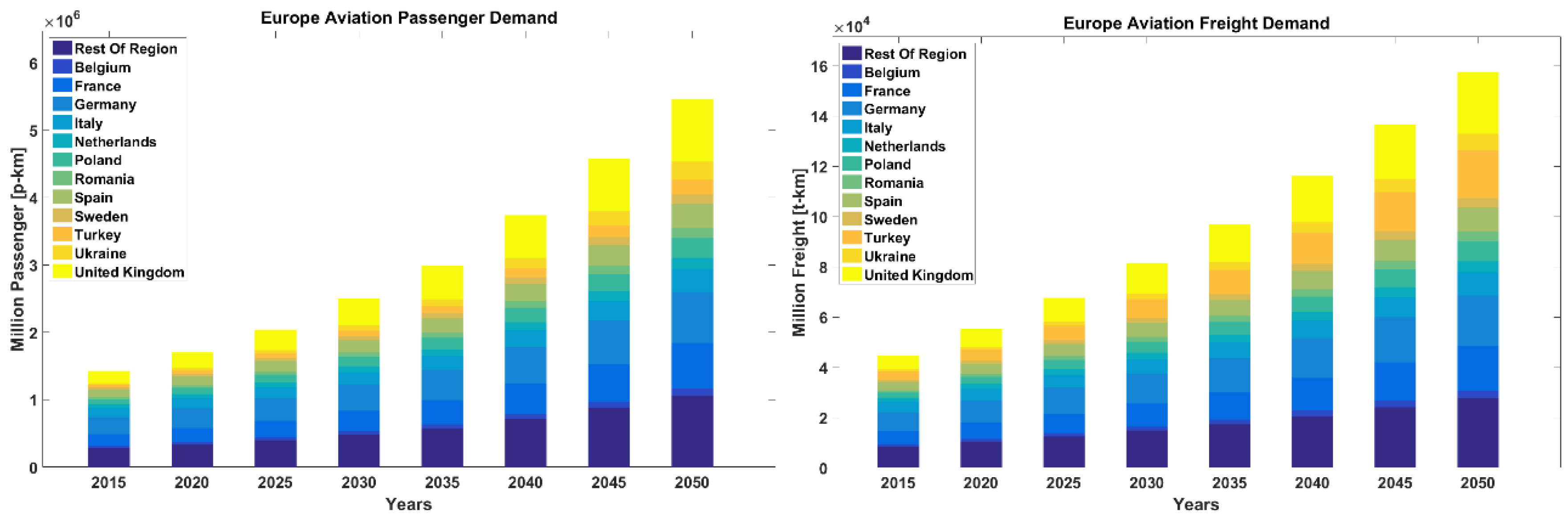
2.1.4. Aviation Transportation Activity

For the aviation passenger activity, the ICCT roadmap [64] from 2000 to 2050 is used. The metric used by ICCT is revenue passenger kilometers (rp-km), which is almost identical to the used p-km metric, not accounting for pilot and flight attendants, which seems acceptable as a first order proxy. Thus, rp-km has an identical concept as p-km from a statistical standpoint and it is used as passenger demand. The aviation t-km demand is excluded in the ICCT roadmap, but extracted from the International Civil Aviation Organization (ICAO) [71]. Based on ICAO, 197,549 million t-km transportation demand has been handled in the global aviation industry in 2015. Airfreight demand is projected to grow by 6% per year until 2035 according to ICAO [72]. From 2040 to 2050, annual growth rates of 6.4% and 6.0% and 5.5% for 2040, 2045, and 2050, respectively, are considered to be it was evaluated that the global GDP may grow approximately 4–5% per year in that period, as also adopted by Toktarova et al. [63] and airfreight demand experiences a moderately swifter growth rate than GDP.

Equation (4) indicates how aviation freight transportation demand is projected to develop in the period 2015 to 2050.

$${\left(t\text{-}km\right)}_{G_{,t+1}}={\left(t\text{-}km\right)}_{G,t}\left(1+\mathrm{GR}\right){}^{yea{r}_{t+1}-yea{r}_t}$$

(4)

wherein, ${\left(t\text{-}km\right)}_{G_{,t+1}}$ is the global aviation freight transportation demand for the following time steps, which is typically an interval of 5 years in this research, GR is the growth rate for aviation freight transportation demand, year_t+1 and year_t represent the concrete years of each step. The aviation freight transportation demand from 2015 to 2050 is distributed across countries to obtain the freight transportation demand for each country individually, as indicated in Equation (5).

$${\left(t\text{-}km\right)}_{i,t}={\left(t\text{-}km\right)}_{G,t}·\frac{\left(GD{P}_{i,t}cap·P_{i,t}\right)}{\left(GD{P}_{G,t}cap·P_{G,t}\right)}$$

(5)

wherein, ${\left(t\text{-}km\right)}_{i.t}$ is a freight demand of a country i for a point t in time, $GD{P}_{i,t} cap$ and $P_{i,t}$ is the GDP_cap and population of country i for a point t in time, the subscript $G$, represents the respective global. The regarded time period is from 2015 to 2050 and typically applied for intervals of 5 years.

Table 4. Global transportation activity for aviation passenger [64] and freight [71,72] from 2015 to 2050.

Transport Modes	Unit	2015	2020	2025	2030	2035	2040	2045	2050
Aviation Passenger	b p-km	5629	6866	8335	10,665	13,131	17,024	21,520	26,363
Aviation Freight	b t-km	198	264	354	473	634	863	1157	1514

summarizes the transportation demand values for passenger and freight in the aviation industry during the transition period until 2050, in 5-year intervals. Detailed numbers for all countries can be found in the Supplementary Material (Table S1).

The total global passenger transportation demand and freight transportation demand through the transition from 2015 to 2050, summarizing Table 2, Table 3 and Table 4 is shown in Figure 1.

2.2. Specific Energy Demand

Specific energy demand of each segment is the next step to finally derive energy demand in the transport sector. Energy demand is expressed in electrical (-_el) and thermal (-_th) units, followed by a fuel specification for thermal units, such as TWh_th,H2, TWh_th,CH4, TWh_th,liq, for hydrogen, methane, and liquid fuels, respectively. All thermal energy units are provided and used in lower heating values (LHV). Specific energy demand units can be in (MJ, kWh)/(p-km, t-km). Specific energy demand estimations are analyzed for each transport mode, segment, and power train for the transition period.

2.2.1. Road Specific Energy Demand

Heywood et al. [73] provide estimates for LDV fuel consumption in (liters/100 km) and in (kWh/100 km) for all power trains until 2050. The vehicle specific demand is linked to the number of passengers per vehicle, so that the specific energy demand in units of kWh/p-km is derived. Vehicle numbers and its occupancy known as load factor, or average people per vehicle and average freight in ton per vehicle, is extracted from Greenpeace [34] and ICCT [64], for the period until 2050. The global weighted average of load factors is calculated by the global summation of vehicle occupancy multiplied by the respective vehicle numbers of a country and then divided by the total global number of respective vehicles. The units used in this research for the specific energy demand are kWh_th/p-km, kWh_el/p-km, and kWh_H2/p-km for ICE, BEV, and FCEV, respectively. In case of PHEV, the electric driving range also influences the utility factor, also called electric driving share, as described by Plötz et al. [17,74]. The utility factor is calculated to be 0.7 for the battery-electric range of current vehicles with about 10 kWh of battery capacity [19] and is expected to grow to 0.78 by 2050. The specific energy demand for the thermal and electric parts of PHEV is based on the values for ICE and BEV. The number of passengers per vehicle is not varied for LDV of different power trains.

The energy consumption for 2W/3W BEV is estimated to be around 3–5 kWh_el/100 km for present vehicles according to [9], which is considered to be a constant value for the entire transition period. Mendes et al. [75] show that the specific energy consumption for 2W/3W ICE is 65% higher than for the BEV power train, and is also assumed constant throughout the transition period, and provided in units of kWh_th/p-km. The global weighted average of vehicle occupancy for 2W/3W is calculated in a comparable way as for LDV.

The specific energy consumption for BUS is taken from CIVITAS [76], in units of kWh/km for all power trains. The projection is available until 2030 and from then on is extrapolated based on the decrease rate from 2015 to 2030 for all power trains, excluding BUS PHEV, which is composed by BUS ICE and BUS BEV. The utility factor for BUS PHEV is taken from [77] as a constant value of 0.5 throughout the transition period. The specific energy demand for BUS PHEV is composed of the respective BEV and ICE values. Equations (6a) and (6b) show the extrapolation.

$$DR={\left(\frac{SE{D}_{t_m}}{SE{D}_{t_0}}\right)}^{\frac{1}{t_m-t_0}}-1$$

(6a)

$$SE{D}_{t_k}=SE{D}_{t_{k-1}}·{\left(1+DR\right)}^{t_k-t_{k-1}}$$

(6b)

wherein, DR is the decline rate, SED is the specific energy demand, t_m is the year with the last provided data, t₀ is the beginning of the transition period, t_k is a year within the transition period. The BUS occupancy and its projection until 2050 is done similarly to LDV.

The specific energy consumption of MDV BEV and HDV BEV is estimated to be 100 kWh/100 km and 200 kWh/100 km in 2012, according to Boer et al. [78]. The specific energy demand is projected according to Equation (6a) and (6b) using decline rates from LDV BEV. Specific energy demand for MDV ICE and HDV ICE is 4.8 and 1.6 MJ/t-km for 2015 and 2.7 and 0.8 MJ/t-km for 2050, adopted from [34]. Fulton [79] investigated that FCEV trucks have 40% lower consumption compared with ICE trucks. Load factors for MDV and HDV to translate kWh/km units to kWh/t-km units are obtained in a similar way as the passenger number per LDV, though here for ton per MDV and HDV. The utility factors for MDV PHEV and HDV PHEV are considered from [77] as a constant value of 0.4 and 0.3, respectively, throughout the transition period. The specific energy demand for MDV PHEV and HDV PHEV is composed of the respective ICE and BEV values.

Table 5. Sources for the specific energy consumption and load factors of road vehicles. Detailed numbers for all assumptions can be found in the Supplementary Material (Table S1).

Vehicle	Item	Unit	Reference
LDV	Energy consumption	kWh/100 km	[73]
	Load factor	passengers per vehicle	[34,64]
2W/3W	Energy consumption	kWh/100 km	[9,75]
	Load factor	passengers per vehicle	[64]
BUS	Energy consumption	kWh/km	[76]
	Load factor	passengers per vehicle	[1]
MDV	Energy consumption	kWh/km	[34,78,79]
	Load factor	ton per vehicle	[64]
HDV	Energy consumption	kWh/km	[34,78,79]
	Load factor	ton per vehicle	[64]

summarizes the used references for the specific energy consumption and load factors of road vehicles.

2.2.2. Rail Specific Energy Demand

Trains are divided into two power trains, electric and diesel, and this is applied for passenger and freight transport. Schäfer et al. [80] introduced a specific energy demand scenario for passenger and freight electric trains and provide specific energy demand for the years 2010 and 2050, which is considered for this research. They have also investigated that electric trains are between 45–50% more energy efficient than diesel-fueled trains, which is applied in this research. It is assumed that the specific energy demand for trains declines in a linear rate, so that all periods between 2010 and 2050 can be linearly interpolated.

2.2.3. Marine Specific Energy Demand

Marine transportation is taken into account with three power trains ICE, battery electric, and fuel-cell electric, whereas ICE can be fueled by diesel and LNG, and the fuel cells by hydrogen. For the specific energy demand for marine freight, IMO [65] introduced the absolute fuel consumption of all vessel types for 2012, which is accounted to 274,700 kt of bunker fuel, for both domestic and international shipping. Calorific values in kJ/g for heavy fuel oil, marine diesel and gas oil are provided by DNV GL [81]. Marine freight transportation demand is adopted from Section 2.1.3 and adjusted to 2012 values, so that the specific energy consumption is obtained. Horvath et al. [36] provide efficiency values for marine diesel engines for 2030 and 2040 to be 46% and 47%, respectively, and for 2050, 48% is assumed. This efficiency development is used for specific energy demand projection.

A comparison between the mechanical and electrical drives in ships is presented by Fireman and Arbor [51], introducing relative drag coefficients and propeller efficiency for both propulsion options, leading to about 65–70% efficiency. This is linked to a fuel-to-power efficiency of 40% [36] and battery full charge cycle efficiency of 92%, resulting in a total power train efficiency of about 28% and 60% for ICE and battery-electric ships, respectively for 2015. The ratio of battery electric to ICE efficiency develops from 2.16 to 1.80 from2015 to 2050. This ratio of relative efficiency can be used to obtain the specific energy consumption for freight battery-electric ships. The same procedure is adopted for hydrogen-based fuel-cell ships, though fuel-to-H₂ efficiency is assumed to increase from 53% to 65%, from 2030 to 2050, based on [36]. The respective ratio of fuel-cell to ICE efficiency for ships develops from 1.08 to 1.27, from 2030 to 2050. In terms of marine passenger specific energy demand, Becken [82] indicated that for a couple of marine passenger transport types, including ferries and cruise ships, the average value is about 2.5 MJ_th/p-km for 2010. The marine passenger specific energy demand is projected in comparable correlation as freight marine, for battery electric and fuel-cell electric ships.

2.2.4. Aviation Specific Energy Demand

The specific energy consumption of ICE, battery electric and FC planes for passenger and freight transportation is estimated. The ICCT roadmap provides aviation data in units of (revenue passenger km) rp-km/kg jet fuel consumption. As a first order approximation rp-km/kg is considered to be p-km/kg. Net calorific value is defined for jet fuels in [83], which is regarded in units of MJ/kg. ICCT [64] provides data for kg of jet fuel needed to enable respective p-km, which leads to the desired specific energy demand for ICE planes in MJ/p-km.

For electric airplanes, there is a need to use batteries for power supply, which leads to an efficiency enhancement from 30% to 80% from turboprop engine to a full battery-electric system, according to Mueller et al. [84]. They also investigate the efficiency increase of ICE to hydrogen-based FC and obtain a development from 30% to 41.7% overall efficiency. The specific energy demand for battery electric and FC planes is estimated by these efficiency ratios of battery electric and FC planes to ICE planes.

Table 6. Sources to calculate the specific energy demand for the transport modes rail, marine, and aviation. Detailed numbers for all assumptions can be found in the Supplementary Material (Table S1).

Modes	Item	Unit	Reference
Rail	Specific energy demand	MJel/p-km	[80]
	Specific energy demand	MJel/t-km	[80]
Marine	Bunker fuel consumption	kilo ton	[65]
	Calorific value	kJ/g	[81]
	Efficiency	%	[36,51]
	Specific energy demand	MJth/p-km	[82]
	Specific energy demand	MJth/t-km	[82]
Aviation	Calorific value	MJth/kg	[83]
	Efficiency	%	[84]
	Specific energy demand	MJth/p-km	[83,84]
	Specific energy demand	MJth/t-km	[83,84]

summarizes all references used to derive specific energy demand for the transport modes rail, marine, and aviation.

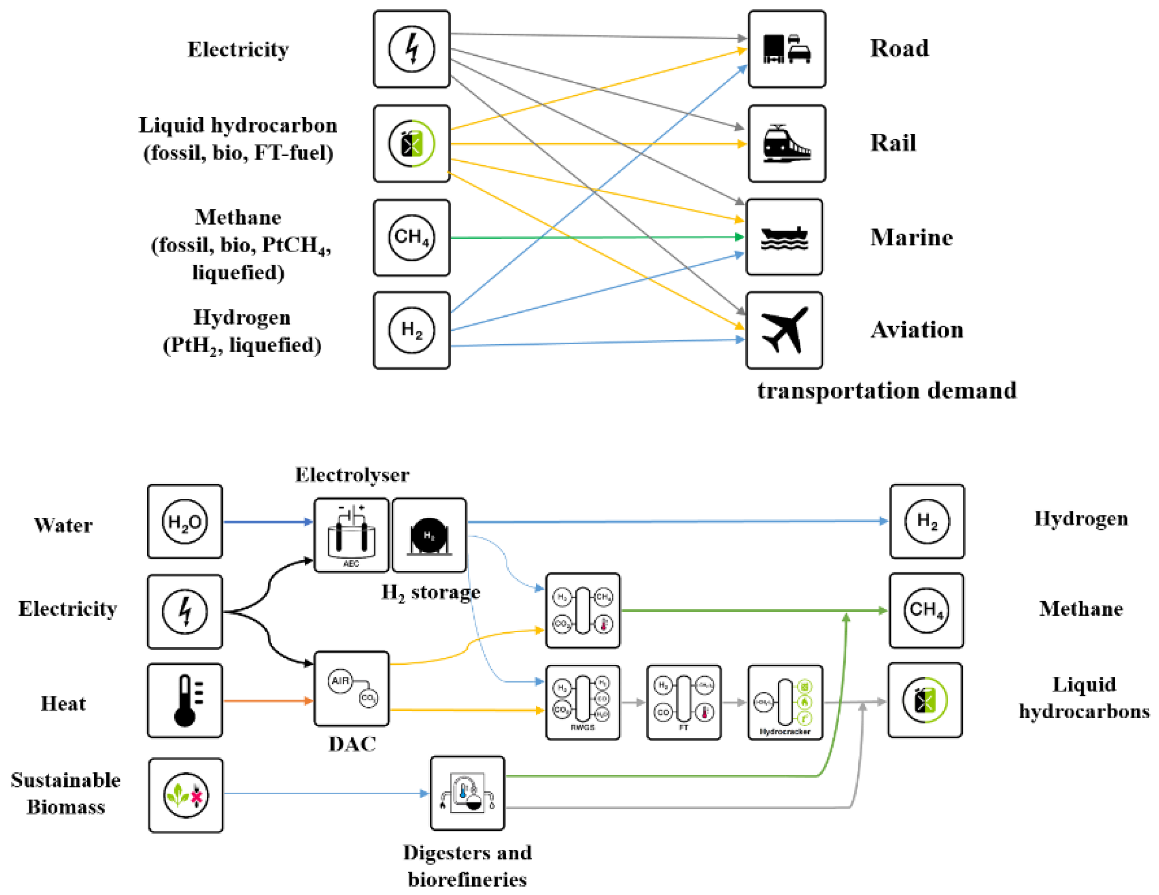
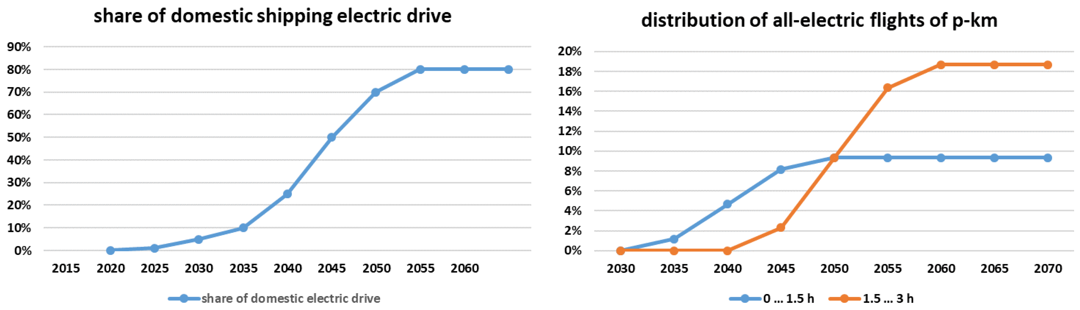
2.3. Fuel-Share Distribution of Transport Modes

The above-mentioned approaches are used to collect and calculate the transportation demand and specific energy demand for each transport mode. Thereafter, transportation demand is converted to energy demand with estimated fuel shares for the transition from the current form to sustainable and zero GHG emitting fuels throughout, until 2050. Sustainable production routes for all required fuels are established to link primary energy supply to final energy fuel demand. The following fundamental fuel types and its sustainable production routes are taken into consideration and depicted in Figure 2:

• Road: electricity, hydrogen, liquid fuels (liquid hydrocarbons)
• Rail: electricity, liquid fuels (liquid hydrocarbons)
• Marine: electricity, hydrogen, methane, liquid fuels (liquid hydrocarbons)
• Aviation: electricity, hydrogen, liquid fuels (liquid hydrocarbons)

Road transport can be powered by electricity, liquid fuels, and hydrogen. These fuels contribute with different shares through the years and complement each other. Share of each transport vehicle type within newly sold vehicles portfolio is estimated based on expected levelized cost of mobility (LCOM). The vehicles stock numbers are based on the historic structure and vehicles lifetimes, whereas newly sold vehicles substitute the existing stock at the end of their lifetimes, plus additional vehicles to satisfy a potentially growing transportation demand. Conversion to stock numbers is performed based on these newly sold vehicle shares and estimation of the total number of vehicles needed to satisfy the respective transportation demand. To calculate country wise vehicles portfolios, the respective country transportation demand is divided by respective passengers per vehicle (or freight per MDV/HDV), and average annual distance per vehicle (Equation (7a)). The number of newly sold vehicles for a respective year is comprised by the growth of the entire vehicle fleet and the reinvested vehicles (Equation (7b)). Vehicles fleet growth is calculated in comparison to the previous period (Equation (7c)). Reinvestment of vehicles is equal to vehicles expected to be decommissioned at the end of their lifetimes and respective need for substitution (Equation (7d)). The number of new vehicles of each type is the product of the share of vehicle type in newly sold vehicles and the respective number of new vehicles added in that period. Stock numbers are the sum of newly sold vehicles during the expected lifetime of vehicles. Detailed numbers for all assumptions and countries can be found in the Supplementary Material (Table S1).

$$T{F}_{i,j,t}=\frac{D_{i,j,t}}{PP{V}_{i,j,t}·DP{V}_{i,j,t}}$$

(7a)

$$N{V}_{i,j,t}=F{G}_{i,j,t}+F{R}_{i,j,t}$$

(7b)

$$F{G}_{i,j,t}=T{F}_{i,j,t}-T{F}_{i,j,t-1}$$

(7c)

$$F{R}_{i,j,t}=F{G}_{i,j,t-lifetim{e}_j}$$

(7d)

wherein, TF_i,j,t is the total fleet per road segment j and country i and year t as an integer, D_i,j,t is the transportation demand, PPV_i,j,t is passengers (or freight) per vehicle, DPV_i,j,t is average annual distance per vehicle, NV_i,j,t is the number of newly sold vehicles in the total fleet, FG_i,j,t is the number of newly sold vehicles to satisfy the growth of the vehicle fleet, FR_i,j,t is the number of newly sold vehicles to substitute decommissioning of vehicles, t is the respective year, t − 1 is the previous period, lifetime is the lifetime of vehicles. Road segments j are: LDV, 2W/3W, BUS, MDV, and HDV. The countries i are all countries in the world. The years t are from 2015 to 2050, in intervals of 5 years.

Rail transportation is based on the fuel types, electricity, and liquid fuels, applied to the shares of passenger and freight transport. The applied electricity and liquid-fuel shares for the rail mode until 2050 are taken from Greenpeace [34]. This leads to electricity and liquid fuel shares for the rail modes in 2050 of 86% and 14%, respectively.

Presently, the marine mode is practically powered solely by liquid fuels for both passenger and freight transport, neglecting small shares of methane-based LNG [85] and electric ships [86]. From 2020 onwards electricity, methane, and hydrogen will play an increasing role as alternative fuels. For electric ships, a mileage limitation to maximum of 100 km on a single charge of lithium batteries is expected [87,88]. Hydrogen and methane-based LNG are not limited in mileage. The transportation share of low range trips for ships is evaluated for deriving the electricity contribution for the marine mode. Based on GHG emissions shares of international and domestic shipping [89], it is obtained that 11% of the total shipping is domestic and it is assumed that 80% of all domestic shipping is within a range for electrification. The assumed phase-in of electric domestic ships is visualized in Figure 3. In accordance with this assumption and marine transportation demand, the share of electric shipping is calculated.

Currently, aviation transportation is entirely based on liquid fuels. This will have to change in the upcoming decades for responding to the climate emergency but also due to economic reasons. From around 2035 onwards, it is assumed that hydrogen and electricity start to gain market shares for powering airplanes, as documented by first policies for all-electric flights in Norway with up to 1.5 h range [52] and expectations in technology enhancement for flights up to 3 h [90]. Electric airplanes are limited in range due to the limited energy density of lithium batteries. Short haul flights up to 1.5 to 3 h with utmost 100 passengers have the potential to be electrified according to Wilkerson et al. [91] and Mueller et al. [80]. Consequently, this research assumes for 2050 that 18.7% of the flights measured in passenger kilometers representing short haul flights of less than 1.5 h and half of the flights between 1.5 and 3 h will be electric and twice that is assumed to be contributed by fuel-cell-based flights fueled by hydrogen (37.4%), while the rest representing the majority of all p-km for flights is projected to remain powered with jet fuel. The phase-in of all-electric flights is visualized in Figure 3, and based on the estimate of 11.7% of all p-km for flights up to 1.5 h and 23.4% of all p-km for flights within 1.5 and 3 h, whereas 80% of these flights should be served by all-electric flights in the longer term, which is projected to be achieved between 2050 and 2060. The assumed progress in aviation technology and respective implementation is based on today’s understanding of technological options [84,90,91], first respective policies [52] and the enormous pressure to react on climate emergency [2,69,92,93], while economics may be attractive and first leading technology providers and airlines push the development to introduce all-electric flights by 2030 [94].

2.4. Capital Expenditures, Operational Expenditures, and Lifetimes for Road Vehicles

In this paper, the LCOM for road vehicles is used to obtain the evolution of the vehicle types. Capital expenditures (capex) for the vehicle types of LDV, BUS, MDV, and HDV and their respective projections from 2015 to 2050 are considered. This evaluation is done for four mentioned segments and the following power trains: ICE, BEV, PHEV, and FCEV. In addition, operational expenditures (opex) for all vehicle types and lifetimes are considered.

Capex, opex, lifetime and weighted average cost of capital (WACC) form the key performance unit LCOM, so that all vehicle types within a vehicle class can be compared. LCOM is defined in Equation (8). Opex variable is defined in Equation (9). The capital recovery factor (crf) used for LCOM is defined in Equation (10). WACC is set at 7% in this study. GHG emissions cost (GHG_cost) are adopted from Bogdanov et al. [95].

$$LCOM=\frac{\left[\left(cape{x}_{tot}-cape{x}_{bat}\right)·cr{f}_{tot}+cape{x}_{bat}·cr{f}_{bat}+ope{x}_{fix}\right]}{\mathrm{mileage}}+ope{x}_{var}$$

(8)

$$ope{x}_{var}=E_{cons}·E_{cost}+GH{G}_{emit}·GH{G}_{cost}$$

(9)

$$crf= \frac{\mathrm{WACC}·{(1+\mathrm{WAC}C)}^N}{{(1+\mathrm{WAC}C)}^N-1}$$

(10)

wherein, capex_tot is total capital expenditure of vehicle, capex_bat is battery capex of vehicle, opex_fix is the fixed operational expenditure of vehicle, mileage is the annual mileage of vehicle, opex_var is the variable operational expenditure of vehicle, E_cons is the specific energy demand per km of vehicle, E_cost is the specific cost of fuels used by vehicle, GHG_emit is the specific emitted GHG emissions per km, GHG_cost is the applied CO_2eq price, and mileage is the annual mileage of vehicle.

2.4.1. Capital Expenditures

Vliet et al. [96] investigated the regular diesel and gasoline prices in euros for LDV ICE vehicles. Vehicles consist of two major parts: platform and power train. The two liquid-fuel LDV types are averaged in the following, and constant cost for LDV ICE platform and power train are assumed over the entire transition period. The capex of LDV BEV are split into three main components: platform, electrical drive, and battery. The specific cost of the battery is high in the beginning, but a continued and drastic cost reduction is factored in, based on Bloomberg New Energy Finance (BNEF) [97] and UBS [19]. The starting specific cost of the battery is 198 €/kWh_cap in 2017 [19,97]. A cost reduction of 7.9% per year is assumed until 2030, based on BNEF and UBS assumptions, and 2% per year until 2050. The obtained specific battery cost for 2030 is confirmed by Nguyen and Ward [98]. The power train cost reduction is assumed at 7.9% per year until 2030 and 2% per year then onwards [19,97]. LDV PHEV is composed by ICE and BEV components, but with lower battery capacity. The cost reduction of the power train and battery is assumed to follow the same percentage as for LDV BEV. The battery capacity for BEV and PHEV is calculated to be 70 and 10 kWh, respectively by multiplying all-electric range km of the vehicle to its specific efficiency in kWh/km [19]. LDV FCEV vehicles consist of the major components: platform, power train (fuel cell and electric motor) and hydrogen energy storage. The platform cost is adopted from Vliet et al. [96], with a fuel-cell power of 100 kW and a range of about 500 km, leading to a hydrogen storage capacity of 140 kWh_H2. Assumptions for the power train and hydrogen storage are considered from Bubeck et al. [99]. The fuel tank capex is considered to be fixed at 1.9 €/kWh_H2, whereas the power train capex declines from 284 €/kW in 2015 to 48 €/kW in 2050, according to estimates of UBS [19].

BUS ICE capex is adopted from Lajunen and Lipman [100] and constant capex for the entire transition period is assumed. The platform cost share of BUS ICE is extracted from LDV platform cost share, according to Vliet et al. [96] and found to be 74% of the total capex, so that the other BUS power train types can be investigated. BUS BEV is composed of the platform capex plus the power train and battery. The platform cost of BUS BEV is identical to BUS ICE, and the BUS BEV battery cost is calculated by multiplying the battery capacity in kWh [100] with the specific battery cost. The reduction of battery cost for the BUS BEV by 2050 is according to the LDV method. BUS BEV power train capex is the same value as for BUS PHEV, which is described in Equation (11). BUS BEV battery capacity is set to 333 kWh, according to Lajunen and Lipman [100], assuming the identical specific battery capex cost reduction as in LDV BEV. BUS PHEV capex components are split to the components: platform, battery, and power train (ICE and BEV). The platform cost is identical for all BUS vehicle types. Battery capacity is set to 49.7 kWh, according to Lajunen et al. [101] and the specific battery capex cost decline is assumed to be identical to LDV BEV. The BUS PHEV power train is calculated according to the respective development of LDV, but based on BUS assumptions, as detailed in Equation (11), which can be applied for all years of the transition period.

$$\begin{array}{c}cape{x}_{powertrain,BUSPHEV,year}\hfill \\ =\left(cape{x}_{total,BUSICE}-cape{x}_{platform,BUSICE}\right)·\frac{cape{x}_{powertrain,LDVPHEV,year}}{cape{x}_{powertrain,LDVICE,year}}\hfill \end{array}$$

(11)

wherein, capex is capital expenditures for the power train, the entire bus, total, and the platform., and year indicates the considered year in the transition period.

Current BUS FCEV capex are adopted from Lajunen [101], leading to a cost decline of the vehicle, excluding the platform, of 5% per year up to 2030, based on Vliet et al. [96]. As technological similarities exist, a further cost decline of 2% from 2030 to 2050 is presumed. Finally, the aggregation of all components per BUS type leads to the total capex for each year within the transition period.

MDV ICE capex is assumed to stay stable, according to Yeon and Thomas [102], from which the class 6 vehicle is regarded. In analogy to BUS, the LDV platform share of 74% is also applied for MDV vehicles. MDV BEV capex is composed of three capex contributions from the platform, power train, and battery. The platform capex is identical to MDV FCEV. MDV BEV power train is estimated as the ratio of LDV BEV power train capex to LDV BEV platform capex, applied to the MDV BEV platform capex. The specific battery capex is assumed identical to LDV BEV, but for a battery capacity of 120 kWh [103]. The MDV PHEV capex is composed with the same logic as in LDV PHEV and MDV in general. The MDV PHEV platform capex is identical to MDV BEV, i.e., 74% of the total capex of MDV ICE. MDV PHEV power train capex is calculated similarly to Equation (11). The MDV PHEV battery capacity is taken as the MDV BEV battery capacity multiplied by the ratio of the battery capacities of LDV PHEV to LDV BEV, while the identical specific battery capex is assumed. MDV FCEV electric motor is set to 170 kW for the class 6 vehicle, according to Kast et al. [104], and the respective capex decline follows the percentage of LDV FCEV. The MDV FCEV hydrogen storage capacity is scaled according to the specific energy demand of MDV FCEV versus LDV FCEV and the identical specific hydrogen storage capex is assumed. The sum of the three capex components yields the total capex of MDV FCEV, which is then applied for all years within the transition period.

Capex for HDV ICE is regarded as the average capex of several heavy-duty trucks, according to Laitila et al. [105]. The method is identical to MDV. Specific values are HDV FCEV electric motor of 250 kW [104] with a capex decline according to MDV FCEV. Tesla [106] claims that by 2020 there will be 900 kWh battery capacity for their HDV BEV for 143 €/kWh_cap, which is set as a reference, while the relative battery capex decline is assumed to be according to LDV BEV. The battery capacity for HDV PHEV is estimated according to the same method as in MDV PHEV, as also for the other components.

2.4.2. Operational Expenditures

Opex fixed comprises of insurance and maintenance cost for the vehicles, and no change in the insurance cost is assumed throughout the transition period. The annual insurance cost for LDV ICE [107] is assumed to be the same for all LDV types. LDV BEV maintenance cost is lower than for LDV ICE due to reduced complexity [108]. LDV ICE and LDV BEV maintenance costs are assessed in [53] and used in this study. LDV PHEV maintenance cost is comprised of the full LDV ICE maintenance cost plus half the maintenance cost of LDV BEV. LDV FCEV maintenance cost is assumed to be comparable to ICE and BEV, thus comprising half of each.

Insurance cost for BUS is taken from [109] and assumed to be identical for all BUS types. BUS ICE maintenance cost is taken from [100], as 0.16 €/km for an annual distance of 66,667 km. Maintenance costs for BUS BEV, PHEV, and FCEV are based on BUS ICE and scaled according to the LDV types. Insurance costs for MDV ICE and HDV ICE are taken from [110], whereas the respective classifications for MDV and HDV are taken from [104]. MDV ICE maintenance costs for diesel MDV is estimated to be between 300 to 600 USD/month, therefore 450 USD/month are applied and converted by long-term average currency exchange rate of 1.3 USD/€. Other MDV type maintenance cost is scaled in accordance to LDV. HDV ICE insurance cost is set identical to all HDV types and taken from Bento et al. [111]. HDV maintenance cost is set to be identical to BUS for all HDV types.

Table 7. Sources used for vehicle, battery, and hydrogen storage prices as well as maintenance and insurance costs.

Vehicle	Item	Unit	Reference
LDV	Vehicle price	€	[96]
	Battery/hydrogen price	€/kWh	[19,97,98,99]
BUS	Vehicle price	€	[100]
	Battery/hydrogen price	€/kWh	[100,101]
MDV	Vehicle price	€	[102]
	Battery/hydrogen price	€/kWh	[104]
HDV	Vehicle price	€	[105]
	Battery/hydrogen price	€/kWh	[104,106]
All types	Insurance	€/vehicle	[107,109,110]
	Maintenance	€/vehicle	[19,100,108]

provides all sources used for capex and opex for all road vehicle types. The calculations of vehicle, battery and hydrogen storage capex as well as maintenance and insurance costs are presented in the Supplementary Material (Table S1).

2.4.3. Lifetime

Vehicle lifetime is determined as an average vehicle age from starting operation to scrappage stage. Vehicle lifetimes for all vehicle types are assumed to stay constant until 2050. Battery lifetime must be considered for all BEV and PHEV road segments. Changes in scrappage patterns for LDV and the consequence of a higher average lifetime is discussed by Bento et al. [105]. However, Dun et al. [112] point out that vehicle lifetime heavily depends on annual mileage, which is assumed to be roughly 10,000 km for LDV. Battery lifetime is assumed to be identical for BEV and PHEV, as discussed by Guenther et al. [113]. Laver et al. [114] discuss the concept of useful lifetime for BUS, which is concluded to be between 12 and 14 years. In this study, the planned useful lifetime chosen is a bit longer to also cover the period until decommissioning. Lajunen [101] describes 80,000 km for the BUS battery lifetime in case of city operation, which can be translated to 3000–12,000 full charge cycles or 5–10 years [115,116,117]. 2W/3W vehicles lifetimes are taken from [9]. Battery installed in 2W/3W vehicles can be valve-regulated lead-acid (VRLA) or lithium-ion battery with different lifetimes, whereas lithium-ion technology is assumed as the standard, also due to more promising future and longer lifetime in mobile applications, according to Weinert et al. [118]. MDV lifetime is similar to LDV decommissioning age, and average age of MDV is taken from [119]. HDV lifetime is slightly longer than that of MDV or LDV [114,119].

Table 8. Vehicle lifetime for all road segments.

Vehicle	Unit	2015–2050	Reference
LDV	years	15	[111,112]
2W/3W	years	10	[9]
BUS	years	15	[114]
MDV	years	15	[119]
HDV	years	16	[114,119]

and

Table 9. Battery lifetime for all technologies on the road.

Vehicle Type	Unit	2015–2050	Reference
LDV BEV	years	10	[113]
LDV PHEV	years	10	[113]
2W/3W BEV	years	9	[9]
BUS BEV	years	9	[101]
BUS PHEV	years	6	[101]
MDV BEV	years	10	[113]
MDV PHEV	years	5	[113]
HDV BEV	years	10	[113]
HDV PHEV	years	5	[113]

summarize the vehicle and battery lifetimes for all road segments and vehicle types.

2.4.4. Annual Kilometers for the Road Segment

The annual kilometers driven per vehicle type is the weighted average kilometers of vehicle types with their occupancy and number of vehicles for all countries globally.

Table 10. Annual kilometers per vehicle.

Vehicle Type	Unit	2015	2020	2025	2030	2035	2040	2045	2050
LDV	km/a	14,603	14,004	13,357	12,993	12,728	12,468	12,217	11,971
2W/3W	km/a	7224	7380	7453	7494	7435	7427	7480	7702
BUS	km/a	64,744	67,178	68,854	70,810	72,610	74,503	76,293	77,465
MDV	km/a	25,389	26,154	26,631	27,140	27,601	28,058	28,416	28,655
HDV	km/a	54,541	53,521	52,941	52,582	52,188	51,747	51,312	50,866

summarizes the annual kilometers for all road vehicles. Detailed numbers for all countries can be found in the Supplementary Material (Table S1).

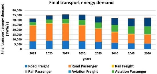
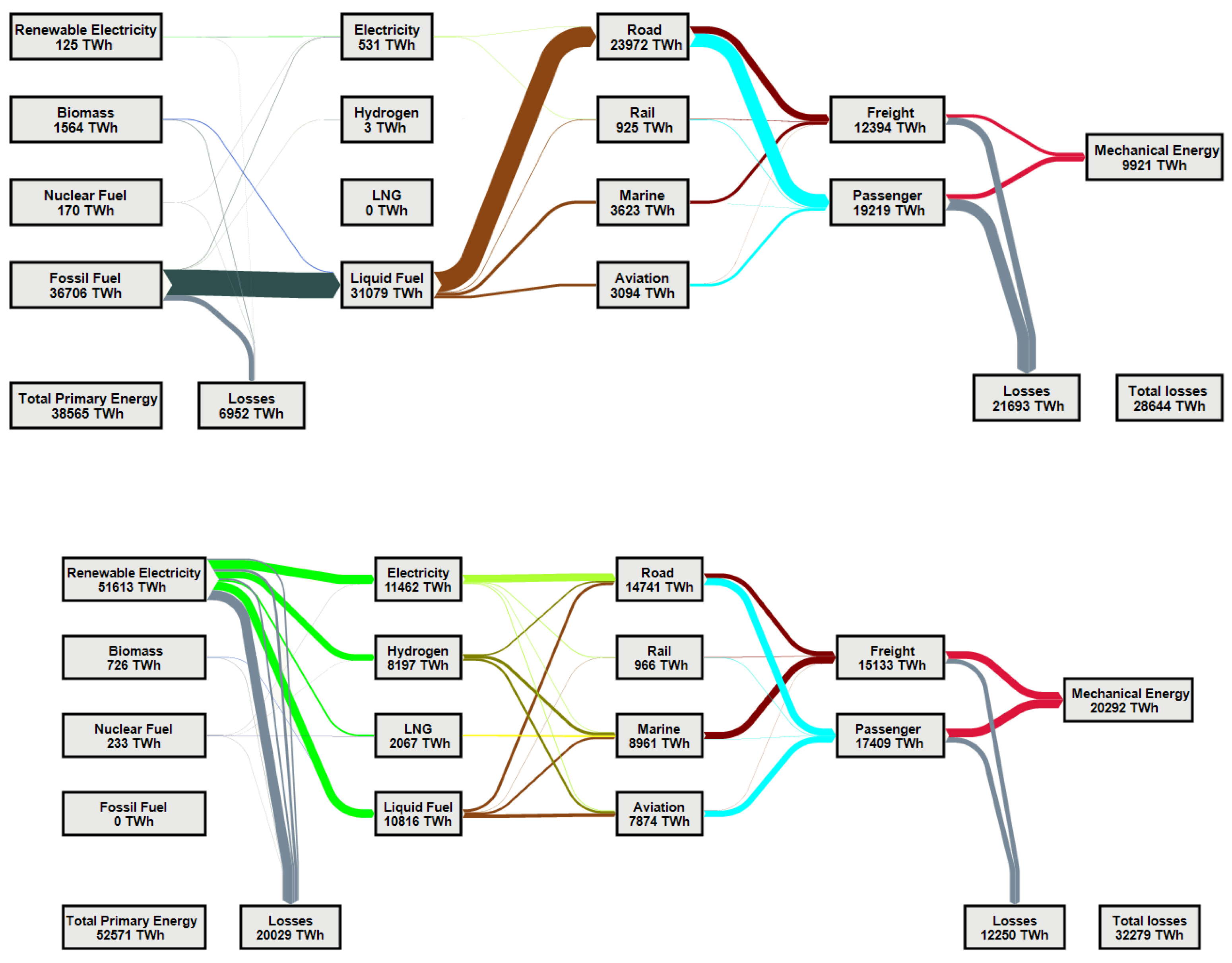
2.5. Global Final Energy Demand in the Transport Sector

The final energy demand for the transport sector can be derived on basis of transportation activities, specific energy demand for each transport mode with all transport segments and vehicle types, and the respective fuel-share distribution. The GHG emission intensity of the used fuels further determine the GHG emissions of the transport sector. An overview diagram of the key factors, from transportation activity to total final energy demand and GHG emissions via specific energy demand and fuel-share distribution is visualized in Figure 4.

The final energy demand is calculated according to Equation (12), which allows a detailed consideration of all transport activities of the different transport modes and segments, the differentiation of vehicle types, the evolution of fuel shares and the development of the specific energy demand per vehicle type, fuel, and segment. The structure of Equation (12) is also visualized in Figure 4. This calculation can be carried out per geographic entity, for instance a country, and then aggregated to larger regions, continents, and the world. Detailed numbers for all input data can be found in the Supplementary Material (Table S1).

$$E_{FD,year}={\displaystyle \sum }_{i,s,v,f}^{}T{A}_{i,s}·V{T}_v·F_{i,s,v,f}·E{D}_{i,s,v,f}$$

(12)

wherein, E_FD is the final energy demand, year is the considered year within the transition period, TA is the transport activity, VT is the vehicle type, F is the fuel-share distribution, ED is the specific energy demand and the indices are i for the transport mode (road, rail, marine, aviation), s for the transport segment (passenger, freight; for road: LDV, 2W/3W, BUS, MDV, HDV), v for the vehicle type (road: ICE, BEV, PHEV, FCEV) and f for the fuel type (electricity, hydrogen [electricity, fossil], methane [electricity, fossil], liquid fuels [electricity, biofuel, fossil]).

The final energy demand according to Equation (12) can be categorized in different ways, e.g., as the global total for all countries and all transport activities, or per country for a transport mode or transport segment, or for a specific fuel type.

The analysis can be further differentiated for the total primary energy demand of the transport sector. This requires the consideration of the conversion of primary energy sources to the final energy forms of required fuels. Figure 2 indicates this for modern synthetic fuels. For deriving the full primary energy demand, an energy supply scenario is required reflecting the development of the electricity mix, the applied hydrogen production technology, in particular electricity-based electrolysis and steam methane reforming based on fossil natural gas, the methane supply mix, in particular fossil natural gas and power-to-gas, liquid-fuel mix based on fossil fuels, biofuels, and electricity-based Fischer-Tropsch fuels. This is detailed in Section 2.7.

2.6. GHG Emissions from the Transport Sector

Well-to-wheel (WTW) GHG emissions analysis for the various fuels used is the decisive metric, since it considers the fuel value chain from primary energy to final use. WTW consists of well-to-tank (WTT) comprising fuel refining and logistic requirements from primary energy to final energy and tank-to-wheel (TTW), which comprises the GHG emissions of the final energy fuels used. GHG emission factors for fuels are taken from IPCC [120], using average values for liquid fuels comprised of diesel, gasoline, jet fuel, residual fuel oil and biofuel for the TTW balance, and fossil natural gas for LNG TTW emissions. The TTW values for hydrogen and electricity as a final energy fuel are zero. The TTW GHG emission values for LNG and liquid fuels will decline until 2050 based on the applied energy transition scenario, which can imply an electricity share for methane via power-to-gas and a renewable electricity (RE) share for liquid fuels, comprised of biofuels and electricity-based FT fuels. The shares of the various sustainable fuels are according to Section 2.3 and Section 3.2.3. WTW GHG emission intensity for liquid fossil fuels are taken from Rahman et al. [121], who averaged five North American conventional crudes, and derived values for gasoline, diesel, and jet fuel, which have been averaged for liquid fossil fuels, as used in this analysis. WTW GHG emissions from sugarcane and corn as bioethanol feedstock are taken from Wang et al. [122]. GHG emissions from palm oil as biodiesel feedstock are taken from Nylund and Koponen [123]. The finally used emission value for biofuel is the weighted average of bioethanol and biodiesel with their available market shares and represented by the main producers the USA and Brazil, as taken from [124]. WTW GHG emissions for fossil LNG is 300 gCO_2eq/kWh_th in the 100-year GWP consideration of methane emissions, as suggested by IPCC in its 5th Assessment Report and discussed here [125]. The WTW emission intensity of liquid fuels and LNG declines because of the applied energy transition scenario through an expected increase of RE shares used for these final energy fuels. Presently, hydrogen production is dominated by fossil natural gas-based SMR, leading to a WTW GHG emission of 380 gCO_2eq/kWh_H2. Similar to liquid fuels and LNG, these emissions decline as the share of used RE increases, because of the energy transition. Hydrogen from SMR is expected to be substituted by hydrogen from renewable electricity-based electrolysis, as discussed in Fasihi et al. [126] and Elgowainy et al. [127]. Electricity WTT GHG emissions, better called well-to-grid (WTG) GHG emissions, depend on the used electricity supply mix and its composition with primary fuels such as coal, fossil natural gas, fuel oil, nuclear, and the various forms of renewables. The GHG emission values of fossil oil and fossil natural gas used for the final energy fuels are also used for the electricity supply. GHG emission values for lignite coal (400 gCO_2eq/kWh_th) and hard coal (390 gCO_2eq/kWh_th) are taken from Schuller [128]. The two coal emission factors are weighted into a unified GHG emission value, based on their total global production, according to Skone [129]. The specific GHG emission values in thermal energy units are converted to the average efficiency of thermal power plants used for electricity generation. The considered thermal power plants are oil-based ICE generators, coal power plants, and open cycle and combined cycle gas turbines. All efficiency values and the assumed energy transition scenario is taken from Bogdanov et al. [95]. The energy transition scenario for the final energy fuels is according to Section 2.7 and Section 3.5. GHG emission intensities of the considered final energy fuels during the energy transition period, as obtained by applying the energy transition scenario is summarized in

Table 11. GHG emission intensity for all applied final energy fuels for TTW and WTW consideration. The remaining GHG emissions in 2050 are from biofuels and mainly due to indirect GHG emissions.

Fuel	Method	Unit	2015	2020	2025	2030	2035	2040	2045	2050
Electricity	TTW	gCO2eq/kWhel	0	0	0	0	0	0	0	0
Hydrogen	TTW	gCO2eq/kWhH2	0	0	0	0	0	0	0	0
LNG	TTW	gCO2eq/kWhCH4	237	237	237	230	194	135	54	0
Liquid fuel	TTW	gCO2eq/kWhth	266	266	266	258	218	151	71	10
Electricity	WTW	gCO2eq/kWhel	513	373	140	47	15	6	2	0
Hydrogen	WTW	gCO2eq/kWhH2	389	395	334	223	148	65	21	0
LNG	WTW	gCO2eq/kWhCH4	300	300	300	294	251	176	71	0
Liquid fuel	WTW	gCO2eq/kWhth	368	366	366	358	305	211	96	8

for TTW and WTW considerations, which also allows a WTT analysis, if required.

The total GHG emissions of the transport sector on different levels of aggregation and for different years can be calculated according to Equation (13), which is closely linked to Equation (12). The structure of Equation (13) is also visualized in Figure 4. This calculation can be carried out per geographic entity, for instance a country, and then aggregated to larger regions, continents, and the world, in the same way as for the final energy demand. The TTW, WTW, or WTT GHG emissions can be analyzed separately, by applied respective values according to Table 11. Detailed numbers for all input data can be found in the Supplementary Material (Table S1).

$$GH{G}_{total,b,year}={\displaystyle \sum }_{i,s,v,f}^{}T{A}_{i,s}·V{T}_v·F_{i,s,v,f}·E{D}_{i,s,v}·GH{G}_{f,b}$$

(13)

wherein, GHG_total is the total GHG emissions, b is the balancing of WTT, TTW, or WTW, year is the considered year within the transition period, TA is the transportation activity, VT is the vehicle type, F is the fuel-share distribution, ED is the specific energy demand, GHG_f is the specific GHG emission per final fuel, and the indices are i for the transport mode (road, rail, marine, aviation), s for the transport segment (passenger, freight; for road: LDV, 2W/3W, BUS, MDV, HDV), v for the vehicle type (road: ICE, BEV, PHEV, FCEV), and f for the fuel type (electricity, hydrogen, LNG, liquid fuels).

The total GHG emissions according to Equation (13) can be categorized in different ways, e.g., as total global for all countries and all transport activities, or per country for a transport mode or transport segment, or for a specific fuel type.

2.7. Primary Energy Demand and Well-to-Wheel Efficiency

WTW efficiency analysis for various fuels and vehicle types used is a key metric for the transport sector, since it considers the entire energetic value chain from primary energy to final mechanical use. The WTW concept consists of WTT, comprising the fuel production chain from primary energy to final energy fuels, and TTW, which comprises the final energy fuels used in vehicles. For WTT, the full life cycle chain of the fuels is evaluated for analyzing the fuel efficiency. The conversion steps comprise the principle routes from primary input to final energy fuels, as characterized in

Table 12. Overview of conversion processes from primary input to final energy fuels for the WTT perspective.

Primary Input	Conversion	Final Energy Fuel
Fossil fuels	Refinery	liquid hydrocarbons, diesel, gasoline
Fossil fuels	Power plants (coal, gas, oil)	electricity
Fossil fuels	Steam methane reforming	hydrogen
Nuclear fuels	Nuclear power plant	electricity
Electricity	Fischer-Tropsch	liquid hydrocarbons
Electricity	Electrolysis	hydrogen
Hydrogen	Methanation	methane
Methane	Liquefaction	LNG
Biomass	Biorefinery	biofuels, liquid hydrocarbons, biodiesel, bioethanol

. Primary energy is defined as the first form of energy provided by an extraction technology from nature. This applies to fossil fuels (coal, natural gas and crude oil), nuclear fuels (uranium), biofuels (biomass) and renewable electricity (solar PV, wind electricity, hydropower). Losses of power transmission and distribution are considered for all electricity generation. For renewable electricity, there are two further loss types, which are considered for the WTT value chain: curtailment and storage. Curtailment and storage losses related to renewable electricity are taken from Bogdanov et al. [95] and overall power transmission losses are taken from Sadovskaia et al. [130].

For example, if the final energy fuel is LNG, the efficiency chain from raw material extraction to the vehicle tank has to be taken into account, and in the case of renewable electricity, the electricity generation, the conversion steps, electrolyzer, methanation, and liquefaction are required and the losses due to power transmission, curtailment, and storage have to be considered.

Table 13. WTT efficiency values for all final energy fuels. Renewable electricity (RE) is mainly composed of solar PV, wind electricity, and hydropower. Conversion of fossil fuels to electricity is volume averaged for the power plant types of coal, combined cycle gas turbines, open cycle gas turbines, and internal combustion engines.

Primary Origination	Fuel Type	WTT Efficiency	2015	2020	2025	2030	2035	2040	2045	2050
Fossil	Diesel [131,132]	%	83	84	85	85	86	87	87	88
Fossil	Gasoline [131,132]	%	85	86	86	87	88	88	89	90
Fossil	Liquid Hydrocarbons	%	84	85	85	86	87	87	88	89
RE	Liquid Hydrocarbons [133]	%	n/a	n/a	n/a	53	53	53	53	53
Fossil	Electricity [95]	%	44	46	47	48	47	46	46	0
Nuclear	Electricity [95]	%	33	33	33	33	37	37	37	38
RE	Electricity [95]	%	100	100	100	100	100	100	100	100
Fossil	Hydrogen [134]	%	85	85	85	85	85	85	85	85
RE	Hydrogen [95]	%	84	84	84	84	84	84	84	84
Fossil	LNG [135]	%	85	85	85	85	85	85	85	85
RE	LNG [135]	%	57	57	57	57	57	57	57	57
Corn	Bioethanol [131]	%	61	61	61	61	61	61	61	61
Sugarcane	Bioethanol [131]	%	48	48	48	48	48	48	48	48
Palm	Biodiesel [131]	%	80	80	80	80	80	80	80	80
Biomass	Liquid Hydrocarbons	%	60	60	60	60	60	60	60	60

details the WTT efficiencies taken into account for all final energy fuels. The references indicated are used for the respective efficiencies.

Fossil liquid hydrocarbons is an average of diesel and gasoline in the ratio 1:1. Similarly, biomass-based liquid hydrocarbons is the weighted average of the two main biofuels, composed by 79% of bioethanol and 21% of biodiesel [136]. Hydrogen and LNG are considered from fossil fuels and renewable electricity with changing shares during the transition period. Electricity is supplied from renewable sources, nuclear, and fossil fuels with changing shares during the transition period from 2015 to 2050. Production route shares for the final energy fuels are indicated in

Table 14. Shares of final energy production routes.

Final Energy Fuel	Input	Contribution Share	2015	2020	2025	2030	2035	2040	2045	2050
Electricity	Fossil	%	68	50	19	7	2	1	0	0
	Nuclear	%	10	10	7	4	2	1	1	0
	Renewable	%	22	40	74	89	96	98	99	100
Hydrogen	Fossil	%	100	90	75	50	35	15	5	0
	Electricity	%	0	10	25	50	65	85	95	100
LNG	Fossil	%	100	100	100	97	82	57	23	0
	Electricity	%	0	0	0	3	18	43	77	100
Liquid hydrocarbons	Biofuel	%	3	4	4	4	4	4	4	4
	FT fuels	%	0	0	0	3	18	43	73	96
	Fossil	%	97	96	96	93	78	53	23	0

, in case more than only one route exists. Electricity is factored in according to the generation mix of the respective period.

TTW efficiency for the four transport modes is calculated to represent how much final energy can be converted by the power trains to mechanical energy and the rest is allocated as loss.

Table 15. TTW efficiencies of all vehicle types for road transport.

Vehicle	Type	TTW Efficiency	2015	2020	2025	2030	2035	2040	2045	2050
LDV	ICE [137]	%	20	22	24	26	26	27	27	28
	BEV [138]	%	74	77	81	84	86	87	89	91
	PHEV—ICE	%	20	22	24	26	26	27	27	28
	PHEV—EV	%	74	77	81	84	86	87	89	91
	FCEV [131]	%	30	34	39	43	45	47	48	50
2W/3W [139]	ICE	%	12	13	14	16	16	16	16	17
	BEV	%	44	46	48	50	51	52	53	54
BUS [140]	ICE	%	33	33	34	35	35	36	36	37
	BEV	%	73	76	79	83	85	86	88	90
	PHEV—ICE	%	33	33	34	35	35	36	36	37
	PHEV—EV	%	73	76	79	83	85	86	88	90
	FCEV	%	44	46	48	50	52	54	56	58
MDV	ICE [141]	%	32	32	33	33	34	34	35	35
	BEV [142]	%	73	76	79	83	85	86	88	90
	PHEV—ICE	%	32	32	33	33	34	34	35	35
	PHEV—EV	%	73	76	79	83	85	86	88	90
	FCEV [142]	%	45	47	49	51	53	55	57	59
HDV	ICE [141]	%	41	42	43	43	44	45	45	46
	BEV [142]	%	73	76	79	83	85	86	88	90
	PHEV—ICE	%	41	42	43	43	44	45	45	46
	PHEV—EV	%	73	76	79	83	85	86	88	90
	FCEV [142]	%	45	47	49	51	53	55	57	59

shows the TTW efficiencies for the road transport segments, while

Table 16. TTW efficiencies for the transport modes rail, marine, and aviation.

Modes	Type	TTW Efficiency	2015	2020	2025	2030	2035	2040	2045	2050
Rail, trains [143]	Electric	%	76	77	78	79	80	81	82	83
	Diesel	%	31	33	34	35	36	36	37	37
Marine, ships [36,144]	Electric	%	62	63	64	64	65	66	67	68
	Hydrogen	%	45	48	51	54	56	57	59	60
	LNG	%	45	46	48	49	50	50	51	51
	Diesel	%	42	43	45	46	47	47	48	48
Aviation, airplanes [54]	Electric	%	73	74	75	76	77	78	79	81
	Hydrogen	%	44	46	47	49	50	52	54	55
	Jet fuel	%	39	40	41	42	43	44	44	45

shows the TTW efficiencies for the transport modes rail, marine, and aviation.

3. Results

3.1. Global, Regional, and Country Level Transportation Demand

The transportation demand is structured into the four transport modes, road, rail, marine, and aviation, each for passenger and freight transportation, as detailed in Section 2.2. The geographic structuring of the global results are in accordance to Bogdanov et al. [95], for the nine major regions: Europe, Eurasia, Middle East Northern Africa (MENA), Sub-Saharan Africa, South Asian Association for Regional Cooperation (SAARC), Northeast Asia, Southeast Asia, North America, and South America. The scaling of the geographic results and aggregation is visualized in Figure 5 for the global road passenger and freight transportation demand during the entire energy transition period. The European aviation transportation demand for passenger and freight is shown in Figure 6. The marine transportation demand in France for passengers and freight is depicted in Figure 7. The disaggregated values for all countries, transport modes, and transport segments can be found in the Supplementary Material (Table S1). The global transportation demand for the transport modes rail, marine, and aviation across the nine major regions during the transition period is presented in Figure 8, Figure 9 and Figure 10. All transport modes are faced with strong global transportation demand growth, as also mentioned in Section 2.1. More detailed diagrams for the four transport modes across the nine major regions and on the country level is presented in the Supplementary Material (Figures S1–S5). All numeric details are part of the comprehensive tables in the Supplementary Material (Table S1), which allow further analyses.

3.2. Specific Energy Demand, Road LCOM, and Shares of Vehicle and Fuel Types

3.2.1. Specific Energy Demand

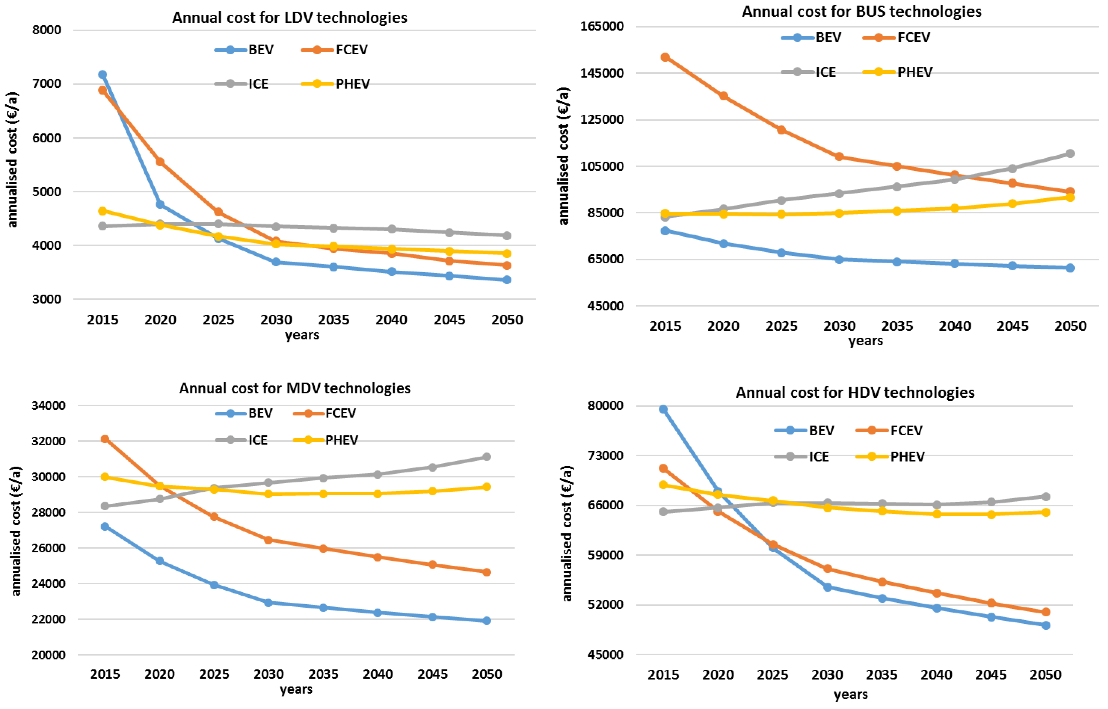
The specific energy demand and energy intensity values for all transport modes are calculated according to the methods introduced and are presented in detail in this section. Values for specific energy demand for the road transport mode are presented in greater detail in

Table 17. Specific energy demand for the transport mode road. The values are detailed according to the road transportation segments, vehicle types for the years 2015 to 2050.

Vehicle	Type	Unit	2015	2020	2025	2030	2035	2040	2045	2050
LDV	ICE	kWhth/p-km	0.485	0.456	0.413	0.368	0.336	0.308	0.260	0.211
	BEV	kWhel/p-km	0.113	0.101	0.089	0.078	0.072	0.067	0.061	0.055
	PHEV	kWhth/p-km	0.145	0.114	0.091	0.081	0.074	0.068	0.057	0.046
	PHEV	kWhel/p-km	0.079	0.075	0.069	0.061	0.056	0.052	0.048	0.043
	FCEV	kWhH2/p-km	0.172	0.164	0.136	0.130	0.119	0.118	0.097	0.091
2W/3W	ICE	kWhth/p-km	0.126	0.126	0.126	0.126	0.125	0.125	0.125	0.125
	BEV	kWhel/p-km	0.044	0.044	0.044	0.044	0.044	0.044	0.044	0.044
BUS	ICE	kWhth/p-km	0.233	0.224	0.210	0.210	0.205	0.199	0.193	0.189
	BEV	kWhel/p-km	0.107	0.101	0.095	0.091	0.087	0.083	0.079	0.076
	PHEV	kWhth/p-km	0.116	0.112	0.105	0.105	0.102	0.100	0.097	0.095
	PHEV	kWhel/p-km	0.053	0.050	0.048	0.045	0.043	0.041	0.039	0.038
	FCEV	kWhH2/p-km	0.178	0.166	0.156	0.147	0.139	0.132	0.124	0.118
MDV	ICE	kWhth/t-km	1.334	1.229	1.132	1.043	0.961	0.885	0.815	0.751
	BEV	kWhel/t-km	0.549	0.479	0.419	0.367	0.333	0.302	0.275	0.251
	PHEV	kWhth/t-km	0.801	0.737	0.679	0.626	0.576	0.531	0.489	0.450
	PHEV	kWhel/t-km	0.220	0.191	0.168	0.147	0.133	0.121	0.110	0.101
	FCEV	kWhH2/t-km	0.801	0.737	0.679	0.626	0.576	0.531	0.489	0.450
HDV	ICE	kWhth/t-km	0.445	0.403	0.365	0.330	0.299	0.271	0.246	0.222
	BEV	kWhel/t-km	0.237	0.207	0.181	0.159	0.144	0.130	0.119	0.108
	PHEV	kWhth/t-km	0.311	0.282	0.255	0.231	0.210	0.190	0.172	0.156
	PHEV	kWhel/t-km	0.071	0.062	0.054	0.048	0.043	0.039	0.036	0.032
	FCEV	kWhH2/t-km	0.267	0.242	0.219	0.198	0.180	0.163	0.147	0.133

with a variety of segments (LDV, 2W/3W, BUS, MDV, HDV) and vehicle technologies (ICE, BEV, PHEV, FCEV). The values of specific energy demand for the transport modes rail, marine, and aviation are presented in

Table 18. Specific energy demand for the transport modes rail, marine, and aviation. The values are detailed according to the segment’s passenger and freight transportation, and the assumed fuels for the years 2015 to 2050.

Modes	Type	Unit	2015	2020	2025	2030	2035	2040	2045	2050
Rail	Electricity	kWhel/p-km	0.068	0.065	0.063	0.060	0.058	0.055	0.053	0.050
	Diesel	kWhth/p-km	0.105	0.104	0.102	0.101	0.099	0.097	0.096	0.094
	Electricity	kWhel/t-km	0.034	0.032	0.030	0.028	0.026	0.024	0.022	0.019
	Diesel	kWhth/t-km	0.065	0.063	0.060	0.058	0.056	0.054	0.052	0.050
Marine	Electricity	kWhel/p-km	0.315	0.319	0.323	0.325	0.325	0.325	0.325	0.325
	Diesel	kWhth/p-km	0.680	0.657	0.634	0.612	0.605	0.599	0.592	0.586
	LNG	kWhCH4/p-km	0.680	0.657	0.634	0.612	0.605	0.599	0.592	0.586
	Hydrogen	kWhH2/p-km	n/a	n/a	n/a	0.566	0.521	0.484	0.472	0.461
	Electricity	kWhel/t-km	0.019	0.020	0.020	0.020	0.020	0.020	0.020	0.020
	Diesel	kWhth/t-km	0.042	0.041	0.039	0.038	0.037	0.037	0.037	0.036
	LNG	kWhCH4/t-km	0.042	0.041	0.039	0.038	0.037	0.037	0.037	0.036
	Hydrogen	kWhH2/t-km	n/a	n/a	n/a	0.035	0.032	0.030	0.029	0.029
Aviation	Electricity	kWhel/p-km	0.204	0.194	0.184	0.175	0.166	0.157	0.149	0.141
	Jet fuel	kWhth/p-km	0.545	0.517	0.490	0.465	0.442	0.419	0.398	0.377
	Hydrogen	kWhH2/p-km	0.392	0.372	0.353	0.335	0.318	0.302	0.286	0.271
	Electricity	kWhel/t-km	0.053	0.050	0.048	0.045	0.043	0.041	0.039	0.037
	Jet fuel	kWhth/t-km	0.142	0.134	0.128	0.121	0.115	0.109	0.104	0.098
	Hydrogen	kWhH2/t-km	0.102	0.097	0.092	0.087	0.083	0.079	0.075	0.071

, also comprising differentiation according to passenger and freight transportation and the fuel options.

The load factor for each transport segment is assumed to be identical within each vehicle category. For example, in the case of LDV BEV, the same average number of passengers in the vehicle as in LDV ICE is assumed. The load factor for MDV and HDV is measured in tons per vehicle, and it is assumed to be identical, independent of the vehicle type. The values in Table 18 show the energy required to transport one passenger or one ton over one kilometer, depending on the road transport segment, the vehicle type, and fuel used. The specific energy demand declines over time for all road transport segments and vehicle types, due to enhancements in vehicle technology. The relative efficiency of the vehicle types is a structural element of the results, since the least specific final energy demand is required for BEV, followed by FCEV, PHEV, and finally, ICE. PHEV mixes ICE and BEV, so that both fuels, electricity, and liquid fuels, are required. By 2050, all values decline to its minimum value, since no reduction in efficiency is assumed. 2W/3W BEV appears to be the most efficient vehicles for passenger transportation in the road transport mode with 0.044 kWh_el/p-km and MDV ICE, the least efficient with a consumption of 0.751 kWh_th/t-km, as it requires more energy with less ton capacity.

In the transport mode rail, the specific final energy demand of electric trains is lower than their diesel (liquid-fuel) counterparts in 2015, with a trend of increasing energy efficiency for both power trains. The highest energy efficiency of freight transportation is enabled by ships. The relative specific final energy demand for freight transportation in 2015 for marine (0.042 kWh_th/t-km), rail (0.065 kWh_th/t-km), aviation (0.142 kWh_th/t-km), clearly indicates that bulk transportation is most energy efficient by ships, followed by trains, and only highly valuable cargo to be transported in airplanes, as a consequence of relative efficiency. The longer the transport distances, the more relative efficiency matters. Another clear trend that can be observed in the relative specific final energy demand values for all transport modes for fuels. Electricity-based transportation is for all transport modes the most energy efficient option, but currently only accessible for railways in substantial volumes. As soon as more electricity-based ships and airplanes are available, the relative transportation share can be expected to rise, because of efficiency gains. Since energy density for long-distance transportation is a severe challenge for batteries, hydrogen appears as a valuable option for the energy transition in the transport sector. The conclusions of Horvath et al. [36] confirm this observation. The final energy fuel hydrogen is emission-free, the fuel can be based on sustainable electricity and the relative end-use efficiency places hydrogen-based solutions between direct electricity-based options and liquid-fuel options, which are currently in use. The fundamental insights for the relative efficiencies of electricity, hydrogen, and liquid-fuel-based options can be observed in all four transport modes.

3.2.2. Road LCOM

LCOM is considered for the road transport mode, so that the fuel shares and vehicle types can be better derived for the road transport segments. The fuel shares for the other transport modes are obtained from other sources, and are described in Section 3.2.3. LCOM is comprised of capex and opex fixed, as detailed in Equation (8). The capex values for all road vehicle types for the energy transition period are derived according to Section 2.4 and summarized in

Table 19. Capex for all road transport segments and vehicle types for 2015 to 2050. More details on the capex composition can be found in the Supplementary Material (Table S1).

Vehicle	Type	Unit	2015	2020	2025	2030	2035	2040	2045	2050
LDV	ICE	€/unit	20,260	20,260	20,260	20,260	20,260	20,260	20,260	20,260
	BEV	€/unit	50,070	30,126	25,805	22,850	22,279	21,756	21,279	20,843
	PHEV	€/unit	25,466	23,874	22,593	21,679	21,510	21,296	21,153	20,974
	FCEV	€/unit	46,396	35,144	28,199	23,896	23,199	22,572	22,006	21,496
BUS	ICE	€/unit	225,000	225,000	225,000	225,000	225,000	225,000	225,000	225,000
	BEV	€/unit	289,735	254,988	230,663	213,534	210,143	207,020	204,142	201,489
	PHEV	€/unit	255,089	242,750	233,279	225,952	224,403	222,946	221,573	220,280
	FCEV	€/unit	742,500	612,085	511,172	433,088	413,592	395,519	378,765	363,234
MDV	ICE	€/unit	78,950	78,950	78,950	78,950	78,950	78,950	78,950	78,950
	BEV	€/unit	102,177	89,739	81,039	74,918	73,707	72,592	71,565	70,618
	PHEV	€/unit	89,458	85,136	81,813	79,237	78,692	78,179	77,695	77,240
	FCEV	€/unit	111,138	92,009	80,203	72,888	71,703	70,637	69,676	68,808
HDV	ICE	€/unit	152,000	152,000	152,000	152,000	152,000	152,000	152,000	152,000
	BEV	€/unit	337,364	265,925	217,695	185,132	178,896	173,219	168,051	163,343
	PHEV	€/unit	172,922	164,376	157,833	152,784	151,718	150,715	149,772	148,883
	FCEV	€/unit	189,358	161,228	143,866	133,108	131,365	129,797	128,384	127,108

. The respective opex fixed values for the LCOM are calculated according to Section 2.4 and summarized in

Table 20. Opex fixed for all road transport segments and vehicle types for 2015 to 2050. More details on the opex fixed composition can be found in the Supplementary Material (Table S1).

Vehicle	Type	Unit	2015	2020	2025	2030	2035	2040	2045	2050
LDV	ICE	€/year	1207	1207	1207	1207	1207	1207	1207	1207
	BEV	€/year	898	898	898	898	898	898	898	898
	PHEV	€/year	1318	1318	1318	1318	1318	1318	1318	1318
	FCEV	€/year	1053	1053	1053	1053	1053	1053	1053	1053
BUS	ICE	€/year	36,983	36,983	36,983	36,983	36,983	36,983	36,983	36,983
	BEV	€/year	30,775	30,775	30,775	30,775	30,775	30,775	30,775	30,775
	PHEV	€/year	39,212	39,212	39,212	39,212	39,212	39,212	39,212	39,212
	FCEV	€/year	33,879	33,879	33,879	33,879	33,879	33,879	33,879	33,879
MDV	ICE	€/year	15,461	15,461	15,461	15,461	15,461	15,461	15,461	15,461
	BEV	€/year	13,098	13,098	13,098	13,098	13,098	13,098	13,098	13,098
	PHEV	€/year	16,310	16,310	16,310	16,310	16,310	16,310	16,310	16,310
	FCEV	€/year	14,280	14,280	14,280	14,280	14,280	14,280	14,280	14,280
HDV	ICE	€/year	33,468	33,468	33,468	33,468	33,468	33,468	33,468	33,468
	BEV	€/year	27,260	27,260	27,260	27,260	27,260	27,260	27,260	27,260
	PHEV	€/year	35,697	35,697	35,697	35,697	35,697	35,697	35,697	35,697
	FCEV	€/year	30,364	30,364	30,364	30,364	30,364	30,364	30,364	30,364

. The opex variable values are based on assumptions shown in

Table 21. Opex variable assumptions for all road transport segments and vehicle types for 2015 to 2050.

Quantity	Unit	2015	2020	2025	2030	2035	2040	2045	2050
Electricity price excluding distribution	€/kWhel	0.070	0.067	0.063	0.060	0.057	0.054	0.052	0.049
Electricity price including distribution	€/kWhel	0.093	0.088	0.084	0.080	0.076	0.072	0.069	0.065
Fuel price excluding distribution	€/kWhth	0.070	0.075	0.081	0.088	0.094	0.102	0.109	0.118
Fuel price including distribution	€/kWhth	0.079	0.085	0.092	0.099	0.106	0.115	0.123	0.133
Hydrogen price excluding distribution	€/kWhH2	0.139	0.130	0.120	0.110	0.104	0.099	0.094	0.089
Hydrogen price including distribution	€/kWhH2	0.181	0.170	0.156	0.144	0.137	0.130	0.123	0.117
CO2 price	€/t	9.000	28.00	52.00	61.00	68.00	75.00	100.00	150.00
Fuel price	€/l	0.700	0.750	0.812	0.875	0.943	1.016	1.094	1.179

and summarized in

Table 22. Opex variable for all road transport segments and vehicle types for 2015 to 2050. E and GHG indicate the energy-related and GHG-related opex variable, respectively.

Vehicle	Type		Unit	2015	2020	2025	2030	2035	2040	2045	2050
LDV	ICE	E	€/km	0.062	0.064	0.063	0.061	0.060	0.060	0.055	0.049
		GHG	€/km	0.002	0.006	0.009	0.010	0.008	0.006	0.003	0.001
	BEV	E	€/km	0.017	0.015	0.012	0.010	0.009	0.008	0.007	0.006
		GHG	€/km	0.000	0.000	0.000	0.000	0.000	0.000	0.000	0.000
	PHEV	E	€/km	0.030	0.027	0.024	0.022	0.020	0.019	0.018	0.016
		GHG	€/km	0.001	0.001	0.002	0.002	0.002	0.001	0.001	0.000
	FCEV	E	€/km	0.050	0.046	0.035	0.031	0.027	0.026	0.020	0.018
		GHG	€/km	0.000	0.000	0.000	0.000	0.000	0.000	0.000	0.000
BUS	ICE	E	€/km	0.323	0.342	0.363	0.384	0.407	0.431	0.457	0.484
		GHG	€/km	0.010	0.030	0.055	0.061	0.057	0.043	0.026	0.006
	BEV	E	€/km	0.174	0.160	0.146	0.134	0.123	0.113	0.104	0.095
		GHG	€/km	0.000	0.000	0.000	0.000	0.000	0.000	0.000	0.000
	PHEV	E	€/km	0.248	0.251	0.249	0.259	0.265	0.272	0.280	0.289
		GHG	€/km	0.005	0.015	0.026	0.031	0.028	0.021	0.013	0.003
	FCEV	E	€/km	0.566	0.507	0.446	0.392	0.355	0.322	0.291	0.264
		GHG	€/km	0.000	0.000	0.000	0.000	0.000	0.000	0.000	0.000
MDV	ICE	E	€/km	0.179	0.183	0.185	0.187	0.189	0.192	0.194	0.194
		GHG	€/km	0.002	0.006	0.010	0.010	0.009	0.006	0.004	0.001
	BEV	E	€/km	0.087	0.074	0.063	0.053	0.047	0.041	0.036	0.032
		GHG	€/km	0.000	0.000	0.000	0.000	0.000	0.000	0.000	0.000
	PHEV	E	€/km	0.142	0.139	0.136	0.134	0.132	0.132	0.131	0.129
		GHG	€/km	0.003	0.010	0.017	0.018	0.016	0.011	0.007	0.001
	FCEV	E	€/km	0.247	0.219	0.189	0.164	0.146	0.130	0.116	0.102
		GHG	€/km	0.000	0.000	0.000	0.000	0.000	0.000	0.000	0.000
HDV	ICE	E	€/km	0.277	0.277	0.276	0.275	0.273	0.272	0.271	0.268
		GHG	€/km	0.004	0.012	0.021	0.021	0.018	0.013	0.008	0.001
	BEV	E	€/km	0.174	0.148	0.125	0.107	0.094	0.083	0.073	0.064
		GHG	€/km	0.000	0.000	0.000	0.000	0.000	0.000	0.000	0.000
	PHEV	E	€/km	0.246	0.238	0.231	0.224	0.220	0.215	0.211	0.207
		GHG	€/km	0.006	0.017	0.029	0.031	0.027	0.019	0.011	0.002
	FCEV	E	€/km	0.382	0.332	0.282	0.241	0.211	0.185	0.162	0.141
		GHG	€/km	0.000	0.000	0.000	0.000	0.000	0.000	0.000	0.000

, for all road transport segments and vehicle types, separated for the cost of energy and cost of GHG emissions. The energy scenarios presented by Bogdanov et al. [95] and Breyer et al. [145] are considered. LCOM for all road transport segments and vehicle types are presented in

Table 23. LCOM for all road transport segments and vehicle types for 2015 to 2050.

Vehicle	Type	Unit	2015	2020	2025	2030	2035	2040	2045	2050
LDV	ICE	€/km	0.299	0.314	0.329	0.335	0.340	0.345	0.347	0.350
	BEV	€/km	0.491	0.340	0.309	0.285	0.283	0.282	0.281	0.281
	PHEV	€/km	0.318	0.313	0.312	0.310	0.313	0.316	0.319	0.322
	FCEV	€/km	0.471	0.396	0.346	0.314	0.310	0.309	0.304	0.303
BUS	ICE	€/km	1.286	1.291	1.314	1.319	1.326	1.335	1.364	1.426
	BEV	€/km	1.196	1.070	0.986	0.918	0.881	0.847	0.815	0.793
	PHEV	€/km	1.310	1.258	1.225	1.200	1.183	1.168	1.166	1.184
	FCEV	€/km	2.348	2.012	1.753	1.542	1.447	1.359	1.280	1.216
MDV	ICE	€/km	1.240	1.233	1.193	1.169	1.144	1.132	1.125	1.128
	BEV	€/km	1.190	1.083	0.973	0.904	0.866	0.841	0.816	0.794
	PHEV	€/km	1.312	1.263	1.190	1.144	1.111	1.091	1.075	1.067
	FCEV	€/km	1.405	1.263	1.127	1.042	0.993	0.957	0.923	0.893
HDV	ICE	€/km	1.194	1.227	1.254	1.263	1.270	1.278	1.295	1.323
	BEV	€/km	1.458	1.271	1.134	1.037	1.015	0.996	0.980	0.967
	PHEV	€/km	1.263	1.261	1.259	1.249	1.250	1.252	1.262	1.279
	FCEV	€/km	1.306	1.218	1.143	1.086	1.059	1.037	1.018	1.002

and visualized in Figure 5.

The steep decline in the capex of batteries can be observed for all road transport segments. For instance, capex for LDV BEV is the highest among all LDV options in 2015, but second lowest in 2050, close to LDV ICE. BUS FCEV has by far the highest capex in 2015, which still remains the highest capex in 2050, but at a much smaller relative difference. BUS BEV starts in 2015 as the second-highest next to BUS FCEV, but it becomes the least capex option from 2030 onwards. MDV FCEV starts as the highest capex option for MDV in 2015, but emerges as the least capex option for MDV from 2030 onwards. A similar trend is found in HDV, for which HDV FCEV may be the most attractive capex option from 2025 onwards.

The structural results show that the opex fixed of PHEV is the highest, since the maintenance cost is the highest, as two different power trains for the ICE and the BEV must be maintained, leading to higher complexity. This can be observed for all transport segments. Second-highest opex fixed can be observed in ICE vehicles, due to the maintenance cost, which is a consequence of the relatively high complexity of ICE, compared to the lower complex FCEV and in particular, BEV. BEV shows the least opex fixed of all road transport segments.

The LCOM for all road transport segments are summarized in Table 23. All results for capex, opex fixed, opex variable, and input data for lifetimes, WACC, and annual average mileage are used to calculate the LCOM, according to Equation (8) for the transport segments LDV, 2W/3W, BUS, MDV, and HDV and the vehicle types ICE, BEV, PHEV, and FCEV. The results for LDV, identify LDV ICE as the least cost type in 2015, but from 2025 onwards, LDV BEV is the least LCOM option for LDV. For BUS, the BEV option is already in 2015 slightly lower in LCOM than BUS ICE and BUS BEV remains the least LCOM option for BUS. This fundamental insight seems to be recognized in China, since there are by far the highest number of BUS BEV operating in China [146], with Shenzhen in the lead, at the end of 2017, all city buses have switched to the BUS BEV option [147,148]. The results for MDV reveal a similar dynamic as in BUS; however, this has not yet been observed in the market. The results for HDV show similarities to LDV; however, the HDV BEV and HDV FCEV LCOM are very close, so that a co-existence of both vehicle types may occur.

The results of Table 23 are further visualized in Figure 11 for a more detailed discussion of the important road transport mode. The structural result is that for all transport segments, the BEV option shows the least LCOM from 2025 onwards, which is a very strong indication that practically all road vehicles will have a strong tendency to transition towards the BEV option. However, for LDV and in particular HDV, the FCEV option is rather close, so that a technological co-existence of both vehicle types seems to be rather likely. For BUS, the BEV option is by far the least LCOM option, so it may be expected that the other vehicle types may not play a significant role in the years to come. The PHEV option outperforms the ICE option for all road transport segments form 2025 onwards, clearly indicating that the ICE option will decline in newly sold market shares rapidly, across all transport segments. PHEV is the second-highest LCOM option; however, it may be still competitive in many parts of the world, since this option can overcome infrastructure restrictions for electricity supply in developing and emerging countries, as liquid fuels can still be used, as a kind of backup for weak electricity supply grids.

3.2.3. Vehicles and Fuel Type Shares

Liquid fuels, electricity, and hydrogen are used in the transport modes of road and aviation. Marine mode uses in addition, LNG. The rail mode uses only liquid fuels and electricity. Figure 12 presents the fuel shares of the road mode for LDV, BUS, MDV, HDV and 2W/3W, and the fuel shares for the modes rail, marine, and aviation. In 2015, LDV operate fully on liquid fuels. Meanwhile, electricity dominates the final energy demand with 82.2% in 2050. Hydrogen used for LDV reaches a maximum share of 8.6% in 2050. Similar to LDV, MDV and HDV are operated by liquid fuels in the beginning of the transition period with a negligible share of electricity. This is expected to change, so that the electricity demand for MDV and HDV will be 82.4% and 54.7% in 2050, respectively, taking into account the BEV share plus the PHEV share with the respective utility factor. The electricity share of BUS is expected to be around 10% in 2020, which is the highest for road vehicles and is expected to reach 93% in 2050. Electricity, liquid fuels, and hydrogen contribute with different shares through the years. LCOM is used to calculate the shares of each type of road transport vehicle in the newly sold vehicles portfolio. Newly sold vehicles replace decommissioned vehicles in the existing stock at the end of their lifetimes.

Table 24. Stock shares of all the vehicles from 2015 to 2050.

Vehicle	Type	Unit	2015	2020	2025	2030	2035	2040	2045	2050
LDV	ICE	%	99.6	97.3	90.4	72.6	46.3	25.3	12.1	6.9
	BEV	%	0.2	1.3	4.8	19.1	42.5	61.9	71.8	74.4
	PHEV	%	0.2	1.3	4.8	7.9	10.0	10.0	10.0	10.0
	FCEV	%	0.0	0.0	0.0	0.4	1.1	2.8	6.0	8.6
2W/3W	ICE	%	74.3	69.5	64.6	53.9	40.2	25.6	15.9	9.3
	BEV	%	25.7	30.5	35.4	46.1	59.8	74.4	84.1	90.7
BUS	ICE	%	89.4	85.7	71.1	46.3	22.7	8.9	4.8	3.9
	BEV	%	10.0	13.5	27.6	51.5	74.2	86.9	90.0	90.0
	PHEV	%	0.5	0.7	1.2	2.1	3.0	4.1	5.1	6.0
	FCEV	%	0.1	0.1	0.1	0.1	0.1	0.1	0.1	0.1
MDV	ICE	%	99.6	95.8	88.1	69.9	45.3	20.9	7.8	3.9
	BEV	%	0.2	3.7	10.4	26.9	48.9	68.9	78.6	80.
	PHEV	%	0.2	0.5	1.1	2.1	3.1	4.1	5.1	6.1
	FCEV	%	0.0	0.0	0.4	1.1	2.8	6.0	8.6	10.0
HDV	ICE	%	100	99.1	94.7	86.6	69.2	42.4	18.7	6.1
	BEV	%	0.0	0.4	3.3	8.6	18.3	33.1	44.3	50.0
	PHEV	%	0.0	0.4	1.1	2.1	3.1	5.2	9.9	13.9
	FCEV	%	0.0	0.2	0.9	2.7	9.5	19.3	27.1	30.0

shows the stock shares of all road vehicle types.

At present, the rail mode has the highest electricity share in all transport modes with 45% for passenger and 39% for freight. Electricity will contribute approximately 87% of the energy demand from the rail mode leaving the rest for liquid fuels in 2050.

Marine uses only liquid fuels in 2015. Meanwhile, from 2020 onwards LNG is projected to contribute more for marine passenger. By 2050, the fuel shares in the marine mode are comprised of 20% LNG, 45% hydrogen, 26% liquid fuel, and 9% electricity, which is used for domestic shipping.

Currently, aviation operates with 100% liquid fuels, while from 2035 onwards, electricity and hydrogen penetration is expected, but still on very small shares. Liquid fuels will play an important role in the aviation of passenger and freight with 44% and 63%, respectively in 2050.

3.3. Global Final Energy Demand for the Transport Sector

Global final energy demand for the transport sector is calculated according to Equation (12), applying the results for the vehicle and fuel shares and the inputs of the transportation activity and specific energy demand per transport mode, segment, and vehicle type. Such a scenario will reflect the ambitious 1.5 °C target of the Paris Agreement [2] and sustainability guardrails [57]. It is not intended to compare different scenarios within the framework presented in this paper. The results are shown per transport mode and segment in Figure 13, and the fuels for covering the final energy demand, as summarized in

Table 25. Total global final energy demand of the transport sector aggregated into the four fuel types.

Fuels	Unit	2015	2020	2025	2030	2035	2040	2045	2050
Electricity	TWhel/a	531	878	1787	3861	6432	8506	10,046	11,462
Hydrogen	TWhH2/a	3	9	42	182	685	2027	4518	8197
LNG	TWhCH4/a	0	21	47	107	188	368	869	2067
Liquid fuels	TWhth/a	31,079	33,891	33,973	31,459	26,456	21,275	16,325	10,816
Total	TWh/a	31,613	34,799	35,848	35,609	33,761	32,177	31,758	32,542

. The final energy fuels are electricity, hydrogen, LNG, and liquid fuels.

The road transport mode dominates the total final energy demand of about 31,613 TWh in 2015 with 76%, in which road passenger transportation contributes the major share. The final energy demand of about 32,540 TWh in 2050 is roughly the same as in 2015, which is a result of the strong shift towards higher efficient vehicle types and fuels, since the transportation demand triples, as presented in Figure 1. Not all transport modes benefit from the strong shift towards direct electricity, as for marine and aviation. Therefore, a bit more than 50% of all final energy demand in 2050 is needed to cover marine and aviation transportation. From about 2025 onwards and more prominently from 2030 onwards, the relative final energy demand of the road mode declines, because of strong direct electrification with BEV in all road transport modes.

Liquid fuels dominate the total final energy demand with 98% in 2015, and can still contribute 33% of the final energy demand in 2050, which is mainly for marine and aviation transportation. Electricity grows from a final energy demand supply of 2% in 2015 to 35% in 2050. In 2015 most of the electricity is used for already electrified rail transportation, but most direct electricity is needed in 2050 for road transportation. Hydrogen is practically not used at present, but it can contribute 25% in 2050, meeting the demand form the transport modes road, marine, and aviation. Whether hydrogen will dominate the marine transport mode as fuel in 2050 is still uncertain. However, LNG is currently introduced in marine transportation as a fuel, which could contribute higher shares in 2050 with about 6% of the total transport sector final energy demand, mainly based on the power-to-gas option, as indicated by Horvath et al. [36] and Breyer et al. [145].

3.4. Total GHG Emissions in the Transport Sector

GHG emissions in the transport sector are investigated using the method and parameters introduced in Section 2.7. In the following, the TTW and WTW GHG emissions are presented. The most GHG emissions of combustible vehicles happen at TTW (downstream), while emissions of alternative fuels mostly happen in WTT (upstream) [149]. Figure 14 depicts the GHG emissions of the entire transport sector and highlights the road transport mode, as the dominant transport mode, not only in terms of final energy demand, but also in GHG emissions. The road mode can be defossilized by transitioning to alternative fuels such as electricity, synthetic fuels, mainly hydrogen, and biofuels [150]. Road passenger LDV is the dominant segment for GHG emissions. This high share of more than one third in 2015 declines to small shares from 2040 onwards, as a consequence of high efficiency gains due to massive electrification and in addition due to defossilization of the electricity supply, as indicated by Bogdanov et al. [95]. Aviation passenger and marine freight will evolve as the main GHG emission contributing transport segments, from around 2035 to 2040 onwards. These results clearly indicate that the pressure on airlines and ship operators will dramatically increase to curb their GHG emissions, to comply with the targets of the Paris Agreement.

3.5. Primary Energy Demand and Well-to-Wheel Efficiency

The WTW efficiency covers all conversions from primary energy to final mechanical energy. There are two phases of losses: first, losses that are induced by conversion of primary energy sources to final energy fuels (WTT efficiency) and second, from the fuel conversion of final energy to mechanical energy by the vehicles (TTW efficiency).

The energy flow for the WTT and TTW efficiency in the global transport sector is depicted in Figure 15 for 2015 (fossil-fuel-dominated) and 2050 (renewable-electricity-dominated), and summarized in

Table 26. WTW energy demand for the global transport sector and respective transport activities for passenger and freight for 2015 and 2050.

Year	Primary Energy	Final Energy	Mechanical Energy	Transport Activity Passenger	Transport Activity Freight
	TWh	TWh	TWh	b p-km	b t-km
2015	38,565	31,613	9921	181,273	108,006
2050	52,571	32,542	20,292	646,522	332,405
relative change	36.3%	2.9%	104.5%	257%	208%

. In 2015, almost all losses are related to the combustion of fuels, while for 2050, relatively more losses are for the conversion of primary energy to final energy fuels and substantially reduced combustion processes and related losses. The overall efficiency in the transport sector is drastically increased from 26% in 2015 to 39% in 2050, i.e., by 50%, measured in mechanical energy at the vehicles versus the total primary energy input for the global transport sector. The conversion efficiency from primary energy to final energy fuels decreases from 82% in 2015 to 62% in 2050, which is mainly caused by synthetic fuel production for the marine and aviation transport modes, whereas the conversion efficiency from final energy fuels to mechanical energy is drastically increased from 31% in 2015 to 62% in 2050. This doubling in TTW efficiency is mainly driven by direct electrification of the road transport mode.

The transport activity increases from 2015 to 2050 by about 210% (freight) and 260% (passenger) (Table 2, Table 3 and Table 4 and Figure 1), which requires about 105% more mechanical energy for which only about 3% more final energy fuels are needed, but for 36% more primary energy demand. These numbers reveal not only a higher efficiency of used mechanical energy, but also an enormous gain in efficiency from final energy to mechanical energy, which is a consequence of drastically reduced combustion processes and use of electric power trains, fueled by electricity and hydrogen. The increase in primary energy demand is attributed to more electricity demand for synthetic fuels. Figure 15 also reveals that the primary energy base for the transport sector is fully exchanged during the transition process, from 95% fossil-fuel dominance in 2015 to 98% renewable electricity dominance in 2050.

4. Discussion

4.1. Data Analysis

The transportation demand drastically grows by about 210% to 260% from 2015 to 2050, as shown in Figure 1. This growth can be observed for all transport modes and transport segments on a global scale. While some countries grow stronger, in particular developing and emerging countries, others, mainly developed industrialized countries, grow slower or even stagnate in transportation demand. This strong transportation demand is not translated into final energy demand, which remains roughly constant as a consequence of massive fuel shift towards higher efficient fuels, such as direct electricity and hydrogen conversion, also supported by further efficiency increase in existing power trains.

The most prominent decline is that of specific energy demand for the road mode, as summarized in Table 11. All road vehicle types are expected to further increase efficiency, which is further improved by a shift from ICE to BEV and some FCEV, wherein the two latter lead to higher efficiency for the road mode, in particular BEV. These two fundamental trends can be also observed for the three other transport modes, as summarized in Table 12, i.e., higher efficiency of all power trains, and in addition, a shift from liquid fuels towards hydrogen and direct electricity, where applicable.

These efficiency trends and rise of alternative power trains are clearly documented by the shift of fuels for covering the final energy demand, which is presented in Table 16. The total final energy demand peaks around 2025 to 2030 and declines in the following years by about 9% until 2050, despite the continued growth of transportation demand. Interestingly, if all the 2050 technologies could be used at present, the final energy demand for the transport sector would reduce from about 31,610 TWh to about 21,370 TWh. Even more interesting, using today’s technology status for the transportation demand in 2050, the energy demand would drastically rise to about 90,500 TWh, which is about 280% of the final energy demand derived with technological progress and fuel shift, as projected in this research.

The dominant role of the road mode in 2015 with a final energy demand of about 76% is substantially reduced to about 45% in 2050, due to a massive shift towards higher efficient BEV. As long-distance shipping and flights cannot be directly electrified, the two transport modes marine and aviation cannot benefit from the efficiency gains of electric ships and planes, which are projected to proliferate in short distance transport of up to 100 km for ships and up to 1500 km for flights. This leads to a substantial increase in final energy demand of marine, growing from 11.5% to 27.5% and of aviation growing from 9.8% to 24.2% for 2015 and 2050, respectively.

The full LCOM is only considered for the road mode, so that the vehicle type and fuel shift of the most important road mode can be better understood and discussed in greater detail. All road transport segments show the same fundamental result: dominance of BEV, which is driven by high efficiency power trains, competitive fuel costs, declining GHG emissions, projected rapid cost decline of batteries and finally a lower level of complexity compared to ICE vehicles, leading to lower maintenance costs. The first road transport segment for which BEV is the least LCOM solution is BUS, which is indicated by the fast ramp-up of BUS BEV in China [146] and already full 100% BUS BEV penetration in Shenzhen [147,148]. Other world regions may follow quite soon. LDV BEV may grow even faster for end users that have the opportunity for solar PV self-consumption, since it accelerates LDV BEV phase-in, due to enhanced economic performance of even lower costing electricity supply and even higher storage flexibility, all over the world [151], and also for tenements, as analyzed for the case of Germany [152]. FCEV emerges as the second least LCOM in all road transport segments, and HDV and LDV FCEV may evolve as a second option, or at least a backup solution, in case BEV does not develop as fast as projected. Robinius et al. [153] have investigated in a low market penetration scenario, the cost of infrastructure for both LDV BEV and LDV FCEV and found comparable costs. Nevertheless, if 20 million vehicles appear in a scenario for a country such as Germany, an investment for the battery charging infrastructure may roughly cost 51 b€ and the hydrogen infrastructure may cost 40 b€, according to Robinius et al. [153]. However, the total transport segment cost should include the energy system cost for fueling the LDV FCEV and the LDV BEV, which has to take into account the relative efficiencies that are substantially higher for LDV BEV and may balance out a potential infrastructure cost drawback.

From 2025 onwards, ICE is the highest LCOM option resulting in a massive decline of newly sold ICE vehicles. PHEV may be a compromise in developing and emerging countries, even though they are the second-highest LCOM. PHEV can use the higher efficient electric power train, but still can use liquid fuels as a backup in case of lack of electricity supply and weak grids.

The least LCOM of BEV is from the 2020s onward and enables GHG emissions reduction benefits if powered by renewable electricity. The levelized cost of electricity in the power sector is expected to decline, as the renewable energy share increases, which is pointed out by Bogdanov et al. [95]. Since renewable electricity powered BEV shows a highly attractive GHG emission profile close to zero GHG emissions [154], not only BEV LCOM are lower than those of ICE vehicles, but also GHG emissions, leading to GHG emissions reduction benefits, as found earlier in different regions and for different applications due to solar PV in the power sector [155].

The two fuels gaining most ground are electricity and hydrogen, both due to the higher efficiencies compared to current power train options. Hydrogen may only complement direct electricity in the road mode; however, in marine and aviation, hydrogen would have the potential to emerge as the dominant fuel for long-distance transportation [36], in case existing technical challenges are overcome. Hydrogen produced via SMR still causes GHG emissions and may not have much market chances in a climate-constrained energy system. However, renewable electricity-based electrolysis can provide clean and low-cost hydrogen [126], also improving the overall economics of hydrogen as a fuel for the transport sector.

Hydrocarbon fuels can still be used in the transport sector, but they have to be defossilized, which can be achieved by biofuels that are volume constrained and can cause sustainability issues, such as for palm oil, or by electricity-based liquid fuels. Creutzig et al. [156] clearly point out that the total available sustainable biomass potential for the energy sector is about 100 EJ (27,780 TWh) without compromising sustainability constraints, such as sustainability guardrails [57], and thus could provide biofuels of about 16,670 TWh according to the efficiency of about 60% of biomass-to-biofuel conversion. This compares to the 12,880 TWh of LNG and liquid hydrocarbon demand identified in this research. This means that 77% of all sustainably available biomass would be needed to only cover the remaining LNG and liquid hydrocarbon demand in the transport sector in 2050, and thus massively limiting the available biomass resource potential for the other energy sectors. Already, this clearly emphasizes the massive requirement to directly electrify all transport modes, as much as possible. In addition, electricity-based liquid fuels are an option for power-to-gas-based LNG in marine transportation and in particular for Fischer-Tropsch-based jet fuel in the aviation sector, so that the biofuel demand can be reduced to a minimum level and thus releasing more limited potential for other energy sectors. LNG as a marine fuel suffers from the possibility of methane leakage, which is a major threat for this fuel option due to the very high global warming potential of methane emissions. This may reduce the economic potential of renewable-based LNG as a major fuel option for the marine mode.

A full defossilization of the transport sector can be achieved by direct and indirect electrification and the respective transition towards sustainable fuels [36,145]. A first modeling in full hourly resolution of a zero GHG emission transport sector is presented by Ram et al. [157], which further demonstrates the technical feasibility and economic viability of a zero GHG emission transport sector. GHG emissions in the transport sector are projected to peak between 2020 and 2025 and then decline to zero in 2050, based on the applied energy transition scenarios for the power sector and transport sector. About 76% of all GHG emissions are contributed by the road mode in 2015, as shown in Figure 7. However, form 2040 onwards the GHG emissions are dominated by more than 50% by marine and aviation, which is also a consequence of hard-to-abate long-distance transportation. The consequence may be that as soon as the road mode shifts for newly sold vehicles to BEV or sustainable hydrogen-based FCEV options, the pressure on ship operators and airlines grows fast for ambitious defossilization measures. The pressure for airlines may be more drastic, as recent research indicates that zero GHG emissions for the aviation sector may not be possible with fuel measures alone, since contrail–cirrus formation cannot be reduced to zero [158]. Lund et al. [158] conclude that the 100 years of global temperature change impact of contrail–cirrus formations is about 12% of the aviation CO₂ emissions. Burkhardt et al. [159] point out that 80% reduction in atmospheric ice crystals can reduce the global contrail–cirrus radiative forcing by 50%. Synthetic fuels are an effective means to reduce soot and thus atmospheric ice crystals in the required amount. A remaining net positive GHG emissions impact of the aviation mode would have to be balanced by negative CO₂ emissions technologies, such as enabled by CO₂ direct air capture [160] and broadly discussed by Fuss et al. [161].

In 2015, 95% of primary energy need for the transport sector is supplied by fossil fuels. Only 4% is contributed by biofuels and the rest is renewable and nuclear electricity. Meanwhile, in 2050, renewable electricity supplies 98% of the energy need for the transport sector via direct and indirect electrification. The relative losses for freight and passenger transportation in 2015 are 74%, while this can be reduced to losses of 61% in 2050, measured in the WTW perspective. The much lower relative loss in 2050 is mainly driven by direct electrification of the road transport mode, while the penalty of power-to-fuels for the marine and aviation transport mode does not limit dramatically the overall increase in transport sector efficiency. The overall transport sector WTW efficiency can be increased by 50% from 26% in 2015 to 39% in 2050, which is a clear benefit of overall direct and indirect electrification of the transport sector, which is further supported by a fuel switch from less efficient liquid hydrocarbon combustion to higher efficient hydrogen use in fuel cells and highly efficient use of electricity in electric drives. There are several trends observable for efficiency change: first, mechanical energy demand grows by 105%, while transport activities grow to nearly 210% to 260% (Table 26), indicating further substantial improvements in efficiencies of transport vehicles. The fuel and power train switch from liquid fuels to hydrogen and in particular electricity allows that a growth of only 3% in final energy fuels enables a 105% growth in mechanical energy, documenting the low efficiency of combustion processes. The requirement of electricity-based synthetic fuels leads to an increase in primary energy demand of 36%, which seems to be moderate from energetic point of view and attractive from economic point of view. Renewable electricity costs further decline [95], and thereof solar PV is projected to continue the outstanding cost decline to historically unrivalled levels [162] enabling multiple power-to-X processes [163]. Meanwhile, fossil fuels are expected to increase [164,165]. The conversion efficiency of electricity to liquid hydrocarbons of about 53% can well compete with biomass to liquid hydrocarbons of 48–80%, while the latter is mainly based on area limited energy crops, whereas the area for renewable electricity based on solar and wind resources is practically not limited on a global scale. The drastic primary energy switch from 95% fossil sources in 2015 to 98% renewable electricity in 2050 is a consequence of several major trends, such as drastically declining renewable electricity and battery cost, enabling not only a massive road transport electrification, but also affordable synthetic fuels, and finally the requirement of a zero GHG emission energy system according to the Paris Agreement, which is not possible with fossil-fuel combustion in mobile vehicles.

4.2. Comparison to Other Results

In this study, the total final energy demand for the transport sector is calculated for the years 2015 to 2050 in 5-year intervals, in a way that the ambitious 1.5 °C target of the Paris Agreement [2] can be achieved, while the sustainability guardrails [57] are respected. In the following, these findings are compared to results of comparable studies on the transition in the transport sector on a global scale.

Table 27. Total global final energy demand of the transport sector for the years 2015 to 2050 in the referenced scenarios. Various kinds of energy units are converted to TWh for comparability. Total final energy fuel demand shares in 2050 of all transport sectors are listed in the right part of the table. For International Energy Agency (IEA), BP, ExxonMobil, and US DoE EIA scenarios the fuel-share values for 2040 are considered.

Global Transport Sector Scenarios		Final Energy Demand of Transport Sector in TWh/a								Final Energy Fuel Shares in 2050 [%]
Source	Publ. Year	2015	2020	2025	2030	2035	2040	2045	2050	Fossil Fuels	Biofuels	Synthetic Fuels	Electricity
this study	2019	31,613	34,799	35,848	35,609	33,761	32,177	31,758	32,542	0	1	63	35
Greenpeace [E]R [34]	2015	-	26,129	25,599	25,070	-	21,808	-	19,159	29	14	20	38
Greenpeace [E]R adv. [34]	2015	-	25,850	24,897	23,207	-	18,020	-	14,836	0	14	35	51
Teske, 1.5 °C [169]	2019	30,752	-	29,411	25,606	-	19,604	-	17,001	0	16	36	48
Teske, 2 °C [169]	2019	30,752	-	26,142	20,371	-	15,919	-	14,279	0	25	29	46
Jacobson et al. [170]	2018	-	-	-	-	-	-	-	13,113	0	0	33	67
Löffler et al. [171]	2017	31,298	32,434	28,910	24,069	20,258	16,706	13,326	10,414	0	15	44	41
Pursiheimo et al. [172]	2019	-	-	-	-	-	-	-	23,480	0	30	33	37
García-Olivares et al. [167]	2018	-	-	-	-	-	-	-	28,383	n/a	n/a	n/a	n/a
WWF [173]/Deng et al. [174]	2011	29,102	29,598	28,714	25,940	24,420	19,533	17,998	17,741	0	74	0	26
World Energy Council [175]	2019	34,203	-	33,820	33,413	-	34,448	-	33,134	62	12	9	17
DNV GL [29]	2019	29,861	33,333	35,416	34,027	32,638	31,250	30,555	30,000	49	12	6	33
IEA, WEO NPS [176]	2018	31,308	-	36,564	38,530	40,088	42,065	-	-	90	6	0	4
IEA, WEO SDS [176]	2018	31,308	-	34,250	33,668	-	30,703	-	-	73	13	0	14
Luderer et al. B200 [177]	2018	-	-	-	-	-	-	-	31,945	32	29	18	21
Luderer et al. B800 [177]	2018	-	-	-	-	-	-	-	36,110	47	26	12	15
Shell, Sky [178]	2018	30,812	33,019	34,989	34,611	36,290	37,686	38,837	40,630	67	13	2	18
BP Energy Outlook [179]	2019	29,656	32,564	34,890	36,053	37,216	37,099	-	-	89	7	0	4
ExxonMobil [3]	2017	32,530	-	36,633	-	-	40,736	-	-	94	4	0	2
US DoE EIA [180]	2017	32,823	33,703	35,168	37,806	40,736	44,400	-	-	98	0	0	2

illustrates the results of the final energy demand found in other major studies. Table 27 also shows the total final energy fuel demand share for all transport sector scenarios in 2050. All known global 100% renewable energy studies presenting details for the transport sector are included [166]. García-Olivares et al. [167] do not specify when exactly their ‘future’ 100% renewable transport sector would be, thus it is estimated by 2050. Brown et al. [168] discuss standard claims against 100% renewable energy studies and debunk these standard myths. In case several scenarios are offered by a reference, then the most progressive scenario of a set of scenarios is included.

The Greenpeace E[R] scenario [34] defines a high RE penetration in its scenario, which leads to a very low final energy demand for each time step. The Greenpeace E[R] advanced scenario [34] introduces extremely high RE penetration to its transport sector scenario achieving a 100% RE share in 2050, leading to merely 15,703 TWh final energy demand in 2050, which demonstrates a very high level of ambition. Electricity and hydrogen represent a final energy demand of 8122 TWh (51.7%) and 3900 TWh (24.8%), respectively, complemented by biofuels (13.9%) and synthetic fuels (9.5%).

Teske [169] defines three scenarios out of which 1.5 °C and 2 °C are selected for comparison. By around 2030, electricity is projected to supply 12% of the transport sector’s total final energy demand in the 2 °C scenario, while in 2050, the share is expected to be 47%. In the 1.5 °C scenario, the annual electricity demand shall be 38% in 2050. Hydrogen contributes 13% and 14% for the 2 °C and 1.5 °C scenarios, respectively, by 2050. Biofuel is also used as complementary renewable option with around 19% and 20% for the 2 °C and 1.5 °C scenarios by 2050.

Jacobson et al. [170] projects 16,638 TWh for 2050, which is a very ambitious target. The scenario aims to only use electricity and hydrogen as a final energy fuel for all transport modes.

Löffler et al. [171] show the most ambitious scenario with the least final energy demand for the transport sector among all scenarios of around 10,410 TWh in 2050. The final energy share of electricity and synthetic fuels is 41% and 44%, respectively, and the rest is supplied by biofuels (15%).

Pursiheimo et al. [172] define a scenario with an ambitious final energy demand of around 23,480 TWh in 2050. The reason for such a low value is to replace fossil fuels fully with biofuels, synthetic fuels and electricity with 30%, 33% and 37%, respectively.

Deng et al. [174] and WWF [173] indicate 26% electricity share in 2050, and the rest of the fuel share stays with biofuels, which is the highest biofuel share of all scenarios.

The World Energy Council [175] projects a couple of scenarios with various fuel shares and consequently different final energy demands. In the most ambitious scenario, named Unfinished Symphony, opted for this study, electricity contributes only 2.4% and 17% for 2025 and 2050, respectively. The hydrogen share is 0.04% and 1.66% for the same period, respectively. Biofuels contribute 15% in 2050. The fossil-fuel share is still 78% in 2050, leading in total to a final energy demand of 37,169 TWh.

DNV GL [29] shows a reduction of the fossil-fuel share from 99% in 2015 to 49% in 2050. Biomass and electricity are projected to reach 12% and 33% by 2050 with a negligible hydrogen share.

The World Energy Outlook of the International Energy Agency (IEA) [176] projects in a very similar way in the New Policy Scenario as ExxonMobil a high fossil-fuel demand (90%) and low electricity penetration in the total final energy demand, which leads to a strong demand increase until 2040, which is about a quarter higher than in this study. The same source, but in the Sustainable Development Scenario projects 30,703 TWh final energy demand for the transport sector for 2040. This energy demand is provided by 73% fossil fuels, complemented by electricity (14%) and biofuels (13%).

Luderer et al. [177] define a couple of different scenarios generated by integrated assessment models, of which the scenarios B200 and B800 from the used GCAM model are selected. The B200 and B800 scenarios require final energy for the transport sector of 31,945 TWh and 36,110 TWh, respectively, for 2050. Energy demand in B800 scenario is more than B200 due to a higher share of fossil fuels. The two scenarios assume a fossil-fuel share of 34.7% and 49.6% for the B200 and B800, respectively, which is hardly in line with the targets of the Paris Agreement.

Shell [178] indicates the share of fossil hydrocarbon fuels in 2015 at around 98.8%. This share dwindles moderately to 80% in 2050. Electricity and hydrogen shares are projected to reach 17.6% and 2.4%, respectively by 2050, and the reason for the high final energy demand is the low level of electrification.

The BP Energy Outlook [179] provides a scenario with liquid fuels, LNG, and electricity as fuel supply. In 2040 energy demand is expected to be more or less high due to low appearance of RE and in particular electricity, since a major part (86%) of all final energy demand is still expected to be supplied by fossil oil, which blocks more efficient fuel and vehicle options.

ExxonMobil [3] projects a total global final energy demand, which is very similar to the projection of US DoE EIA, in assuming 88.5% of fossil-fuel supply for the transport sector energy demand. The 2040 total global final energy demand is the highest of all compared scenarios, with about 40% higher final energy demand as in this study, mainly driven by assuming a very slow rise of alternative fuels and vehicle types, in particular BEV in the road mode.

The Energy Information Administration [180], part of US Department of Energy, projects the total global transport sector final energy demand until 2040 and finds a continuous final energy demand increase. The 2040 final energy demand of 44,400 TWh in 2040 is the highest of all compared studies. This may be a consequence of practically ignoring the opportunities provided by more sustainable fuels and more efficient vehicle types. The fossil-fuel share in 2040 is 98.3% of the total global final energy demand in the transport sector.

4.3. Outlook and Further Investigations

Indications of this study and also results by Jacobson et al. [170], Teske [169] and Pursiheimo et al. [172] clearly indicate a massive increase in electricity demand for a sustainable transport sector, whereas this study and Jacobson et al. [170] project a transport sector practically fully based on electricity in 2050, via direct and indirect electrification, and thus avoiding sustainability conflicts of biofuels, respecting sustainability guardrails [57]. It remains a research question to investigate what this means for a fully sector coupled energy system. The high dynamic flexibility of electrolyzers [181] in conjunction with decreasing capex [95,126] allows a most valuable demand response leading to a very effective energy system integration of variable renewables, in particular solar PV and wind energy, thus reducing curtailment, higher costing storage demand and total system cost. These effects require more analyses. In addition, the enormous fleet of BEV in road transport allows another form of large-scale demand response in the form of smart charging and vehicle-to-grid, both leading to optimized variable renewable electricity system integration [182,183]. This is confirmed by Mathiesen et al. [184] who point out that variable renewable energy can be linked to new sources of flexibility, such as synthetic fuel storage and BEV in a Smart Energy System design, which may even allow a bioenergy-free 100% renewable energy system. Brown et al. [185] find fast defossilizing road and rail transport modes due to high efficiency and attractive economics, further supported by high flexibility benefits due to smart charging and vehicle-to-grid services.

Further analyses are required to better understand the financial parameter setup needed to phase-in all elements required for a fully sustainable transport sector. The road transport mode has been investigated in this study with clear results that in the 2020s the road mode switches to BEV solutions at a high level of probability, driven by least LCOM. However, synthetic fuels required for the marine and aviation mode need very low-cost electricity, high GHG emissions cost, and further scaled synthesis processes. Demand centers for synthetic fuels are often in regions of moderate solar and wind resource conditions, which may be bypassed by imports of synthetic fuels from solar and wind resource rich regions, such as Patagonia [63,65], Maghreb [64], Horn of Africa or Western Australia [186]. The generated value of additional energy system flexibility with electrolyzers, BEV smart charging, and vehicle-to-grid needs to be better quantified and analyzed. More research is required to better understand the key drivers for a cost-effective and rapid phase-in of synthetic fuels.

Material resource limitations must be investigated in a substantially improved manner. Junne et al. [187] found in a very first comparative study on highly renewable energy systems indications for very challenging resource limitations for the transport sector, in particular due to the materials neodymium, dysprosium, lithium, and cobalt, needed for electric motors and lithium-ion batteries. Greim et al. [188] conclude that a continuously growing road transport mode cannot be matched with the economically extractable lithium resource availability leading to an entirely depletion of expected resource in the 2060s, but even earlier if recycling rates and collection rates of end-of-life batteries would not be very close to 100%. Grandell et al. [189] conclude that silver would be the most critical metal for a global energy transition, and thus also highly critical for the transport sector, since solar PV is the dominant source of energy for the transport sector as discussed by Breyer et al. [81]. Detailed research by solar PV experts cannot confirm this concern as the specific silver demand can be further reduced [190] so that the present silver cost level can be prolonged, and furthermore silver can be substituted by copper so that an effective substitution is in place and applied as soon as required [190,191,192].

Ramp-up of renewables has continuously generated new jobs in recent years as monitored by IRENA [193]. Highly renewable energy scenarios have been coupled to analyze the impact on jobs, as done since several editions for the Greenpeace scenarios [34], but also by Jacobson et al. [90] and recently by Ram et al. [194] who integrated for the first time jobs related to electricity storage. Consequences for jobs for a transport sector flipping from more than 95% fossil-fuel supply in 2015 to an entirely renewable energy supply in 2050, almost fully based on electricity and requiring massive power-to-fuel capacities are of highest interest. The chances are high that more jobs can be generated for the energy supply of a fully sustainable transport sector, compared to a fossil-fuel-based transport sector as of 2015.

The fast progressing anthropogenic climate change [195] requires a fast and drastic response in radical GHG emission reductions to zero, the sooner the better, so that the temperature rise can be limited to 1.5 °C compared to pre-industrial levels. Progress in tackling this historic challenge is much too slow and GHG emissions reduction is not on track at all [196]. The Fridays For Future global youth movement has created a massive momentum within a very short period of time, started in August 2018 by Greta Thunberg. Scientists all around the world have confirmed that the claims and concerns of the global youth are more than justified [92,93], and a massive and radical response is required to avoid a collapse of civilization. Climate change mitigation requires a societal tipping point, so that a drastic response to tackle the climate crisis can be initiated. A new consciousness of humans is needed to respect and rebalance within the planetary boundaries [197]. The impact on the transport sector may be that a drastic reaction may require zero GHG emissions for 2040 or even earlier, implying substantially more ambitious measures than discussed in this paper. The presented transition in the transport sector in this paper is technically and economically possible, however, this has to be driven by societal will for change, which leads to a likelihood whether the proposed scenario can be achieved. In the following a brief discussion on transition dynamics and change processes is provided.

Research on transition dynamics indicate that the speed of transition assumed in this research is possible and not out of reach. Several research teams [169,170,171,172] find similar results to this research for the transition in the transport sector as summarized in Table 27. Smith et al. [198] apply socio-economic constraints for an overall energy transition and conclude that a phase-out of carbon-intensive infrastructure at the end of its design lifetime enables a 1.5°C scenario at a 64% chance, which is close to the 67% probability used typically, and in agreement to this research. Smith et al. [198] do not assume stranded assets in the energy system which can accelerate the transition substantially as pointed out by Kalkuhl et al. [199], since vested interests and lobbying power of owners of fixed factors such as fossil resources cannot be ignored. Carbon Tracker International [200] has indicated a stranded asset potential of the fossil oil and gas industry of more than 20 trillion USD, due to non-adaptive strategies of most players in this industry, which has a strong impact on the transport sector, as this is the largest demand sector for fossil oil at present. Geels et al. [201] emphasize that techno-economic analyses are crucial for analyzing and managing low-carbon transitions, but social, political and cultural processes have to be integrated for a multi-level perspective to capture dynamics in broad, since dynamic policy mixes are required, politics are as important as policy and phase-out processes have to be actively managed besides phase-in processes of new solutions. Geels [202] points out further that this requires a full regime change, which indeed goes far beyond techno-economic solutions, since resistance by incumbent regime actors have to be overcome. Therefore, techno-economic approaches have to be coupled to frameworks addressing the socio-technical dynamics [201,202] so that the ambitious targets of the Paris Agreement can be achieved. Existing lock-in elements have to be further investigated in future research in a more socio-economic perspective and social acceptance of any transition in the transport sector requires more research efforts for a broader societal discourse.

5. Conclusions

Transportation demand will drastically expand due to population growth, urbanization, globalization, and overall economic development. The central finding of this study is that a by about 210% (freight) and 260% (passenger) increased global transportation demand by 2050 can be managed by a stable final energy demand compared to 2015. This surprising result is driven by ongoing efficiency increase of all vehicle types, a consequent shift to fuels enabling more efficient transportation and in particular a massive direct electrification of the road mode in all road transport segments. This leads to a decline of the road final energy demand share of about 80% in 2015 to about 50% in 2050. Long-distance transport by marine and aviation suffers from the inability to switch to direct electric propulsion due to the too low energy density of batteries for long distances. For shorter distances direct electric transportation is also projected for marine and aviation.

Economic analyses for the road mode have revealed that electricity-based BEV will become the dominant newly sold vehicle type from 2025 onwards due to least LCOM of all vehicle options. Hydrogen-based FCEV are close to BEV and therefore may receive some market shares and can be regarded as major backup option in case of slower than expected BEV development. Form 2025 onwards, the ICE vehicles are the highest LCOM option and thus will lose quickly market shares of newly sold vehicles and with a lifetime-dependent delay this will also have a strong impact on the vehicle stock, which is expected to mainly switch from ICE to BEV by 2035 to 2040.

The GHG emissions in the transport sector are projected to peak between 2025 and 2030. Then more BEV are based on electricity which is assumed to be also switched to renewable electricity, thus drastically reducing the GHG emissions in the road mode. This will lead in 2035 and 2040 to a majority GHG emission contribution of marine and aviation transportation which may induce a fast-accelerating pressure on ship operators and airlines to drastically reduce their GHG emissions by fuel switch to defossilized fuels.

The most important fuels for the transport sector during the energy transition will be electricity, then based on renewable electricity, and hydrogen, which can be also produced with low-cost renewable electricity. Hydrogen could also become the dominant fuel for long-distance marine and aviation transportation, but existing technical challenges may be backed by electricity-based synthetic hydrocarbon fuels, such as jet fuel produced in Fischer-Tropsch units.

Direct and indirect electrification of the transport sector increases substantially the well-to-wheel efficiency from 26% in 2015 to 39% in 2050, despite the more energy intensive production processes of electricity-based liquid hydrocarbon fuels. This reduction in relative losses should enable a cost-effective energy transition of the transport sector to full sustainability. The well-to-wheel efficiency of biofuels is comparable to electricity-based synthetic fuels, whereas the latter are not restricted much by area or other sustainability issues. The primary energy base of the transport sector is practically entirely switched from fossil fuels to renewable electricity.

The global transport sector can achieve zero GHG emissions by 2050 fully supporting the ambitious 1.5 °C target of the Paris Agreement from a technological perspective supported by fast improving economics. The socio-technical dynamics require more emphasize in research and societal discourse. This includes not only demanding policies for the transport sector transition, but also a public insisting on achieving the targets, identification and overcoming of barriers, integrated in an overall societal discourse on the transition in the transport sector. All required major technologies are known, or already introduced to markets. Renewable electricity will be the low-cost basis for direct and indirect electrification of the global transport sector.

References

1. International Energy Agency (IEA). World Energy Outlook 2017; International Energy Agency: Paris, France, 2017. [Google Scholar]
2. United Nations Framework Convention on Climate Change (UNFCCC). Adaptation of the Paris Agreement, COP21. United Nations Framework Convention on Climate Change: Paris, France, 2015. Available online: https://unfccc.int/resource/docs/2015/cop21/eng/l09r01.pdf (accessed on 13 August 2016).
3. ExxonMobil. 2017 Outlook for Energy: A View to 2040. ExxonMobil: Irvine, CA, USA, 2017. Available online: https://cdn.exxonmobil.com/~/media/global/files/outlook-for-energy/2017/2017-outlook-for-energy.pdf (accessed on 5 February 2018).
4. International Transport Forum (ITF). ITF Transport Outlook 2019; International Transport Forum: Paris, France, 2019; Available online: http://doi.org/10.1787/25202367 (accessed on 23 March 2019).
5. Hua, J.; Wu, Y.H.; Jin, F.P. Prospects for renewable energy for seaborne transportation—Taiwan example. Renew. Energy 2008, 33, 1056–1063. [Google Scholar] [CrossRef]
6. Creutzig, F. Evolving narratives of low-carbon futures in transportation. Transp. Rev. 2015, 36, 341–360. [Google Scholar] [CrossRef]
7. Baronti, F.; Chow, M.Y.; Ma, C.; Rahimi-Eichi, H.; Saletti, R. E-transportation: The role of embedded systems in electric energy transfer from grid to vehicle. EURASIP J. Embed. Syst. 2016, 2016, 11. [Google Scholar] [CrossRef]
8. Royal Belgian Council of Applied Science. Hydrogen as an Energy Carrier. Royal Belgian Council of Applied Science: Belgium, 2006. Available online: http://www.kvab.be/sites/default/rest/blobs/1125/tw_BACAS_hydrogen_as_an_energy_carrier.pdf (accessed on 11 July 2017).
9. International Energy Agency (IEA). Global EV Outlook 2018. Towards Cross-Model Electrification; International Energy Agency: Paris, France, 2018. [Google Scholar]
10. German Aerospace Center. Development of the Car Fleet in EU28+2 to Achieve the Paris Agreement Target to Limit Global Warming to 1.5 °C. Cologne, Germany, 2018. Available online: https://www.greenpeace.de/sites/www.greenpeace.de/files/publications/20180907_gp_eucarfleet_1.5.pdf (accessed on 5 June 2019).
11. International Energy Agency (IEA). Hybrid and Electric Vehicles, IA-HEV, The Electric Drive Delivers; International Energy Agency: Paris, France, 2015. [Google Scholar]
12. Liu, H.; MA, J.; Tong, G.; Zheng, Z.; Yao, M. Investigation on the potential of high efficiency for internal combustion engines. Energies 2018, 11, 513. [Google Scholar] [CrossRef]
13. Transport and Environment. Don’t Breathe Here, Beware the Invisible Killer; Transport and Environment: Brussels, Belgium, 2015. Available online: https://www.transportenvironment.org/sites/te/files/publications/Dont_Breathe_Here_exec_summary_FINAL.pdf (accessed on 15 August 2018).
14. International Energy Agency (IEA). Energy and Air Pollution; World Energy Outlook: Paris, France, 2016. [Google Scholar]
15. Singer, M. Consumer Views on Plug-in Electric Vehicles-National Benchmark Report; National Renewable Energy Laboratory (NREL): Golden, CO, USA, 2016. Available online: https://www.nrel.gov/docs/fy17osti/67107.pdf (accessed on 11 August 2017).
16. Zhang, Q.; Ou, X.; Yan, X.; Zhang, X. Electric vehicle market penetration and impacts on energy consumption and CO2 emissions in the future: Beijing case. Energies 2017, 10, 228. [Google Scholar] [CrossRef]
17. Plötz, P.; Funke, S. Real-World Fuel Economy and CO2 Emissions of Plug-in Hybrid Electric Vehicles; Fraunhofer Institute for Systems and Innovation Research: Karlsruhe, Germany, 2015; Available online: https://www.isi.fraunhofer.de/content/dam/isi/dokumente/sustainability-innovation/2015/WP01-2015_Real-world-fuel-economy-and-CO2-emissions-of-PHEV_Ploetz-Funke-Jochem-Patrick.pdf (accessed on 9 March 2017).
18. Varga, B.; Sagoian, A.; Mariasiu, F. Prediction of electric vehicle range: A comprehensive review of current issues and challenges. Energies 2019, 12, 946. [Google Scholar] [CrossRef]
19. Hummel, P. Evidence Lab Electric Car Teardown—Disruption Ahead? UBS: Zurich, Switzerland, 2017. Available online: https://neo.ubs.com/shared/d1wkuDlEbYPjF/ (accessed on 29 February 2018).
20. Schmidt, B. Tesla Extends Range to Near 600 km, Says New Batteries Will Last 1.6 Million Kms. 2019. Available online: https://thedriven.io/2019/04/24/tesla-extends-range-to-near-600km-says-new-batteries-will-last-1-6-million-kms/ (accessed on 12 April 2018).
21. Emadi, A. Transportation 2. IEEE Power Energy Mag. 2011, 9, 18–29. [Google Scholar] [CrossRef]
22. Un-Noor, F.; Padmanaban, S.; Mihet-popa, L.; Mollah, M.; Hossain, E. A Comprehensive Study of Key Electric (EV) Components, Technologies, Challenges, Impacts, and Future Direction of Development. Energies 2017, 10, 1217. [Google Scholar] [CrossRef]
23. Kurtz, J.; Sprik, S.; Saur, G.; Onorato, S. On-Road Fuel Cell Electric Vehicles Evaluation: Overview. National Renewable Energy Laboratory (NREL): Golden, CO, USA, 2018. Available online: https://www.nrel.gov/docs/fy19osti/73009.pdf (accessed on 3 March 2019).
24. FuelCellToday. Fuel Cell Electric Vehicles: The Road Ahead. FuelCellToday: London, UK, 2013. Available online: http://www.fuelcelltoday.com/media/1711108/fuel_cell_electric_vehicles_-_the_road_ahead_v3.pdf (accessed on 13 June 2016).
25. Lee, D.; Elgowainy, A.; Kotz, A.; Vijayagopal, R. Marcinkoski. Life-cycle implications of hydrogen fuel cell electric vehicle technology for medium- and heavy-duty trucks. J. Power Sour. 2018, 393, 217–229. [Google Scholar] [CrossRef]
26. Lipman, T.; Elke, M.; Lidicker, J. Hydrogen fuel cell electric vehicle performance and user-response assessment: Results of an extended driver study. Int. J. Hydrog. Energy 2018, 43, 12442–12454. [Google Scholar] [CrossRef]
27. Kaa, G.V.D.; Scholtan, D.; Rezaei, J.; Milcharm, C. The battle between battery and fuel cell powered electric vehicle: A BWM approach. Energies 2017, 10, 1707. [Google Scholar] [CrossRef]
28. Transport and Environment. Electric Surge: Carmakers’ Electric Car Plans Across Europe 2019–2025; Transport and Environment: Brussels, Belgium, 2019; Available online: https://www.transportenvironment.org/sites/te/files/publications/2019_07_TE_electric_cars_report_final.pdf (accessed on 10 November 2018).
29. DNV. GL. Energy Transition Outlook 2019, A Global and Regional Forecast to 2050; London, UK. Available online: https://eto.dnvgl.com/2019#ETO2019-top (accessed on 12 September 2019).
30. Schmitt, B. German Auto Industry Battles Over the Electric Future. 2019. Available online: https://www.thedrive.com/tech/27841/german-auto-industry-battles-over-the-electric-future (accessed on 30 May 2019).
31. International Energy Agency (IEA). Railway Handbook 2017. Energy Consumption and CO2 Emissions, Focus on Passenger Rail Services; International Energy Agency: Paris, France, 2017. [Google Scholar]
32. International Union of Railways (UCI). Technologies and Potential Development for Energy Efficiency and CO2 Reductions in Rail Systems; International Union of Railways: Paris, France, 2016; Available online: https://uic.org/IMG/pdf/_27_technologies_and_potential_developments_for_energy_efficiency_and_co2_reductions_in_rail_systems._uic_in_colaboration.pdf (accessed on 19 April 2018).
33. International Energy Agency (IEA). The Future of Rail Opportunities for Energy and The Environment; International Energy Agency (IEA): Paris, France, 2019. [Google Scholar]
34. Greenpeace. Energy [r] Evolution. A Sustainable World Energy Outlook 2015, 100% Renewable Energy for All; Greenpeace. Energy [r] Evolution: Amsterdam, The Netherlands, 2015; Available online: https://www.greenpeace.de/sites/www.greenpeace.de/files/publications/greenpeace_energy-revolution_erneuerbare_2050_20150921.pdf (accessed on 12 April 2018).
35. Petzinger, J. The World’s First Hydrogen-Powered Train Hits the Tracks in Germany. 2018. Available online: https://qz.com/1392287/the-worlds-first-hydrogen-powered-train-hits-the-tracks-in-germany/ (accessed on 23 December 2018).
36. Horvath, S.; Fasihi, M.; Breyer, C. Techno-economic analysis of a decarbonized shipping sector: Technology suggestions for a fleet in 2030 and 2040. Energy Convers. Manag. 2018, 164, 230–241. [Google Scholar] [CrossRef]
37. Grenzeback, L.R.; Brown, A.; Fischer, M.J.; Hutson, N.; Lamm, C.R.; Pei, Y.L.; Vimmerstedt, L.; Vyas, A.D.; Winebrake, J.J. Freight Transportation Demand: Energy-Efficient Scenarios for a Low-Carbon Future; Transportation Energy Future Series; DOE/GO-102013-3711; Cambridge Systematics, Inc.: Cambridge, UK; National Renewable Energy Laboratory: Golden, CO, USA; U.S. Department of Energy: Washington, DC, USA, 2013; 82. Available online: https://www.nrel.gov/docs/fy13osti/55641.pdf (accessed on 19 May 2017).
38. International Transport Forum (ITF). Reducing Shipping Greenhouse Gas Emissions: Lessons from Port-Based Incentives; International Transport Forum: Paris, France, 2018; Available online: https://www.itf-oecd.org/sites/default/files/docs/reducing-shipping-greenhouse-gas-emissions.pdf (accessed on 23 December 2018).
39. Bakhtov, A. Alternative Fuels for Shipping in the Baltic Sea Region (HELCOM 2019). Available online: http://www.helcom.fi/Lists/Publications/HELCOM-EnviSUM-Alternative-fuels-for-shipping.pdf (accessed on 12 April 2018).
40. Raucci, C. The Potential of Hydrogen to Fuel International Shipping. UCL Energy Institute. Ph.D. Thesis, University College London, London, UK, February 2017. Available online: http://discovery.ucl.ac.uk/1539941/1/PhD%20Thesis%20Carlo%20Raucci%20Final.pdf (accessed on 2 May 2018).
41. Jafarzadeh, S.; Schjolberg, I. Operational profiles ships in Norwegian water: An activity-based approach to assess the benefits of hybrid and electric propulsion. Transp. Res. Part D 2018, 65, 500–523. [Google Scholar] [CrossRef]
42. Yu, J.; Vob, S.; Tang, G. Strategy development for retrofitting ships for implementing shore side electricity. Transp. Res. Part D 2019, 74, 201–213. [Google Scholar] [CrossRef]
43. Lim, C.; Park, B.; Lee, J.; Kim, E.S.; Shin, S. Electric power consumption predictive modeling of an electric propulsion ship considering the marine environment. Int. J. Nav. Archit. Ocean Eng. 2019, 11, 765–781. [Google Scholar] [CrossRef]
44. Kanellos, F.; Moghaddam, A.A.; Guerrero, J.M. A cost-effective and emission-aware power management system for ships with integrated full electric propulsion. Electr. Power Syst. Res. 2017, 150, 63–75. [Google Scholar] [CrossRef] [Green Version]
45. Moore, R. World’s Most Powerful All-Electric Ferry to Enter Operations. 2019. Available online: https://www.rivieramm.com/news-content-hub/worldrsquos-most-powerful-all-electric-ferry-to-enter-operations-55117 (accessed on 28 June 2018).
46. International Air Transport Association (IATA). IATA 2015 Report on Alternative Fuels; International Air Transport Association: Geneva, Switzerland, 2015; Available online: https://www.iata.org/publications/Documents/2015-report-alternative-fuels.pdf (accessed on 16 July 2017).
47. Han, H.; Yu, J.; Kim, W. An electric airplane: Assessing the effect of travelers’ perceived risk, attitude, and new product knowledge. J. Air Transp. Manag. 2019, 78, 33–42. [Google Scholar] [CrossRef]
48. Kadyk, T.; Winnefeld, C.; Hanke-Rauschenbach, R.; Krewer, U. Analysis and Design of Fuel Cell Systems for Aviation. Energies 2018, 11, 375. [Google Scholar] [CrossRef]
49. German Environment Agency (UBA). Power-To-Liquids. Potential and Perspectives for the Future Supply of Renewable Aviation Fuel; German Environment Agency (UBA): Berlin, Germany, 2016. Available online: http://www.lbst.de/news/2016_docs/161005_uba_hintergrund_ptl_barrierrefrei.pdf (accessed on 12 July 2018).
50. Baroutaji, A.; Wilberforce, T.; Ramadan, M.; Olabi, A.G. Comprehensive investigation on hydrogen and fuel cell technology in the aviation and aerospace sectors. Renew. Sustain. Energy Rev. 2019, 106, 31–40. [Google Scholar] [CrossRef] [Green Version]
51. Fireman, H.; Arbor, A. Designing All Electric Ships. Ninth International Marine Design Conference 2006, University of Michigan, Department USA. NA&ME, Designing All Electric Ships, IMDC’06, 16 May 2006, NAVSEA. Available online: https://pdfs.semanticscholar.org/presentation/1291/50a6ce6311ca5cf489f48081d249f0a87f5c.pdf (accessed on 28 June 2018).
52. The Guardian. Norway Aims for All Short-Haul Flights to Be 100% Electric by 2040. The Guardian: London, UK, 2018; Available online: https://www.theguardian.com/world/2018/jan/18/norway-aims-for-all-short-haul-flights-to-be-100-electric-by-2040 (accessed on 17 March 2018).
53. Reimers, J.O. Introduction of Electric Aviation in Norway. Green Future: Norway, 2018. Available online: https://avinor.no/contentassets/c29b7a7ec1164e5d8f7500f8fef810cc/introduction-of-electric-aircraft-in-norway.pdf (accessed on 12 May 2017).
54. Hepperle, M. Electric Flight—Potential and Limitation. NATO, OTAN, German Aerospace Center Sto-MP-AVT-209. Available online: https://www.mh-aerotools.de/company/paper_14/MP-AVT-209-09.pdf (accessed on 11 February 2018).
55. Colbertaldo, P.; Guandalini, G.; Campanari, S. Modelling the integrated power and transport energy system: The role of power-to-gas and hydrogen in long-term scenarios for Italy. Energy 2018, 154, 592–601. [Google Scholar] [CrossRef]
56. Bellocchi, S.; Falco, M.D.; Gambini, M.; Manno, M.; Stilo, T.; Vellini, M. Opportunities for power-to-Gas and Power-to-liquid in CO2-reduced energy scenarios: The Italian case. Energy 2019, 175, 847–861. [Google Scholar] [CrossRef]
57. Child, M.; Koskinen, O.; Linnanen, L.; Breyer, C. Sustainability guardrails for energy scenarios of the global energy transition. Renew. Sustain. Energy Rev. 2018, 91, 321–334. [Google Scholar] [CrossRef]
58. Kahn Ribeiro, S.; Kobayashi, S.; Beuthe, M.; Gasca, J.; Greene, D.; Lee, D.S.; Muromachi, Y.; Newton, P.J.; Plotkin, S.; Sperling, D.; et al. Transport and its infrastructure. In Climate Change 2007: Mitigation; Contribution of Working Group III to the Fourth Assessment Report of the Intergovernmental Panel on Climate Change; Cambridge University Press: Cambridge, UK, 2007. [Google Scholar]
59. Royal Automobile Club Foundation. Travel Demand and its Causes. Motoring towards 2050-Roads and Reality. Royal Automobile Club Foundation: London, UK, 2008. Available online: https://www.racfoundation.org/assets/rac_foundation/content/downloadables/roads%20and%20reality%20-%20bayliss%20-%20travel%20demand%20and%20its%20causes%20-%20150708%20-%20background%20paper%203.pdf (accessed on 12 March 2017).
60. Fang, B.; Han, X. Relating Transportation To GDP: Concepts, Measures, and Data; MacroSys Research and Technology. MacroSys: Washington, DC, USA. Available online: http://www.e-ajd.net/source-pdf/nouveau/ajd-41-fang-han-4-december-2000.pdf (accessed on 16 March 2018).
61. Garcia, C.; Levy, S.; Limäo, S.; Kupfer, F. Correlation Between Transport Intensity and GDP in European Regions: A New Approach, 8th Swiss Transport Research Conference, Monte Verit/Ascona. 2008. Available online: http://www.strc.ch/2008/2008_Garcia_Levy_Limao_Kupfer_TransportIntensity_GDP.pdf (accessed on 14 May 2017).
62. United Nations, Department of Economic and Social Affairs, Population Division. World Population Prospects: The 2015 Revision, Key Findings and Advance Tables. Working Paper No. ESA/P/WP.241. New York. Available online: https://population.un.org/wpp/DataQuery/ (accessed on 24 December 2017).
63. Toktarova, A.; Gruber, L.; Hlusiak, M.; Bogdanov, D.; Breyer, C. Long term load projection in high resolution for all countries globally. Int. J. Electr. Power Energy Syst. 2019, 111, 160–181. [Google Scholar] [CrossRef]
64. International Council on Clean Transportation (ICCT). Global Transportation Roadmap; International Council on Clean Transportation: Washington, DC, USA, 2012; Available online: www.theicct.org/transportation-roadmap (accessed on 26 July 2016).
65. International Marine Organization (IMO). Third IMO Greenhouse Gas Study 2014; International Marine Organization: Suffolk, UK, 2014; Available online: http://www.imo.org/en/OurWork/Environment/PollutionPrevention/AirPollution/Documents/Third%20Greenhouse%20Gas%20Study/GHG3%20Executive%20Summary%20and%20Report.pdf (accessed on 25 October 2017).
66. Fasihi, M.; Bogdanov, D.; Breyer, C. Techno-economic assessment of power-to-liquid (PtL) fuels production and global trading based on Hybrid PV-Wind power plants. Energy Procedia 2016, 99, 243–268. [Google Scholar] [CrossRef]
67. Fasihi, M.; Bogdanov, D.; Breyer, C. Long-term hydrocarbon trade options for the Maghreb region and Europe—renewable energy based synthetic fuels for a net zero emissions world. Sustainability 2016, 9, 306. [Google Scholar] [CrossRef]
68. Heuser, P.M.; Ryberg, D.S.; Grube, T.; Robinius, M.; Stolten, D. Techno-economic analysis of a potential energy trading link between Patagonia and Japan based on CO2 free hydrogen. Int. J. Hydrog. Energy 2019, 44, 12733–12747. [Google Scholar] [CrossRef]
69. The Intergovernmental Panel on Climate Change (IPCC). IPCC 5th Assessment report: Working Group III—Mitigation of Climate Change. Geneva, Switzerland, 2014. Available online: http://www.ipcc.ch/ (accessed on 10 November 2017).
70. European Commission (EC). EU Transport in Figures, Statistical Pocketbook 2012. European Commission: Brussels, Belgium, 2012. Available online: https://ec.europa.eu/transport/sites/transport/files/facts-fundings/statistics/doc/2012/pocketbook2012.pdf (accessed on 22 March 2016).
71. International Civil Aviation Organization (ICAO). Appendix 1. Tables Relating to the World of Air Transport in 2015; International Civil Aviation Organization: Montreal, QC, Canada, 2015; Available online: https://www.icao.int/annual-report-2015/Documents/Appendix_1_en.pdf (accessed on 13 April 2017).
72. International Civil Aviation Organization (ICAO). Committee on Aviation Environmental Protection (CAEP), Agenda Item 3: Forecasting and Economic Analysis Support Group (FESG); International Civil Aviation Organization: Lima, Peru, 2008; Available online: http://s3.amazonaws.com/zanran_storage/www.icao.int/ContentPages/108603156.pdf (accessed on 26 March 2018).
73. Heywood, J.; Mackenzie, D. On the Road Toward 2050: Potential for Sustainable Reductions in Light-Duty Vehicles Energy Use and Greenhouse Gas Emissions. Available online: http://web.mit.edu/sloan-auto-lab/research/beforeh2/files/On-the-Road-toward-2050.pdf (accessed on 18 June 2017).
74. Plötz, P.; Funke, S.A.; Jochem, P. Emprirical fuel consumption and CO2 emissions of plug-in hybrid electric vehicles. J. Ind. Ecol. 2017, 22, 4. [Google Scholar] [CrossRef]
75. Mendes, M.; Duarte, G.; Baptista, P. Introducing specific power to bicycle and motorcycles: Application to electric mobility. Transp. Res. Part C Emerg. Technol. 2015, 51, 120–135. [Google Scholar] [CrossRef]
76. CIVITAS. Cleaner and Smarter Transport in Cities. Smart Choices for Cities. Policy Note, Clean Buses for City, CIVITAS: Belgium, 2013. Available online: http://civitas.eu/sites/default/files/civ_pol-an_web.pdf (accessed on 9 January 2018).
77. Transportation Research Center—University of Vermont (UVM TRC). Plug-in Hybrid Electric Vehicle Research Project: Phase II Report. Available online: http://www.greenmtn.edu/wordpress/wp-content/uploads/phev-final-report-april2010.pdf (accessed on 15 April 2018).
78. Boer, E.D.; Aarnink, S. Zero Emissions Trucks, An Overview of State-Of-The-Art Technologies and Their potential. DLR, D-70569. Available online: https://www.theicct.org/sites/default/files/publications/CE_Delft_4841_Zero_emissions_trucks_Def.pdf (accessed on 1 July 2017).
79. Fulton, L.; Eads, G. IEA/SMP Model Documentation and Reference Case Projection. Paris, France, 2004. Available online: http://www.libralato.co.uk/docs/SMP%20model%20guidance%202004.pdf (accessed on 16 March 2018).
80. Schäfer, A.; Dray, L.; Andersson, E.; Ben-Akiva, M.E.; Berg, M.; Boulouchos, K.; Dietrich, P.; Fröidh, O.; Graham, W.; Kok, R.; et al. TOSCA Project Final Report: Description of the Main S&T Results/Foregrounds. California, 2011. TOSCA, EC FP7 Project. Available online: http://www.transport-research.info/sites/default/files/project/documents/20120406_000154_97382_TOSCA_FinalReport.pdf (accessed on 14 May 2017).
81. DNV GL. Fuels & Fuel Converters (Future). Maritime Academy. NTNU, Norwegian University of Science and Technology: Trondheim, Norway. Available online: https://www.ntnu.edu/documents/20587845/1266707380/01_Fuels.pdf/1073c862-2354-4ccf-9732-0906380f601e (accessed on 3 December 2017).
82. Becken, S. Tourism and Oil, Preparing for the Challenge; Channel View Publications; Tourism Essential: Bristol, UK, 2015. [Google Scholar]
83. Air, B.P. Handbook of Products. Air BP Ltd.: London, UK, 2000. Available online: https://web.archive.org/web/20110608075828/http://www.bp.com/liveassets/bp_internet/aviation/air_bp/STAGING/local_assets/downloads_pdfs/a/air_bp_products_handbook_04004_1.pdf (accessed on 2 May 2018).
84. Mueller, J.K.; Bensmann, A.; Bensmann, B. Design Considerations for the Electrical Power Supply of Future Civil Aircraft with Active High-Lift Systems. Energies 2018, 11, 179. [Google Scholar] [CrossRef]
85. Parfomak, P.W.; Frittelli, J.; Lattanzio, R.K.; Patner, M. LNG as a Marine Fuel: Prospects and Policy. Congressional Research Service: Washington, DC, USA, 2019. Available online: https://fas.org/sgp/crs/misc/R45488.pdf (accessed on 19 October 2017).
86. Misyris, G.S.; Marinopoulos, A.; Doukas, D.I.; Tengner, T.; Labridis, D.P. On battery state estimation algorithms for electric ship applications. Electr. Power Syst. Res. 2017, 151, 115–124. [Google Scholar] [CrossRef]
87. National Post. Norway is Building Some of the World’s first Battery-Powered Ferries. Will They Lead the Way in Cutting Maritime Pollution? Toronto, Ontario, 2018. Available online: https://nationalpost.com/news/world/will-new-electric-ferries-lead-the-way-in-cutting-maritime-pollution (accessed on 18 September 2018).
88. Newsweek. World’s First Electric Ships Now Sailing in China-and Hauling Coal. USA, 2017. Available online: https://www.newsweek.com/worlds-first-electric-ship-now-sailing-china-and-hauling-coal-740015 (accessed on 28 April 2018).
89. International Council on Clean Transportation (ICCT). Greenhouse Gas Emissions from Global Shipping, International Council on Clean Transportation, 2013–2015; International Council on Clean Transportation: Washington, DC, USA, 2017; Available online: https://www.theicct.org/sites/default/files/publications/Global-shipping-GHG-emissions-2013-2015_ICCT-Report_17102017_vF.pdf (accessed on 21 January 2018).
90. Jacobson, M.Z.; Delucchi, M.A.; Bauer, Z.A.; Goodman, S.C.; Chapman, W.E.; Cameron, M.A.; Bozonnat, C.; Chobadi, L.; Clonts, H.A.; Enevoldsen, P.; et al. 100% Clean and Renewable Wind, Water, and Sunlight All-Sector Energy Roadmaps for 139 Countries of the World. Joule 2017, 1, 1–14. [Google Scholar] [CrossRef]
91. Wilkerson, J.; Jacobson, M.Z.; Malwitz, A.; Wayson, R.; Naiman, A.D.; Lele, S.K.; Balasubramanian, S.; Fleming, G. Analysis of emission data from global commercial aviation: 2004 and 2006. Atmos. Chem. Phys. 2010, 10, 6391–6408. [Google Scholar] [CrossRef] [Green Version]
92. Hagedorn, G.; Kalmus, P.; Mann, M.; Vicca, S.; Berge, J.V.D.; Van Ypersele, J.-P.; Bourg, D.; Rotmans, J.; Kaaronen, R.; Rahmstorf, S.; et al. Concerns of young protesters are justified. Science 2019, 364, 139–140. [Google Scholar] [CrossRef] [PubMed] [Green Version]
93. Hagedorn, G.; Loew, T.; Seneviratne, S.I.; Lucht, W.; Beck, M.-L.; Hesse, J.; Knutti, R.; Quaschning, V.; Schleimer, J.-H.; Mattauch, L.; et al. The concerns of the young protesters are justified: A statement by scientists for future concerning the protests for more climate protection. GAIA 2019, 28, 79–87. [Google Scholar] [CrossRef]
94. Thomson, R. EasyJet CEO Johan Lundgren: Electric Planes within 10 years—Electrical Propulsion Reduces Environmental Footprint, Point of Views. Roland Berger: London, UK, 2018. Available online: https://www.rolandberger.com/en/Point-of-View/easyJet-CEO-Johan-Lundgren-Electric-planes-within-10-years.html (accessed on 20 September 2019).
95. Bogdanov, D.; Farfan, J.; Sadovskaia, K.; Aghahosseini, A.; Child, M.; Gulagi, A.; Oyewo, A.S.; Barbosa, L.D.S.N.S.; Breyer, C. Radical transformation pathway towards sustainable electricity via evolutionary steps. Nat. Commun. 2019, 10, 1077. [Google Scholar] [CrossRef]
96. Vliet, O.; Brouwer, A.S.; Kuramochi, T.; Brok, M.V.D.; Faaij, A. Energy use, cost and CO2 emissions of electric cars. J. Power Sources 2010, 196, 2298–2310. [Google Scholar] [CrossRef]
97. Curry, C. Lithium-Ion Battery Cost and Market. Lithium-Ion Battery Cost and Market. Squeezed Margins Seek Technology Improvements & New Business Models. Bloomberg New Energy Finance: New York, NY, USA, 2017. Available online: https://data.bloomberglp.com/bnef/sites/14/2017/07/BNEF-Lithium-ion-battery-costs-and-market.pdf (accessed on 12 July 2018).
98. Nguyen, T.; Ward, J. Life-Cycle Costs of Mid-Size Light-Duty Vehicles, Program Record (Office of Vehicle Technologies & Fuel Cell Technologies). Washington, DC, USA, 2013. Available online: https://www.hydrogen.energy.gov/pdfs/13006_ldv_life_cycle_costs.pdf (accessed on 11 March 2018).
99. Bubeck, S.; Tomaschek, J.; Fahl, U. Perspective of electric mobility: Total cost of ownership of electric vehicles in Germany. Transp. Policy 2016, 50, 63–77. [Google Scholar] [CrossRef]
100. Lajunen, A.; Lipman, T. Lifecycle cost assessment and carbon dioxide emissions of diesel natural gas, hybrid electric, fuel cell hybrid and electric transit buses. Energy 2016, 106, 329–342. [Google Scholar] [CrossRef]
101. Lajunen, A. Evaluation of battery requirements for hybrid and electric city buses. World Electr. Veh. J. 2012, 5, 340–349. [Google Scholar] [CrossRef]
102. Yeon, L.D.; Thomas, V.M. Parametric modeling approach for economic and environmentally life cycle assessment of medium-duty truck electrification. J. Clean. Prod. 2017, 142, 3300–3321. [Google Scholar] [CrossRef]
103. Lee, A.H.; Kim, N.W.; Jeong, J.R.; Park, Y.I.; Cha, A.W. Component sizing and engine optimal operation line analysis for a plug-in hybrid electric transit bus. J. Clean. Prod. 2013, 14, 459–469. [Google Scholar] [CrossRef]
104. Kast, J.; Vijayagopal, R.; Gangloff, J.J.; Marcinkoski, J. Clean commercial transportation: Medium and heavy duty fuel cell electric trucks. Int. J. Hydrog. Energy 2017, 42, 4508–4517. [Google Scholar] [CrossRef] [Green Version]
105. Laitila, J.; Asikainen, A.; Ranta, T. Cost analysis of transporting forest chips and forest industry by-product with large truck-trailers in Finland. Biomass Bioenergy 2016, 90, 252–261. [Google Scholar] [CrossRef]
106. Ars Technica. Tesla Announce Truck Prices Lower than Experts Predicted. 2017. Available online: https://arstechnica.com/cars/2017/11/teslas-expected-truck-prices-are-much-lower-than-experts-predicted/ (accessed on 24 October 2017).
107. DMV.ORG. Average Car Insurance Rates. USA. Available online: https://www.dmv.org/insurance/average-car-insurance-rates.php (accessed on 17 November 2017).
108. EZ-EV. Electric Cars vs. Gas Cars: Comparing Maintenance & Battery Costs. Available online: https://ez-ev.com/tips/electric-cars-vs-gas-maintenance-battery-cost (accessed on 25 February 2018).
109. Trusted Choice. How Much Does Commercial Vehicle Insurance Cost? USA. Available online: https://www.trustedchoice.com/commercial-vehicle-insurance/compare-coverage/rate-cost/ (accessed on 13 May 2018).
110. Trusted Choice. Commercial Truck Insurance Light, Medium, Heavy & Extra Heavy. USA. Available online: https://truckinsurance.mobi/ (accessed on 26 March 2017).
111. Bento, A.; Roth, K.; Zou, Y. Vehicle Lifetime Trend and Scrappage Behavior in the U.S. Used Car Market. Energy J. Int. Assoc. Energy Econ. 2016, 39. [Google Scholar] [CrossRef]
112. Dun, C.; Horton, G.; Kollamthodi, S. Improvements to the Definition of Lifetime Mileage of Light Duty Vehicles. Ricardo-AEA: London, UK, 2015. Available online: https://ec.europa.eu/clima/sites/clima/files/transport/vehicles/docs/ldv_mileage_improvement_en.pdf (accessed on 24 August 2018).
113. Guenther, C.; Schott, B.; Hennings, W.; Waldowski, P.; Danzer, A.M. Model-based investigation of electric vehicle aging by means of vehicle-to-grid scenario simulations. J. Power Sour. 2013, 239, 604–610. [Google Scholar] [CrossRef]
114. Laver, R.; Schneck, D.; Skorupski, D.; Brady, S.; Cham, L. Useful Life of Transit Buses and Vans; Report No. FTA VA-26-7229-07.1; U.S. Department of Transportation Federal Transit Administration: Washington, DC, USA, 2007. Available online: https://www.transitwiki.org/TransitWiki/images/6/64/Useful_Life_of_Buses.pdf (accessed on 23 September 2017).
115. Vilppo, O.; Markkula, J. Feasibility of electric buses in public transport. World Electr. Veh. J. 2015, 7, 357–365. [Google Scholar] [CrossRef]
116. Norregaard, K.; Johsen, B.; Gravesen, C.H. Battery Degradation in Electric Buses. Danish Technological Institute: Taastrup, Denmark, 2016; Available online: https://www.trafikstyrelsen.dk/~/media/Dokumenter/06%20Kollektiv%20trafik/Forsogsordningen/2013/Elbusser/Battery%20degradation%20in%20electric%20buses%20-%20final.pdf (accessed on 12 March 2018).
117. Martinez-Laserna, E.; Herrera, V.; Gandiaga, I.; Milo, A.; Sarasketa-Zabala, E.; Gaztañaga, H. Li-Ion battery lifetime Model’s influence on the economic assessment of a hybrid electric bus’s operation. World Electr. Veh. J. 2018, 9, 28. [Google Scholar] [CrossRef]
118. Weinert, J.; Ogden, J.; Sperling, D.; Burke, A. The future of electric two-wheelers and electric vehicle in China. Energy Policy 2008, 36, 2544–2555. [Google Scholar] [CrossRef]
119. European Environment Agency (EEA). Average Age of the Vehicle Fleet. European Environment Agency: Copenhagen, Denmark, 2016; Available online: https://www.eea.europa.eu/data-and-maps/indicators/average-age-of-the-vehicle-fleet/average-age-of-the-vehicle-8 (accessed on 5 August 2018).
120. International Panel on Climate Change (IPCC). Energy. 1996 IPCC. Guidelines for National Greenhouse Gas Inventories: Reference Manual, Chapter 1 Energy. Italy. Available online: https://www.ipcc-nggip.iges.or.jp/public/2006gl/ (accessed on 18 January 2017).
121. Rahman, M.M.; Canter, C.; Kumar, A. Well-to-wheel life cycle assessment of transportation fuels derived from different North American conventional crudes. Appl. Energy 2015, 156, 159–173. [Google Scholar] [CrossRef]
122. Wang, M.; Han, J.; Dunn, J.B.; Cai, H.; Elgowainy, A. Well-to-wheels energy use and greenhouse gas emissions of ethanol from corn, sugarcane and cellulosic biomass for US use. Environ. Res. Lett. 2012, 7, 045905. [Google Scholar] [CrossRef]
123. Nylund, N.O.; Koponen, K. Fuel and Technology Alternatives for Buses: Overall Energy Efficiency and EMISSION performance. VTT Technology: Espoo, Finland, 2012; Available online: https://www.vtt.fi/inf/pdf/technology/2012/T46.pdf (accessed on 11 June 2018).
124. Renewable Energy Policy Network for the 21st Century (REN21), Renewables 2018 Global Status Report. REN21: Paris, France. Available online: https://www.renewable-ei.org/pdfdownload/activities/S1_Arthouros%20Zervos.pdf (accessed on 21 July 2018).
125. Delgado, O.; Muncrief, R. Assessment of Heavy-Duty Natural Gas Vehicle Emissions: Implications and Policy Recommendations. White Paper; International Council on Clean Transportation (ICCT): Washington, DC, USA, 2015; Available online: https://www.theicct.org/sites/default/files/publications/ICCT_NG-HDV-emissions-assessmnt_20150730.pdf (accessed on 24 March 2018).
126. Fasihi, M.; Breyer, C. Baseload electricity and hydrogen supply based on hybrid PV-Wind power plants. J. Clean. Prod. 2020, 243, 118466. [Google Scholar] [CrossRef]
127. Elgowainy, A.; Dai, Q.; Han, J.; Wang, M. Life Cycle Analysis of Emerging Hydrogen Production Technologies. Annual Progress Report; Argonne National Laboratory, 2016. Available online: https://www.hydrogen.energy.gov/pdfs/progress16/ix_5_elgowainy_2016.pdf (accessed on 27 July 2018).
128. Schuller, O. Greenhouse Gas Intensity of Natural Gas. Think Step AG: Germany, 2017. SOL 16-043.1. Available online: http://gasnam.es/wp-content/uploads/2017/11/NGVA-thinkstep_GHG_Intensity_of_NG_Final_Report_v1.0.pdf (accessed on 14 September 2017).
129. Skone, T.J. Life Cycle Greenhouse Gas Perspective on Exporting Liquefied Natural Gas from the United States. NETL, National Energy Technology Laboratory: USA, 2014. Available online: https://www.energy.gov/sites/prod/files/2014/05/f16/Life%20Cycle%20GHG%20Perspective%20Report.pdf (accessed on 19 November 2017).
130. Sadovskaia, K.; Bogdanov, D.; Honkapuro, S.; Breyer, C. Power transmission and distribution losses—A model based on available empirical data and future for all countries globally. Electr. Power Energy Syst. 2019, 107, 98–109. [Google Scholar] [CrossRef]
131. European Commission. Well-To-Wheels Analysis of Future Automotive Fuels and Powertrains in the European Context. Well-To-Tank Report Version4. Luxembourg. 2013. Available online: https://ec.europa.eu/jrc/en/publication/eur-scientific-and-technical-research-reports/tank-wheels-report-version-4a-well-wheels-analysis-future-automotive-fuels-and-powertrains (accessed on 8 November 2017).
132. Dehaghani, E.S. Well-To-Wheels Energy Efficiency Analysis of Plug-in Electric Vehicles Including Varying Charging Regimes. M.Sc. Thesis, Concordia University, Montreal, QC, Canada, 2013. Available online: https://pdfs.semanticscholar.org/20bb/5e329521fde98163b406c2f44951f5dbed99.pdf (accessed on 28 November 2017).
133. Fasihi, M.; Bogdanov, D.; Breyer, C. Overview on PtX Options Studied in NCE and Their Global Potential Based on Hybrid PV-Wind Power Plants. Presentation. Neo-Carbon Energy Seminar: Lappeenranta, Finland, 2017. Available online: http://www.neocarbonenergy.fi/wp-content/uploads/2016/02/13_Fasihi.pdf (accessed on 11 May 2018).
134. Prieur, P.; Fareau, D.; Vinot, S. Well to Tank Technology Pathways and Carbon Balance. Luxembourg, 2009. Available online: http://s3.amazonaws.com/zanran_storage/www.roads2hy.com/ContentPages/2498021066.pdf (accessed on 1 November 2017).
135. Wang, M.; Elgowainy, A. Well-To-Wheels GHG Emissions of Natural Gas Use in Transportation: CNGVs, LNGVs, EVs, and FCVs. Washington, DC, USA, 2014. Available online: https://www.google.com/url?sa=t&rct=j&q=&esrc=s&source=web&cd=1&cad=rja&uact=8&ved=2ahUKEwie35zmio3kAhXtiIsKHU_IAhwQFjAAegQIAhAC&url=https%3A%2F%2Fgreet.es.anl.gov%2Ffiles%2FEERE-LCA-NG&usg=AOvVaw3aBA3Xrrz_O4NhNXbFZkqy (accessed on 8 December 2017).
136. Organisation for Economic Co-Operation and Development—Food and Agriculture (OECD-FAO). Agricultural Outlook; Dataset; FAO: Rome, Italy; OECD: Paris, France, 2016; Available online: https://www.oecd-ilibrary.org/agriculture-and-food/data/oecd-agriculture-statistics_agr-data-en (accessed on 9 May 2017).
137. Washing, E.M.; Pulugurtha, S. Well-To-Wheel analysis of electric and hydrogen light rail. J. Public Transp. 2015, 18, 74–88. [Google Scholar] [CrossRef]
138. Serpa, D. Tank to Wheel Efficiency. After Oil EV, 2011. Available online: http://www.afteroilev.com/Pub/EFF_Tank_to_Wheel.pdf (accessed on 8 November 2018).
139. Auto Tech Review. Making Sense of Two-Wheeler Fuel Efficiencies. Auto Tech Review: New Delhi, 2016. Available online: https://autotechreview.com/technology/tech-update/making-sense-of-two-wheeler-fuel-efficiencies (accessed on 14 March 2018).
140. Schwertner, M.; Weidmann, U. Comparison of Well-to_wheel efficiencies for different drivetrain configurations of transit buses. Transp. Res. Rec. J. Transp. Res. Board 2016, 2539, 55–64. [Google Scholar] [CrossRef]
141. Thiruvengadam, A.; Pradhan, S.; Besch, M.; Carder, D. Heavy-Duty Vehicle Design Engine Efficiency Evaluation and Energy Audit. CAFEE, Center for Alternative Fuels, Engines and Emissions; West Virginia University: Morgantown, WV, USA, 2014; Available online: https://theicct.org/sites/default/files/publications/HDV_engine-efficiency-eval_WVU-rpt_oct2014.pdf (accessed on 1 May 2018).
142. Gruber, C.; Wurster, R. Hydrogen-Fueled Buses: The Bavarian Fuel Cell Bus Project. MAN Nutzfahrzeuge, Munich; L-B-Systemtechnik, Ottobrunn. Available online: http://ieahydrogen.org/pdfs/Case-Studies/bavarian_proj.aspx (accessed on 19 May 2018).
143. Hoffrichter, A. Hydrogen as an Energy Carrier for Railway Traction. Ph.D. Dissertation, University of Birmingham, Birmingham, UK, 2013. Available online: https://etheses.bham.ac.uk/id/eprint/4345/9/Hoffrichter13PhD1.pdf (accessed on 15 April 2018).
144. Vodovozov, V.; Lehtla, T. Power Accounting for Ship Electric Propulsion. Closing Conference of Doctoral School of Energy and Geotechnology II, Pärnu, Estonia. 2015. Available online: https://pdfs.semanticscholar.org/6663/89cd6ba20958fb5e92e46d78683f66fecf89.pdf (accessed on 19 April 2017).
145. Breyer, C.; Khalili, S.; Bogdanov, D. Solar Photovoltaic Capacity Demand for a fully sustainable Transport Sector—How to fulfill the Paris Agreement by 2050. Prog. Photovolt. Res. Appl. 2018, 1–12. [Google Scholar] [CrossRef]
146. Du, J.; Li, F.; Li, J.; Wu, X.; Song, Z.; Zou, Y. Evaluating the technological evolution of battery electric buses: China as a case. Energy 2019, 176, 309–319. [Google Scholar] [CrossRef]
147. Transport and Environment. Electric Buses Arrive on Time. Market Place, Economy, Technology, Environmental and Policy Perspectives for Fully Electric Buses in the UE. Transport and Environment: Brussels, Belgium, 2018. Available online: https://www.transportenvironment.org/sites/te/files/publications/Electric%20buses%20arrive%20on%20time.pdf (accessed on 1 May 2019).
148. Zart, N. 100% Electric Bus Fleet for Shenzhen (Population 11.9 Million) by End of 2017. Clean Technica: El Cerrito, CA, USA, 2017; Available online: https://cleantechnica.com/2017/11/12/100-electric-bus-fleet-shenzhen-pop-11-9-million-end-2017/ (accessed on 22 May 2017).
149. Creutzig, F.; McGlynn, E.; Minx, J.; Edenhofer, O. Climate policies for road transport revisited (I): Evaluation of the current framework. Energy Policy 2011, 39, 2396–2406. [Google Scholar] [CrossRef]
150. Creutzig, F.; Jochem, P.; Edelenbosch, O.Y.; Mattauch, L.; Vuuren, D.P.V.; Mccollum, D.; Minx, J.C. Transport: A roadblock to climate change mitigation? Science 2015, 350, 911–912. [Google Scholar] [CrossRef] [Green Version]
151. Keiner, D.; Ram, M.; Barbosa, L.D.S.; Bogdanov, D.; Breyer, C. Cost optimal self-consumption of PV prosumers with stationary batteries, heat pumps, thermal energy storage and electric vehicle across the world up to 2050. Sol. Energy 2019, 185, 406–423. [Google Scholar] [CrossRef]
152. Keiner, D.; Breyer, C.; Sterner, M. Cost and self-consumption optimized residential PV prosumer system in Germany covering residential electricity, heat and mobility demand. Int. J. Sustain. Energy Plan. Manag. 2019, 21, 35–58. [Google Scholar] [CrossRef]
153. Robinius, M.; Linßen, J.; Grube, T.; Reuß, M.; Stenzel, P.; Syranidis, K.; Kuckertz, P.; Stolten, D. Comparative Analysis of Infrastructures: Hydrogen Fueling and Electric Charging of Vehicles. Forschungszentrum Jülich: Jülich, Germany, 2018. Available online: https://content.h2.live/wp-content/uploads/2018/01/Energie-und-Umwelt_408_Robinius-final.pdf (accessed on 17 July 2018).
154. Hoekstra, A. The understanding potential of battery electric vehicles to reduce emissions. Joule 2019, 3, 1404–1414. [Google Scholar] [CrossRef]
155. Breyer, C.; Koskinen, O.; Blechinger, P. Profitable climate mitigation: The case of greenhouse gas emission reduction benefits enabled by solar photovoltaic systems. Renew. Sustain. Energy Rev. 2015, 49, 610–628. [Google Scholar] [CrossRef]
156. Creutzig, F.; Ravindranath, N.H.; Berndes, G.; Bolwig, S.; Bright, R.; Cherubini, F.; Chum, H.; Corbera, E.; Delucchi, M.; Faaij, A.; et al. Bioenergy and climate change mitigation: An assessment. Glob. Change Biol. Bioenergy 2015, 7, 916–944. [Google Scholar] [CrossRef]
157. Ram, M.; Bogdanov, D.; Aghahosseini, A.; Gulagi, A.; Oyewo, A.S.; Child, M.; Caldera, U.; Sadovskaia, K.; Farfan, J.; Barbosa, L.S.N.S.; et al. Global Energy System Based on 100% Renewable Energy—Power, Heat, Transport and Desalination Sectors. Lappeenranta University of Technology and Energy Watch Group: Lappeenranta, Finland; Berlin, Germany, 2019; Available online: http://energywatchgroup.org/wp-content/uploads/EWG_LUT_100RE_All_Sectors_Global_Report_2019.pdf (accessed on 12 July 2019).
158. Lund, M.T.; Aamaas, B.; Berntsen, T.; Bock, L.; Burkhardt, U.; Fuglestvedt, J.S.; Shine, K.P. Emission metrics for quantifying regional climate impacts of aviation. Earth Syst. Dyn. 2017, 8, 547–563. [Google Scholar] [CrossRef] [Green Version]
159. Burkhardt, U.; Bock, L.; Bier, A. Mitigating the contrail cirrus climate impact by reducing aircraft soot number emissions. NPJ Clim. Atmos. Sci. 2018, 1, 37. [Google Scholar] [CrossRef]
160. Breyer, C.; Fasihi, M.; Bajamundi, C.; Creutzig, F. Direct air capture of CO2—A key technology for ambitious climate change mitigation. Joule 2019, 3, 2053–2057. [Google Scholar] [CrossRef]
161. Fuss, S.; Lamb, W.F.; Callaghan, M.W.; Hilaire, J.; Creutzig, F.; Amann, T.; Beringer, T.; Garcia, W.D.O.; Hartmann, J.; Khanna, T.; et al. Negative emissions—Part 2: Costs, potentials and side effects. Environ. Res. Lett. 2018, 13, 063002. [Google Scholar] [CrossRef]
162. Vartiainen, E.; Masson, G.; Breyer, C.; Moser, D.; Medina, E.R. Impact of Weighted Average Cost of Capital, Capital Expenditure and Other Parameters on Future Utility-Scale PV Levelised Cost of Electricity. Prog. Photovolt. Res. Appl. 2019, in press. [Google Scholar] [CrossRef]
163. Haegel, N.M.; Atwater, H.; Barnes, T.; Breyer, C.; Burrell, A.; Chiang, Y.M.; De Wolf, S.; Dimmler, B.; Feldman, D.; Glunz, S.; et al. Terawatt-scale photovoltaics: Transform global energy. Science 2019, 364, 836–838. [Google Scholar] [CrossRef] [Green Version]
164. International Energy Agency (IEA). World Energy Outlook 2015; International Energy Agency: Paris, France, 2015. [Google Scholar]
165. Bloomberg New Energy Finance. New Energy Outlook 2015. Long-Term Projections of the Global Energy Sector. BNEF: London, 2015. Available online: Catskillcitizens.org/learnmore/BNEF-NEO2015_Executive-summary.pdf (accessed on 19 March 2018).
166. Hansen, K.; Breyer, C.; Lund, H. Status and perspectives on 100% renewable energy systems. Energy 2019, 175, 471–480. [Google Scholar] [CrossRef]
167. García-Olivares, A.; Sole, J.; Osychenko, O. Transportation in a 100% renewable energy system. Energy Convers. Manag. 2018, 158, 266–285. [Google Scholar] [CrossRef]
168. Brown, T.W.; Bischof-Niemz, T.; Blok, K.; Breyer, C.; Lund, H.; Mathiesen, B.V. Response to ‘Burden of proof: A comprehensive review of the feasibility of 100% renewable-electricity systems’. Renew. Sustain. Energy Rev. 2018, 92, 834–847. [Google Scholar] [CrossRef]
169. Teske, S. Achieving the Paris Climate Agreement Goals, Global and Regional 100% Renewable Energy Scenarios with Non-Energy GHG Pathways for +1.5 °C and +2 °C; Springer: Basel, Switzerland, 2019. [Google Scholar]
170. Jacobson, M.Z.; Delucchi, M.A.; Cameron, M.A.; Mathiesen, B.V. Matching demand with supply at low cost in 139 countries among 20 world regions with 100% intermittent wind, water, and sunlight (WWS) for all purposes. Renew. Energy 2018, 123, 236–248. [Google Scholar] [CrossRef]
171. Löffler, K.; Hainsch, K.; Burandt, T.; Oei, P.Y.; Kemfert, C.; Hirschhausen, C.V. Designing a model for the Global energy system-GENeSYS-MOD: An Application of the Open-Source energy modeling system (OSeMOSYS). Energies 2017, 10, 1468. [Google Scholar] [CrossRef]
172. Pursiheimo, E.; Holttinen, H.; Koljonen, T. Inter-sectoral effects of high renewable energy share in global energy system. Renew. Energy 2019, 136, 1119–1129. [Google Scholar] [CrossRef]
173. World Wildlife Fund (WWF). The Energy Report 100% Renewable Energy by 2050; World Wildlife Fund (WWF): Washington, DC, USA, 2011. Available online: https://www.google.com/search?client=firefoxbe&q=World+Wildlife+Fund+%28WWF%29.+The+energy+report+100%25+renewable+energy+by+2050.+2011%2C+Washington+DC%2C+USA.+Available+online%3A (accessed on 19 May 2018).
174. Deng, Y.Y.; Blok, K.; Der Leun, K.V. Transition to a fully sustainable global energy system. Energy Strategy Rev. 2012, 1, 109–121. [Google Scholar] [CrossRef]
175. World Energy Council. World Energy Scenarios 2019. Exploring Innovation Pathways to 2040; World Energy Council: London, UK, 2019. Available online: https://www.worldenergy.org/assets/downloads/European_Scenarios_FINAL_for_website.pdf (accessed on 10 September 2019).
176. International Energy Agency (IEA). World Energy Outlook 2018; International Energy Agency: Paris, France, 2018. [Google Scholar]
177. Luderer, G.; Vrontisi, Z.; Bertram, C.; Edelenbosch, O.Y.; Pietzcker, R.C.; Rogelj, J.; De Boer, H.S.; Drouet, L.; Emmerling, J.; Fricko, O.; et al. Residual fossil CO2 emissions in 1.5–2 °C pathway. Nat. Clim. Change 2018, 8, 626–633. [Google Scholar] [CrossRef]
178. Shell International B.V. Sky Scenario. The Hague, The Netherlands, 2018. Available online: https://www.shell.com/energy-and-innovation/the-energy-future/scenarios/shell-scenario-sky.html (accessed on 20 August 2019).
179. BP Energy Outlook. BP Energy Economics: UK, 2019. Available online: https://www.bp.com/content/dam/bp/business-sites/en/global/corporate/pdfs/energy-economics/energy-outlook/bp-energy-outlook-2019.pdf (accessed on 8 March 2018).
180. Energy Information Administration (EIA). Global Transportation Energy Consumption: Examination of Scenarios to 2040 Using ITEDD. Energy Information Administration: Washington, DC, USA, 2017. Available online: https://www.eia.gov/analysis/studies/transportation/scenarios/pdf/globaltransportation.pdf (accessed on 12 May 2018).
181. Breyer, C.; Tsupari, E.; Tikka, V.; Vainikka, P. Power-to-Gas as an Emerging profitable business through creating an integrated value chain. Energy Procedia 2015, 73, 182–189. [Google Scholar] [CrossRef]
182. Child, M.; Nordling, A.; Breyer, C. The impacts of high V2G participation in a 100% renewable Åland energy system. Energies 2018, 11, 2206. [Google Scholar] [CrossRef]
183. Meschede, H.; Child, M.; Breyer, C. Assessment of sustainable energy system configuration for a small Canary island in 2030. Energy Convers. Manag. 2018, 165, 363–372. [Google Scholar] [CrossRef]
184. Mathiesen, B.V.; Lund, H.; Connolly, D.; Wenzel, H.; Østergaard, P.A.; Möller, B.; Nielsen, S.; Ridjan, I.; Karnøe, P.; Sperling, K.; et al. Smart energy systems for coherent 100% renewable energy and transport solutions. Appl. Energy 2015, 145, 139–154. [Google Scholar] [CrossRef]
185. Brown, T.; Schäfer, M.; Greiner, M. Sectoral interactions as carbon dioxide emissions approach zero in a Highly-Renewable European energy system. Energies 2019, 12, 1032. [Google Scholar] [CrossRef]
186. Gulagi, A.; Bogdanov, D.; Fasihi, M.; Breyer, C. Can Australia power the energy-hungry Asia with renewable energy? Sustainability 2017, 9, 233. [Google Scholar] [CrossRef]
187. Junne, T.; Wulff, N.; Breyer, C.; Naegler, T. Critical materials in global low carbon energy scenarios: The case of dysprosium, neodymium, lithium and cobalt. 2019; submitted. [Google Scholar]
188. Greim, P.; Solomon, A.A.; Breyer, C. Availability of lithium for the global transition towards renewable based energy supply with focus on power and mobility. 2019; submitted. [Google Scholar]
189. Grandell, L.; Lehtilä, A.; Kivinen, M.; Koljonen, T.; Kihlman, S. Role of critical metals in the future markets of clean energy technologies. Renew. Energy 2016, 95, 53–62. [Google Scholar] [CrossRef]
190. Altermatt, P.P.; Chen, Y.; Feng, Z. Riding the workhorse of the industry: PERC. Photovolt. Int. 2018, 41, 46–54. [Google Scholar]
191. Köntges, M.; Jung, V. Al/Ni: V/Ag metal stacks as rear-side metallization for crystalline silicon solar cells. Prog. Photovolt. Res. Appl. 2012, 21, 876–883. [Google Scholar] [CrossRef]
192. Hsiao, P.-C.; Song, N.; Wang, X.; Shen, X.; Phua, B.; Colwell, J.; Romer, U.; Johnston, B.; Lim, S.; Shengzhao, Y.; et al. 266-nm ps laser ablation for copper-plated p-type selective emitter PERC silicon solar cells. IEE J. Photovolt. 2018, 8, 4. [Google Scholar] [CrossRef]
193. International Renewable Energy Agency (IRENA). Renewable Energy and Jobs. Abu Dhabi, United Arab Emirates, 2019. Available online: https://www.irena.org/-/media/Files/IRENA/Agency/Publication/2019/Jun/IRENA_RE_Jobs_2019-report.pdf (accessed on 1 May 2018).
194. Manish, R.; Aghahosseini, A.; Breyer, C. Job creation during the global energy transition towards 100% renewable power system by 2050. Tech. Forecast. Soc. Chang. 2019. [Google Scholar] [CrossRef]
195. Intergovernmental Panel on Climate Change (IPCC). Global Warming of 1.5 °C; Intergovernmental Panel on Climate Change (IPCC): Geneva, Switzerland, 2018. Available online: https://report.ipcc.ch/sr15/pdf/sr15_spm_final.pdf (accessed on 6 April 2018).
196. Pahle, M.; Burtraw, D.; Flachsland, C.; Kelsey, N.; Biber, E.; Meckling, J.; Edenhofer, O.; Zysman, J. Sequencing to ratchet up climate policy stringency. Nat. Clim. Change 2018, 8, 861–867. [Google Scholar] [CrossRef]
197. Breyer, C.; Heinonen, S.; Ruotsalainen, J. New consciousness: A societal and energetic vision for rebalancing humankind within the limits of planet earth. Technol. Forecast. Soc. Change 2017, 114, 7–15. [Google Scholar] [CrossRef]
198. Smith, C.J.; Forster, P.M.; Allen, M.; Fuglestvedt, J.; Miller, R.J.; Rogelj, J.; Zickfeld, K. Current fossil fuel infrastructure does not yet commit us to 1.5°C warming. Nat. Commun. 2019, 10, 101. [Google Scholar] [CrossRef] [PubMed]
199. Kalkuhl, M.; Steckel, J.; Edenhofer, O. All or nothing: Climate policy when assets can become stranded. J. Environ. Econ. Manag. 2019, in press. [Google Scholar] [CrossRef]
200. Cabon Tracker Initiative. 2020 Vision: Why You Should See Peak Fossil Fuels Coming. London, 2018. Available online: https://www.carbontracker.org/reports/2020-vision-why-you-should-see-the-fossil-fuel-peak-coming/ (accessed on 20 September 2019).
201. Geels, F.W.; Sovacool, B.K.; Schwanen, T.; Sorrell, S. The Socio-Technical Dynamics of Low-Carbon Transitions. Joule 2017, 1, 463–479. [Google Scholar] [CrossRef] [Green Version]
202. Geels, F.W. Regime resistance against low-carbon energy transitions: Introducing politics and power in the multi-level perspective. Theory Cult. Soc. 2014, 31, 21–40. [Google Scholar] [CrossRef]
Figure 1. Development of global passenger transportation demand (left) and freight transportation demand (right) from 2015 to 2050.
Energies 12 03870 g001
Figure 2. Transport modes and fuels (top) and value chain elements for sustainable fuels (bottom).
Energies 12 03870 g002
Figure 3. Projected phase-in of all-electric domestic shipping as a percentage of all domestic shipping (left) and flights for ranges up to 3 h as a percentage of all domestic and international flights in passenger kilometers (right).
Energies 12 03870 g003
Figure 4. Process flow for deriving final energy demand and respective GHG emissions for the transport sector.
Energies 12 03870 g004
Figure 5. Global road transportation demand for passenger and freight in the nine major regions in resolution of 5-year intervals from 2015 to 2050.
Energies 12 03870 g005
Figure 6. European aviation transportation demand for passenger and freight in the country resolution for the years 2015 to 2050.
Energies 12 03870 g006
Figure 7. France marine transportation demand for passenger and freight for the years 2015 to 2050.
Energies 12 03870 g007
Figure 8. Global rail transportation demand for passenger and freight in the nine major regions for the years 2015 to 2050.
Energies 12 03870 g008
Figure 9. Global marine transportation demand for passenger and freight in the nine major regions for the years 2015 to 2050.
Energies 12 03870 g009
Figure 10. Global aviation transportation demand for passenger and freight in the nine major regions for the years 2015 to 2050.
Energies 12 03870 g010
Figure 11. LCOM for road transport segments LDV (top left), BUS (top right), MDV (bottom left) and HDV (bottom right) for the vehicle types ICE, BEV, PHEV, and FCEV for the years 2015 to 2050.
Energies 12 03870 g011
Figure 12. Vehicle types and fuel shares of LDV (top left), BUS (top right), MDV (center top left), HDV (center top right), 2W/3W (center bottom left), rail (center bottom right), marine (bottom left), and aviation (bottom right) for the years 2015 to 2050.
Energies 12 03870 g012aEnergies 12 03870 g012b
Figure 13. Final global transport energy demand in absolute (left) and relative (right) values for the years 2015 to 2050.
Energies 12 03870 g013
Figure 14. GHG emissions of the entire transport sector (bottom) and road transport mode (top) for the TTW (left) and WTW (right) for the years 2015 to 2050 for all transport segments.
Energies 12 03870 g014
Figure 15. Energy flow for total global primary to mechanical energy for all transport modes in 2015 (top) and 2050 (bottom).
Energies 12 03870 g015