1. Introduction
The necessary thrust that is required for an aircraft to provide lift is commonly supplied by a heat engine. In particular, a gas turbine engine can convert heat energy into mechanical energy by involving the flow of air passing through several thermo-fluidic processes within its components. One of the most important features of gas turbine engines is that, contrary to reciprocating engines, separate sections of the engine are devoted to the intake, compression, combustion, power conversion and exhaust processes. This also means that all processes are performed simultaneously and that they are strongly coupled between them. Hence, the conceptual description of the gas turbine engine’s response is complex; it involves the approximation from very different engineering disciplines: Aerodynamics, Thermodynamics, Heat Transfer, Structural Analysis, Materials Science and Mechanical Design.
Remarkably, in all those fields the mathematical modeling of a gas turbine engine is constructed by applying the mass, energy and momentum balances over the most representative solid and fluid elements of the engine. These balances have to do with the air crossing through the gas turbine engine’s stages and its interaction with the rotatory solid components. The overall result of this modeling process gives a set of several partial differential equations whose solution is the spatial and temporal description of the air through the engine’s stages and the performance of the engine. Since there are not any exact solutions due to the geometry complexity and temporal dependence, we rely entirely on numerical methods to find an approximated numerical solution.
The level of numerical resolution of each component is also important: a great level of detail in the description may also be computationally expensive. Selecting one or other may be based on the objectives of the simulation and the given computational resources. In a turboprop engine modeling, for example, the complex geometric description of the rotary components makes it hard to generate a full spatial solution, namely a discrete spatial mesh for Computational Fluid Dynamics (CFD). Considering the dynamic rotatory movement of the components raises—even more—the model complexity and the computational cost. Trying to couple the engine’s components in the CFD simulation is a problem that may not be solvable with actual computational methods and power.
And that is our particular motivation in the present work: to simulate the overall engine performance. We are also restricted by the computational resources at hand, which are a personal computer. These requirements typically lead to neglect a very detailed spatial description of the airflow, preferring an integrated definition of each engine stage to what is referred to as a lower-dimensional model. This approach defines space-averaged values at each engine’s component and the partial differential equations arising from the balance equations turn to ordinary differential equations that can be solved numerically in an affordable way. The important aspect is that this spatially-simplified approach is capable to represent the engine’s operation giving accurate physical solutions that arise from the balance equations.
Precisely, we are interested in computational simulations capable of representing the PT6A turboprop gas turbine engine performance when a change in the operating fuel occurs. Specifically, the evaluation of the transient state of the engine at the start-up procedure, when the temperature in the burner reaches its maximum and can significantly affect the combustion chamber. Testing a gas turbine operating with fuel compositions is costly and time-consuming but also leads to performance degradation of the manufactured engine. Instead, the tests that can be achieved with computational models like those in References [
1,
2,
3,
4] which are inexpensive and fast when used for new designs, predicting the system’s integrity and calculating real-time responses. In this sense, a wide range of computer engines have been implemented and reported in the literature: from systematic models in References [
5,
6,
7,
8,
9], to the detailed component design of engine parts in References [
10,
11,
12,
13,
14,
15]. Because of the previously supported reasons, we opt for an integrated representation of the engine as an assembly of components to what is commonly referred to as a Common Engineering Model (CEM). These components—inlet, fan, compressors, combustion, turbine, shafts and nozzle—are abstracted in the computational model as blocks—or objects—, having connections between them and therefore, being able to model the various propulsion systems, such as multi-spool or turbo-fan type of engines.
We restrict our survey to engine models based on physical descriptions of the engine components. Those range from simulation tools used by the gas turbine production and control industry [
16], steady and transient performance simulations of power gas turbines in References [
17,
18] and general gas turbine software such as DYNGEN [
19], TERTS [
20], GSP [
21], Gasturbolib [
22], GasTurb
® [
23], among others. Academic research has exploited the architectures given by Matlab-Simulink
® [
22] and Modelica
® [
24], where different engine types can be created in a visual interface approach. However, most of these works simulate the steady-state thermodynamic cycle of the engine without describing the dynamic behavior of the air that crosses the stages of the engine and nearly all are linearized versions that do not work far from the linearization point —like when the engine operates with blends of biodiesel fuel. Instead, the coupled non-linear version of the equations are solved with the Newton-Raphson method but it requires the computation of the Jacobian and may not converge to the actual numerical solution at all operating regimes. The particular methods that we are interested in, are the ones that do not require an extensive iterative process to obtain the numerical solution of the set of algebraic and differential equations. Those arrange the equations in such a way that the output values can be obtained from the input variables. This is consistent with the flow of air through the engine components: the input variables are referred to the entering flow conditions, while the output solved variables are the exiting flow.
The thermal performance prediction of gas turbine engines operating with biodiesel has barely been reported in References [
25,
26] using these computational techniques. The opposite is true for reciprocating engines operating with biodiesel blends, for which performances and emissions predictions have been extensively carried out. What was reported for the steady simulations of gas turbine engines indicated that the modified lower heating value of biodiesel fuels had a significant influence on thrust, fuel flow, and specific fuel consumption at every flight condition and all mixing ratio percentages. Those preliminary results are encouraging and motivate the present research in gas turbine engine technology. Chiefly, for substituting the source of jet fuel from fossil-based fuel to biomass-based, which could reduce the environmental impact and energy consumption of gas turbines.
Our computational approach for the transient response simulation of a gas turbine engine operating with blends of biodiesel is similar to the ones in References [
7,
20,
22,
27], where aero-thermodynamical descriptions of gas turbine engines have been done. In contrast to those approaches, we consider the gas dynamics, which are the application of the mass, momentum and energy balances at every component of the gas turbine engine. Especially at the compression and turbine sections, where a stage-by-stage thermo-fluidic description is done for high-fidelity purposes. Another key aspect of the present work has to do with the solution algorithms and the development of the model in a flexible programming architecture, which makes it possible to create the specific configuration of the PT6A turboprop engine but also enables the future extension of the engine model. We formulate each engine component using a separate block, in which the mass, momentum and energy equations give the solution of the dynamical variables. The complete engine is the composition of blocks resulting in a block diagram. Matlab-Simulink
® offers the capability of coding those blocks and connecting them to configure any gas turbine engine. It also gives the possibility of using a graphical interface which is more user-friendly, but the relevant feature of this software is that it makes possible to generate source code in C language to generate a much faster executable program. Block diagrams make also possible to link the engine software to control devices, with the capability of driving input/output signals for data acquisition and control. All these features being relevant in the on-live prediction of the gas turbine engine.
The remaining parts of this article are organized in the following order. In
Section 2, the real operational gas turbine engine is described: we reproduce a generic version of the Pratt-Whitney PT6A engine. Simultaneously, we present the theoretical description of the thermodynamic processes occurring inside each engine’s components. The simulation of different scenarios are given in
Section 3. The scenarios include the validation of our model with the reported experimental data of the engine’s steady operation, the subsequent steady operation with blends of biodiesel and the transient engine response at the start-up procedure to determine the engine’s structural integrity and deterioration. Finally, in
Section 4 some conclusions close the article.
2. The PT6A Engine Model
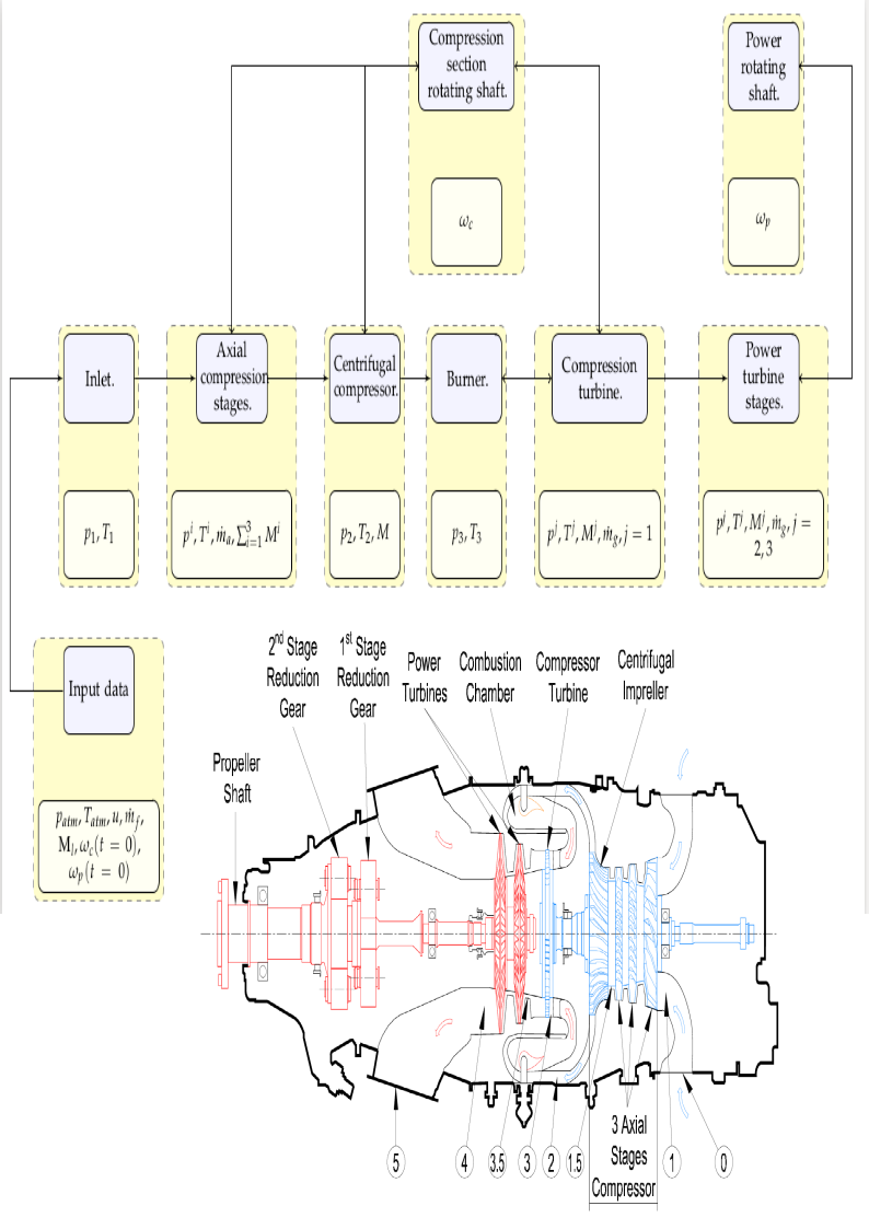
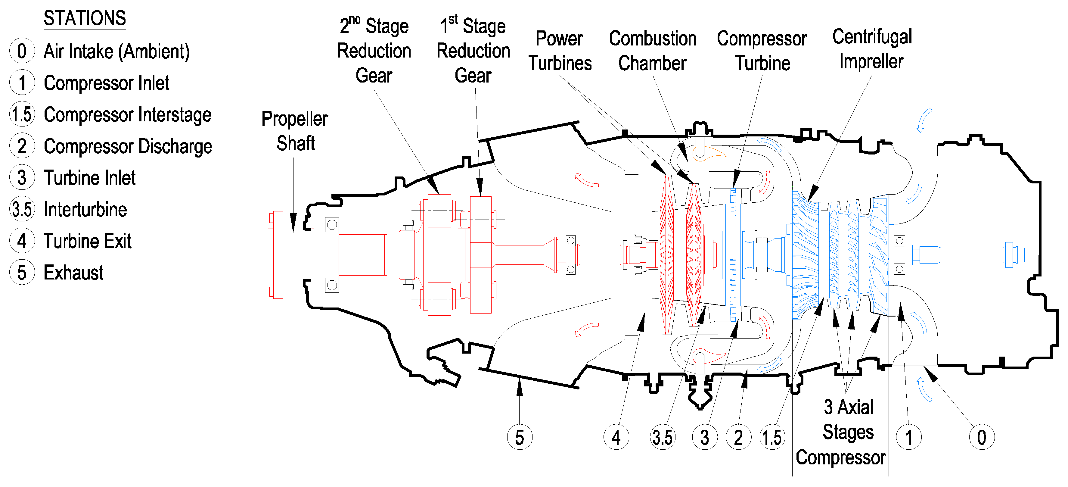
A generic version of the Pratt-Whitney PT6A-65 “Medium” engine, including the labeling of its parts, is displayed in
Figure 1. In general, gas turbine engines consist of: an air inlet, a compression section (including the compressor and diffuser), a combustion section (combustion chamber), a turbine section, an exhaust section and an accessory section (for necessary systems). The theoretical description of the thermodynamic processes occurring in these components is Brayton’s cycle. But the dynamic simulation of the engine’s behavior must account for non-equilibrium conditions, which is the case of the start-up procedure of the engine. The Brayton’s model must, therefore, be complemented with the actual design of the turbo-machinery of the engine’s stages.
We develop a gas-dynamical model for describing the thermo-fluidic phenomena present in each gas turbine engine’s component. For doing so, we apply the fluid’s continuity balance for every component of the engine. Especially those with transient mass storage, namely the combustion chamber where compressible effects of the air are relevant and for the coupling of mass fluxes between consecutive components. We also apply the fluid’s momentum balance at the core flows in the compressor and turbine stages. Fluid’s energy balance accounts for the combustion chamber heat addition and the compression and expansion processes. The mechanical energy equation is also applied to the rotor stages, including the inertial and frictional loses terms of the rotor shaft, to model the mechanical coupling between the moving components. Since our model focus on describing the primary flow-path components and avoids the description of the structural behavior of the solid parts of the engine—which are not essential in the engine’s operation. We also neglect the heat transfer between the solid metal components and the gas in the energy balance equation. As reported in previous works such as Ref. [
18], some other non-flow-path components affect the ability to maintain the operation conditions and accounting for them can be significant to obtain accurate simulations. This is the case of the combustion model, the fuel system or the external loads related to the propeller. Although we acknowledge the importance of these systems, we exclude the engine-inlet or engine-outlet integration (to reproduce the inlet and outlet flows), the engine-aircraft integration (to reproduce structural analysis), the engine-environment integration (for adverse weather and pollution) and those control systems.
The application of the balances to the engine’s components results in a 0-dimensional model representing the operation at transient state. This “aero-thermal” model is usually confined to the normal operating range of the engine but in the present work it is aimed at giving the engine response at off-design operating conditions. A practical approach to numerically solving the 0-dimensional model is to implement it in Matlab-Simulink
® software [
28], which possess a graphical user interface for building algebraic block diagrams that give solution to the governing differential equations. Hence, we present the global block diagram of the governing equations in
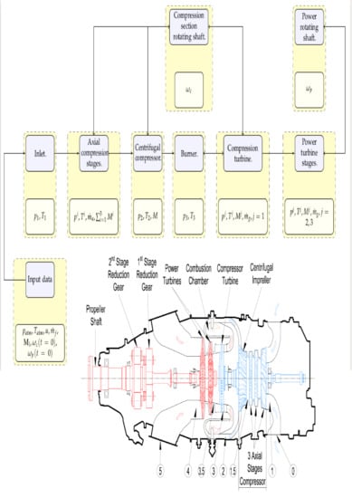
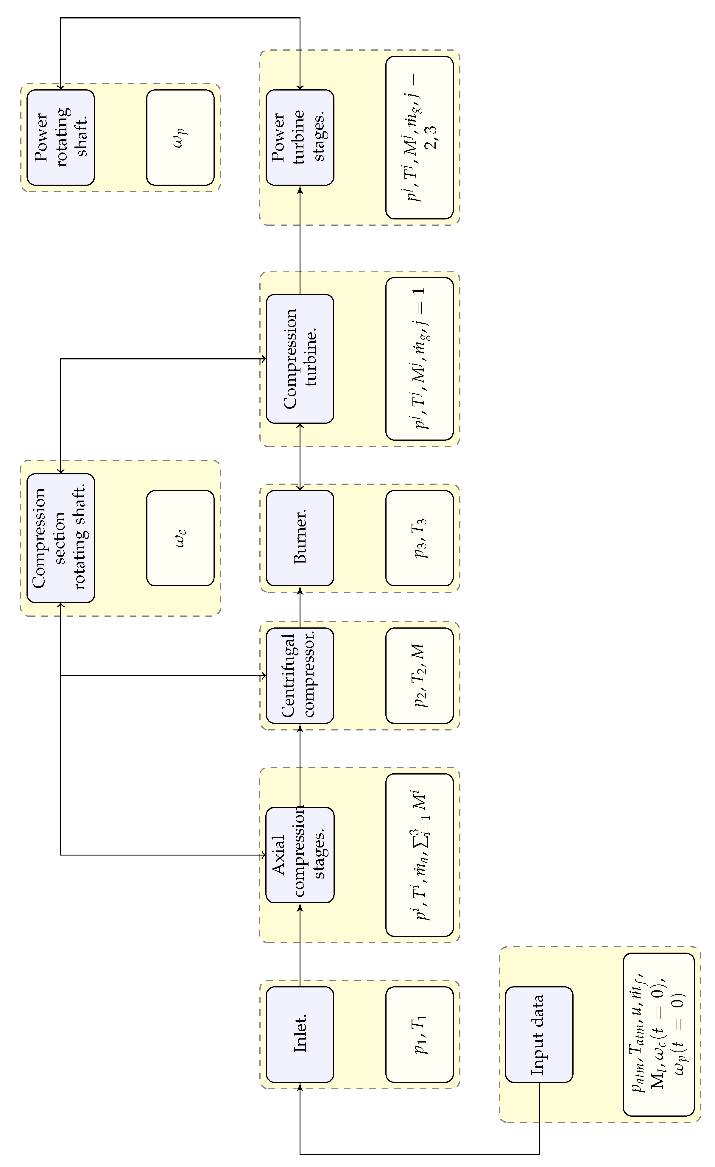
Figure 2, where the engine model is represented at a component level. An extended explanation of each engine’s component and how we represent it, will be developed through the following paragraphs. Moreover, each component’s block diagram will be presented through the detailed explanation of each sub-system. We list inputs, parameters, variables and outputs for every block diagram.
2.1. Air Inlet
One of the main characteristics of this gas turbine engine is that it is mounted backward in the nacelle in most aircraft installations. This feature makes that the airflow is directed inside the components of the engine in the same direction as the aircraft’s displacement. Another consequence is that the intake is located at the rear part of the engine and therefore, the air passes through the exterior of the aircraft (and the engine itself) before entering to the intake. The PT6A-65 design cares for guiding the intake air to the engine using ducts that avoid facing the exhaust gases: since the typical requirement is to provide laminar and clean air into the compressor—so that, it can operate at maximum efficiency—, the inlet duct changes smoothly from opposing the direction of the airflow to the axially forward direction of the aircraft’s speed.
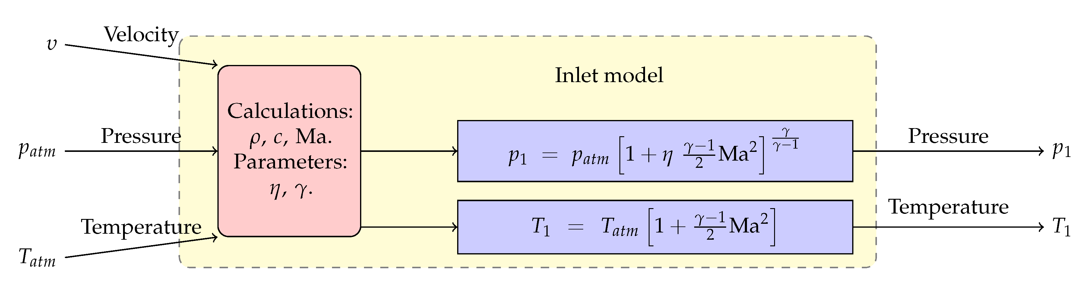
We define the inlet component as to be the intake air conditioner: even though our model is restricted to an on-ground operation, with no rarefying processes of the atmospheric air entering into the engine, we extend the possibility of the operation of the model during in-flight operation conditions. This effect is modeled using the relations for the pressure and temperature of the air which are presented in the block diagram of
Figure 3. In the model,
and
are the atmospheric pressure and temperature, Ma
is the flight Mach number that relates the aircraft speed
with the speed of sound
. The quotient between specific heats of the air is denoted by
and
is the polytropic efficiency. We use the subscript 1 to label the thermodynamic variables of air at the inlet. Note that when the engine is supposed to operate in the ground test bench, the model equates the inlet conditions to the atmospheric conditions
and
.
2.2. Compression Section
The compression section of the PT6A-65 gas turbine engine (used for aviation) consists of three axial stages and a single centrifugal stage, each considered to be a rise in the air’s pressure: the air flows from the inlet duct to the low-pressure compressor and then to the next two axial-flow stages before passing to the centrifugal stage. The axial stages are composed by rotating blades called rotors and static blades called stators. Those rotating stages move at around 40,000 Revolutions Per Minute (RPM) increasing the air’s pressure more than eight times the inlet’s pressure. The last stage of the compressor section is composed of a single centrifugal-flow compressor that accelerates the air outwardly. This centrifugal section has a high-pressure rise but since there can be several losses between centrifugal stages, it is restricted to a single-stage before discharging the airflow. The air stream then leaves the centrifugal compressor section via the diffuser, which is a section of the engine just before the combustion chamber that has the function of preparing the air for the burning area so that it can burn uniformly and continuously. We neglect the diffuser in our representation of the compression section of the engine.
Preliminary work to the modeling of the compressor has to do with the estimation of its geometry. In this sense, we determine the compressor’s geometry by extracting most of the information from technical reports, as well as from the engine’s manual [
29]. Since the axial compression section geometry has been reported in Ref. [
30] for a four-axial stages PT6A-65 engine, we transcript the geometrical parameters for the first and last stages but calculate the mean values of the second and third stages of that compressor and set those values as the second axial stage of our PT6A-65 axial compressor model. The geometric parameters that we have processed for each axial stage geometry are presented in
Table 1. In the case of the inner and external radius of the rotor blades, we determine those parameters from cross-checking the engine’s manual schemes and the measured values from a disassembled engine. The geometry model of the centrifugal compressor is completely defined with the rotor’s blade geometry and the inlet’s and outlet’s cross-sectional dimensions. Where the inner
and outer
radio of the rotor are determined from the engine’s technical report, being 92 mm and 117 mm, respectively.
The overall compression stage is defined from the compressor intake to state 2, at the diffuser outlet . Therefore, it spans the three axial stages, the centrifugal stage and the diffuser of the PT6A-65 engine. In the present approach, we formulate the mass, momentum and energy balance equations over each sub-stage of the compressor to create a physically-detailed model. Knowledge of the inlet (upwind) conditions of the air, such as temperature and pressure, as well as the rotational speed of the engine’s rotating shaft, are required. We also demand the knowledge of the geometry of the compressor at each stage: since each compression section is composed of successive stages of rotating blades (rotors) and stationary guide vanes (stators), we analyze at each rotor-stator stage the transmission of the shaft’s mechanical energy into the air’s fluid energy and compose the complete compressor performance by adding the multiple successive compression stages.
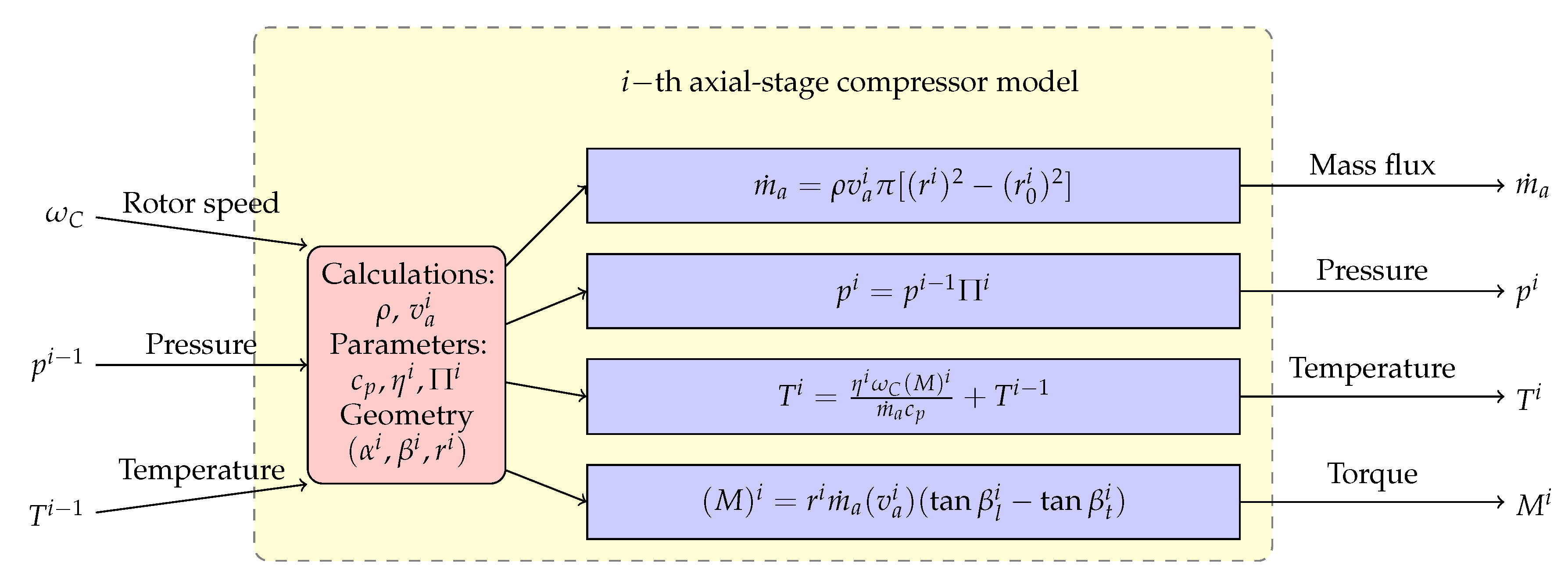
For simplicity, we assume that the compressor’s blades are thin, rather than having the complete airfoil cross-shape geometry. This supposition is acceptable since in the PT6A-65 engine those are constructed of sheet metal. In the case of the axial compressor, we analyze a single th stage, where a rotor precedes a stator and consider the same hub radius for the rotor as for the stator. We also make this supposition for the shaft radius at each axial stage. Nevertheless, we consider different cross areas between consecutive compression stages, such that the axial component of velocity can be calculated to conserve mass: in the case of the multistage axial-flow compressor, the blades of each successive stage of the compressor get smaller as the air gets further compressed. In each rotor-stator stage, we consider the cross-section of only one stator and rotor blade as it moves vertically, knowing that the next rotor blade passes shortly thereafter. This is the well-known cascade two-dimensional approximation of turbomachinery analysis and which configures our control volume.
We aim to calculate the variation in the air’s enthalpy originated by the rotor’s torque. To do this, we apply a simplified analysis of the fluid’s dynamics of the air occurring through the blade: the
velocity triangle. With this approach, no component map representations or error relationships for the guesses of the unknowns are required and therefore, no convergence issues of the numerical solution are found. Instead, direct physical solutions are encountered for each component with the corresponding avoidance of convergence problems. To do this, the axial speed of the airflow
can be measured at the inlet section, such that the volume flow rate can be calculated in terms of the cross-sectional area. Another possibility is to know the inlet air angle (presented in
Table 1), such that the axial velocity is calculated from the velocity triangle. To evaluate the torque on the rotating shaft, we use the angular momentum balance that states that the total momentum in the shaft
is equal to the change between the angular momentum of the flow that crosses the surfaces of the control volume. This change is only related to the tangential velocities of the air given by the velocity triangle analysis.
In our model, we consider irreversible losses in the compression stages and therefore, we include an irreversible mechanical efficiency
that implies a gap between the shaft power and the power delivered to the air. We suppose a quasi-static and polytropic process in which the increment of energy in the air is given by the addition of mechanical power. Indeed, the temperature rise inside the axial compression stage is calculated by applying the energy balance in the control volume. The pressure ratio
(or net pressure head) induced by the compressor is calculated with the polytropic process relation knowing the temperature variation of the air and the polytropic constant of the gas
n. The previous exposition is demonstrated in the block diagrams of
Figure 4 and
Figure 5.
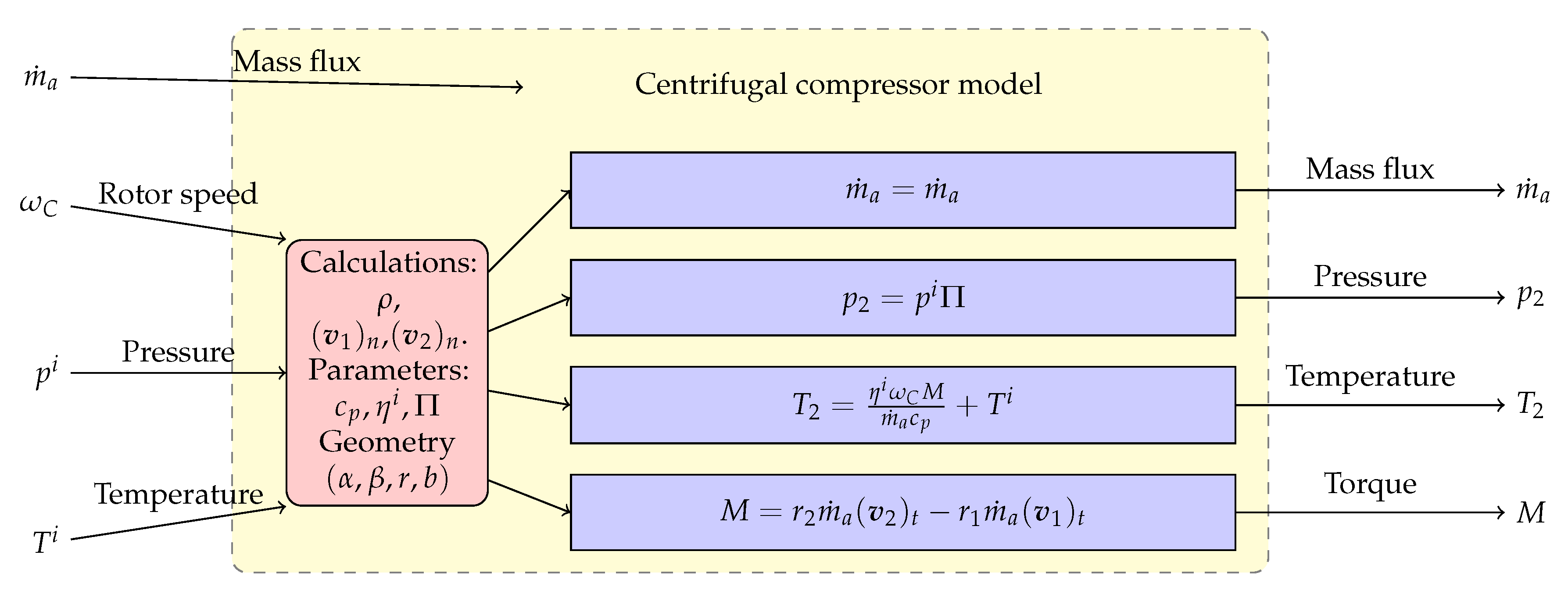
For the centrifugal compressor, we consider that the circumferential cross-sectional area can be defined by the radius and the width of the blade b. We also suppose that the flow is defined completely in the normal direction and therefore, the normal velocity at the outlet of the blade can be calculated with the conservation of mass.
2.3. Burner
The PT6A-65 burner is mainly characterized by the split in the amount of compressed air that is used for maintaining the combustion: only a fraction of the air entering in the burner reacts with the fuel, while most of the compressed air is used for cooling purposes. The geometrical shape of the burner chamber is an annulus. In this sense, the overall volume is hard to be determined and we have approximated its value from measurements of the disassembled engine’s burner to be around m.
Inside the burner, the fuel and the air are separated apart before the flame: combustion with the liquid fuel is performed by the injection of the fuel inside the air stream. Scattering of the fluid into fine droplets leads to the convection and final evaporation of the liquid inside the compressed air-stream. This mixture is a steady non-premixed stream of air-fuel before the full combustion reaction takes place inside the burner. Buoyant mechanisms but mostly forced convection and turbulence mechanisms of inlet air (due to its high pressure and temperature at the exit of the compression section) maintain the combustion process in the flame. The reaction rate and the products of the combustion (exhaust gases) depend on the quality of the air-fuel mixture occurring before the flame.
The combustion quality is automatically controlled by the fuel control system that fixes the amount of injection; this control is set by default for the Jet-A1 fuel. We neglect the fuel control in our present approach since we aim to investigate the response of the engine to different blends with biodiesel. The change in the physical properties of the fuel affects its spraying as it passes through the fuel injectors in the combustion chamber. This has effects on the maximum temperature inside the fuel chamber at the start-up of the engine. In this sense, the starting procedure has to be designed to be rigorous and must be established for each new operating fuel. For all the above, computational simulation of the particular gas turbine engine’s performance is proposed as a predictive tool for the engine operation, which allows determining the operation variables when the change in the composition of the fuel occurs. This, with a low cost and without risking the operation of test engines.
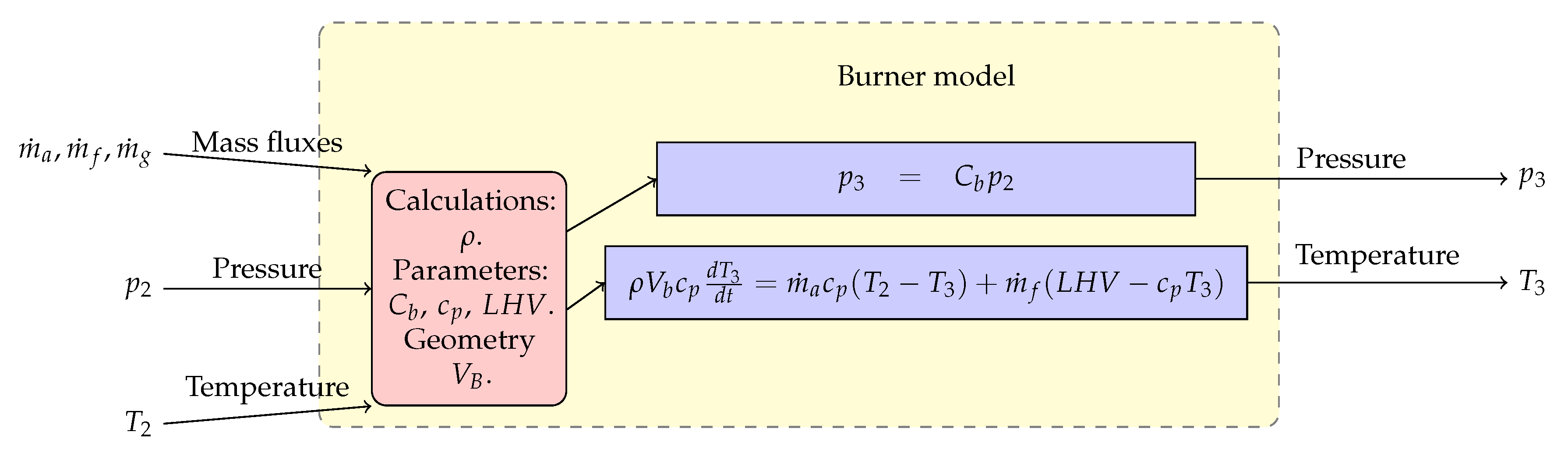
Our approach to model the burner’s combustion phenomena is simple and follows previous approaches like Ref. [
27]. The net power of the gas turbine engine is related to the amount of fuel that is burned inside the burner—the heat added to the air-stream is calculated from the energy balance inside the burning chamber, where
is the Low Heating Value of the fuel that represents the amount of energy that is delivered in the combustion process (accounting for the steam boiling in the liquid fuel). This is depicted in the block diagram of
Figure 6.
Note that the amount of chemical energy that is transferred to the air (which is later transformed to mechanical energy in the turbine) depends on the type of fuel used and this is completely characterized by the fuel flow rate and its lower heating value. The burner also works as an accumulator of mass, where the temporal change of the thermodynamic conditions of the air inside the burner is related to the amount of fuel
, the incoming airflow rate
, the exhausting rate flow of gasses
and the volume of the chamber
. Note that the fuel flow is the input specification for the fuel burner model, not the Fuel-to-Air Ratio (FAR) or the combustion temperature. The pressure drop across the burner has also been adopted from Ref. [
27], with the loss coefficient
, depending on the square mass flow rate.
2.4. Turbine Section
The air stream leaves the burner with the addition of heat from the combustion and flows through several turbine stages. The first turbine stage is a single-stage axial turbine that powers the compression section synchronously rotating at 40,000 RPM via the engine spool or common shaft. From measurements of the disassembled engine spool, we determine an overall mass moment of inertia of the engine spool of about kg m.
In the PT6A-65, the hot air flows then into the power turbines, which are composed by two axial stages that turn at about RPM and that are connected to the main shaft that drives the propeller (or load). We also determine that the mass moment of inertia of the main shaft is kg m. The air is discharged next to the exhaust and then to the atmosphere, where the air recovers its original free-stream conditions.
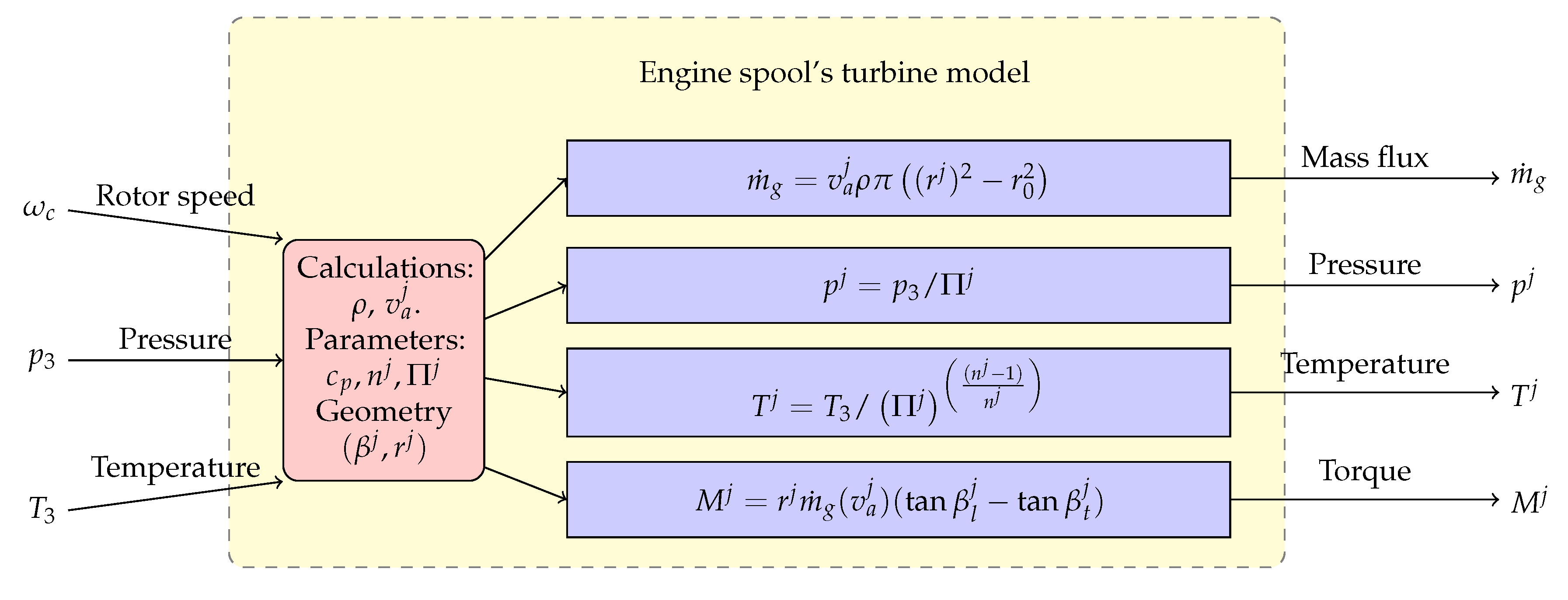
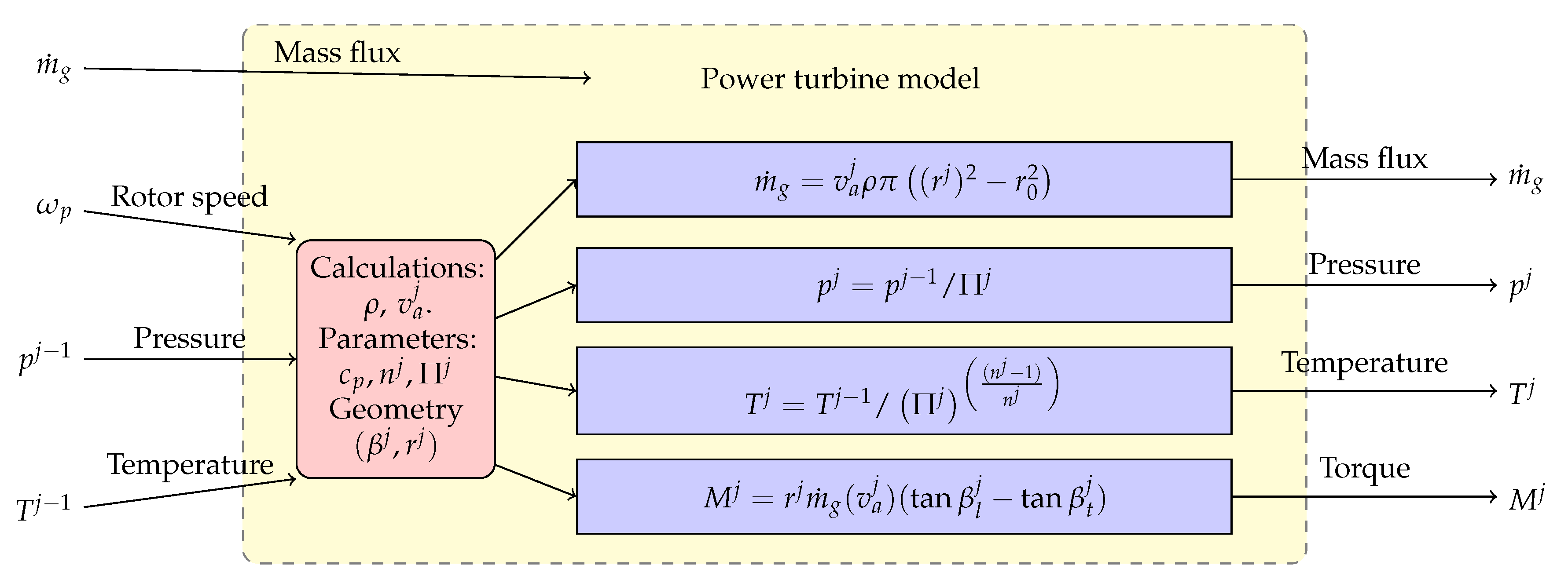
The turbine process is defined from the state 3 at the combustion chamber outlet to state 4, at the engine outlet . This means that the expansion ratio of the gas is known for the turbine section. Indeed, knowing the expansion ratio of the th stage, one can model each turbine stage as a polytropic expansion process where the pressure and temperature of the air at the discharge can be calculated straightforwardly.
The temperature drop is then used to calculate the retrieved mechanical power inside the turbine. Again, we suppose an irreversible process efficiency between the fluidic and the mechanical power, such that the extracted torque at each axial stage of the turbine differs from the change in the angular momentum of the air inside the turbine. Similarly to the axial flow compressor analysis, an accurate model of the turbine performance can be derived from a detailed computation of the aerodynamics of the flow over the individual blade elements. The distinctive feature of the turbine is that the mass flow rate of gases through the turbine section depends on the expansion work: we use the angular momentum balance to obtain the mass flow of gases through the turbine stage and therefore, the axial term of the air velocity. The turbine relations are presented in the block diagrams of
Figure 7 and
Figure 8.
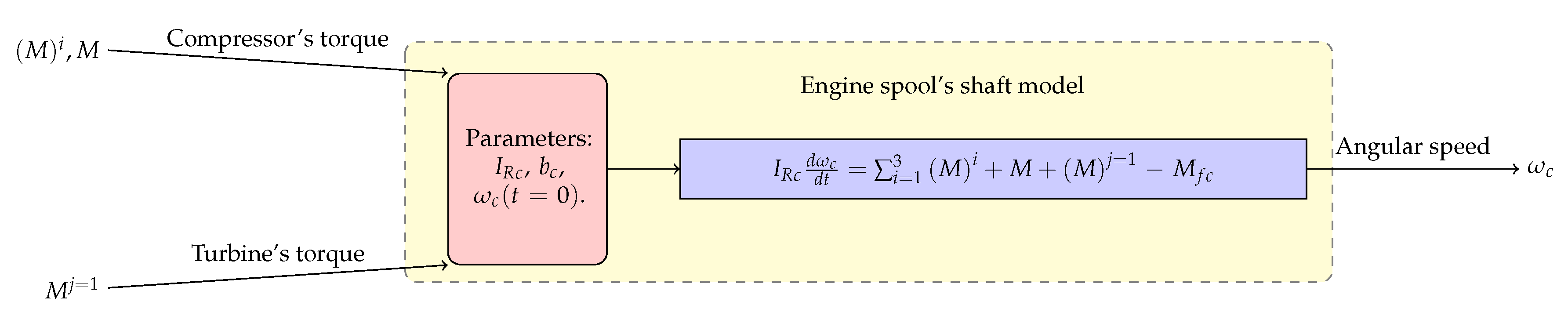
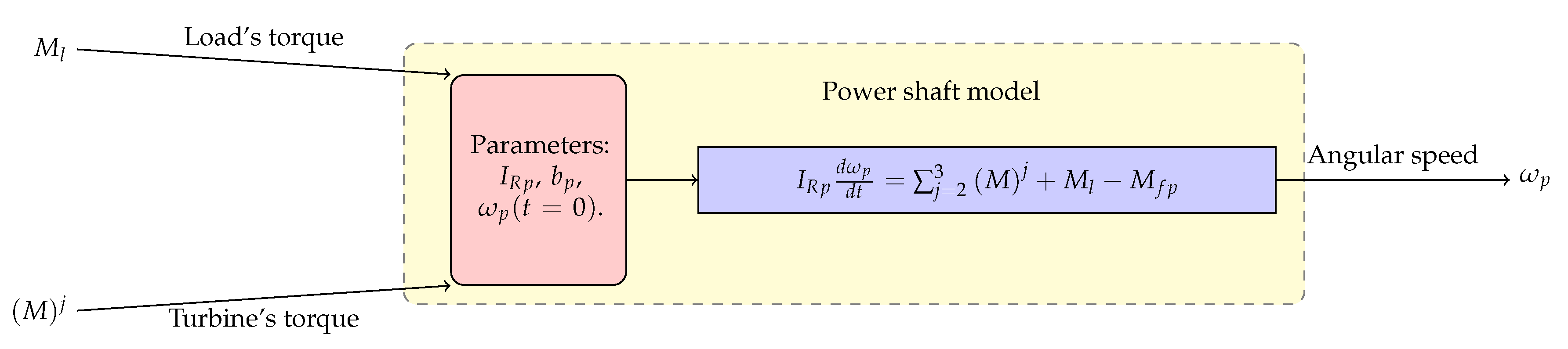
2.5. Rotating Shafts
The rotating shafts are modeled by applying the balance of angular momentum. We use the rigid body assumption and apply the momentum balance in the rotational motion, such that the acceleration power of the shaft must equal the balance between turbine power, compression (or load) power and parasitic powers. The angular momentum balance applied to the engine spool, as well as the power rotating shaft are presented in the block diagrams of
Figure 9 and
Figure 10, respectively. We define
to be the mass moment of inertia of the rotating shaft about its rotating axis,
is each one of the torques applied to the shaft and
is the angular velocity of the shaft which can be calculated in terms of
, being
N the revolutions per minute. The sum of power losses due to mechanical friction is considered in the torque
, which is modeled using a loss-factor
b that is a function of the rotational speed of the shaft and its effect acting in the contrary-rotation sense. Following Ref. [
27], we apply this mechanical losses model instead of including a mechanical efficiency parameter of the shaft. This is explained since the numerical accuracy of the model can be granted at the idle condition and during the start-up procedure when the output power is negligible.
2.6. Compatibility Conditions
Besides the physical description of each engine’s component, one must close the engine’s model coupling the different components to what is referred to the
compatibility conditions. The overall compatibility conditions become clear from the engine system’s block diagram depicted in
Figure 2.
The mass compatibility conditions are related to the conservation of the air mass flow rate. The inlet’s air mass flow rate is calculated by knowing the inlet air angle at the first axial stage, such that the axial velocity can be calculated knowing the rotational speed and the geometric parameters of the rotor blades. It has been explained that is conserved among the stages of the compression section. Nevertheless, the mass compatibility condition differs substantially when the air enters the burner: the exhaust gasses mass flow rate is not only related to the compressed air flow reacting with the mass flow of fuel but the exhaust gasses depend on the flow through the turbine section and the engine’s exhaust. Here the compatibility condition is related to the mass flow rate resulting from each turbine stage. Some further explanation about this compatibility condition will be taken in the next section.
On the other hand, the angular momentum compatibility condition is the balance of the torques applied for each rotating shaft. Its readily understood that the rotation speed of the axial and centrifugal compressor stages matches with the compressor’s turbine via the engine spool. In the same line, the velocity of the power turbines rotating shaft matches the propeller’s shaft velocity through the reduction gear.
Finally, the energetic compatibility conditions are associated with the thermodynamic variables of the air at each one of the stages of the engine. It has been readily mentioned that the air enters each consecutive stage with the pressure and temperature conditions that it obtains at the stage immediately before.
3. Numerical Results
In this section, we present the numerical results for several simulation scenarios. As explained before, the numerical solution of the set of algebraic and ordinary differential equations is achieved by Matlab-Simulink
®. A fourth-order Runge-Kutta numerical scheme for the temporal integration is used for solving the differential equations. A maximum integration step of 1ms is used to guarantee the stability of the temporal solution. The first scenario is the steady response of the engine which is intended to validate the computational model. Two models are set up, one with the present approach and the other one using GasTurb
® [
23]. We test both models to ensure the accuracy of the developed model at steady-state operation conditions, and to validate our results with the engine test data and the commercial software simulation. Then, we solve the steady-state operation by using the blends with biodiesel and compare our numerical results with the ones obtained with GasTurb. Finally, we address the transient operation of the engine using the fuel blends, specifically at the start-up of the engine when the maximum temperature can be reached. We suppose in all scenarios an on-ground operation so that the inlet velocity is zero.
3.1. Validation of the Computational Model
We first validate the computational model by considering the standard operation of the PT6A-65 engine reported in the operation manual [
29]. Those operation parameters are presented in
Table 2, where the International Standard Atmosphere (ISA) conditions are set as the environmental conditions. We evaluate the stationary response of some tracked variables (invariant in time): for the sake of validation, we track the stationary pressure, temperature and airflow at the stations of the engine. In
Table 3 we list the experimental results that have been reported in the operation manual for several stations of the engine, and that we use for the sake of comparisons.
Correspondingly with
Section 2, the geometrical parameters of the PT6A-65 motor described in that chapter are implemented in our computational model. We fit some remaining geometric parameters so that we obtain the closest numerical results to the ones reported in the operation manual: first, we determine the compression and expansion ratios based on the experimental measurements. The overall compression ratio at the axial stages can be calculated from the data in
Table 3 to be 3.14:1 atm, while for the centrifugal compressor the compression ratio is around 2.56:1 atm. In this sense, we fit the centrifugal compressor’s angles
and
to 40 and 38 degrees, respectively, such that the centrifugal compressor gives rise to the pressure change. On the other hand, the expansion ratio for the compression and power turbines are calculated to be 1:3.03 atm and 1:2.18 atm, respectively. We suppose an expansion ratio of 1:1.47 atm for each stage of the power turbines section and fit the blade’s angles to fulfill the mass flow rate compatibility (conservation) condition between the different turbine stages.
Another quantity that the computational model requires is the
n polytropic index for each compression and expansion stage. We calculate that index by solving the logarithmic inverse expression for a polytropic process and accounting for the experimental PT6 engine operation. This is, considering the data in
Table 3, one can obtain the polytropic index with the expression
Subscripts
i and
f of the previous relation denote the initial and final condition of the gas in the polytropic process, respectively. Then, the irreversible efficiency
of each compression and expansion stage can be computed from
, where the
value corresponds to the air (not to be confused with the overall engine’s efficiency). The gathered polytropic indexes and irreversible efficiencies for the compression and expansion sections of the PT6A-65 engine are presented in
Table 4. Those values are set in the energy balances and polytropic processes of the compressor and turbine stages.
Table 5 presents the fitted aerodynamic and geometric parameters for all the turbine stages of the PT6A-65 engine that required to be processed. These parameters are determined following the previously exposed ideas, from cross-checking the engine’s manual schemes and the measured values from a disassembled engine but mostly from the fulfillment of the mass conservation requirement. The rotor blade airfoils, which are metal profiles followed and preceded by stator vanes, are completely defined by these geometric parameters. Finally, the parasitic power that is lost due to friction can be modeled by setting the bearing coefficients
and
to
kg·m
/s and
kg·m
/s, respectively, for the engine spool and power rotor shaft. We also model the pressure loss coefficient in the burner to be
. These values arise from the numerical experiments that we performed guaranteeing the best approximation of the computational model to the referenced values of the engine’s steady operation.
The simulated steady engine response is presented in
Table 6. In those results, we have assumed a constant flow of Jet-A1 fuel, with a calorific power of
MJ/kg and a constant propeller’s load torque of
N·m. We confirm a consistent physical behavior of the thermodynamic variables with the experimental reported ones. Distinctively, the observed pressure at the discharge of the axial compressor stages is higher than the reported one. This inaccuracy is countered by the centrifugal compression section, where the blade’s geometrical parameters are fitted to give accurate results of the overall compression ratio. In this regard, fitting the compressor’s parameters affects negatively the accuracy of the temperature at the discharge of the compression stage but the energy balance inside the combustion chamber counteracts this effect and matches the stipulated temperature in the manual, with an error of only 1.57%.
Temperature and pressure variables at the expansion stages correspond well to the experimental counterparts, mainly due to the possibility of fixing the expansion relation and the geometrical parameters of the turbines. Given the previous exposition, we believe that the error is restricted to a low range such that it validates the usage of the proposed model for predicting the engine response when new operating conditions are evaluated.
As explained before, we also implement the PT6 engine in the GasTurb software to validate our results: we simulate the stationary operation of the engine using the Jet-A1 fuel and the same operating conditions that have been listed in
Table 2. Since the GasTurb software has three different simulation levels: the basic thermodynamic approach, an engine’s performance mode and a more advanced engine’s performance simulation that considers the specific geometry of the gas turbine engine, we choose the engine’s performance simulation. We select the default two-spools turboprop template that includes a booster and a compressor, the combustion chamber and the two expansion stations but modify the template by including a high-pressure turbine in the engine’s spool and a low-pressure turbine in the power spool. The inputs for simulation in GasTurb are also the polytropic efficiencies of compressors and turbines, the atmospheric condition (temperature and pressure), the drop pressure in the combustion chamber, the low heat value of the fuel, the maximum temperature in the combustion chamber and the pressure ratios in the compressor and turbine stations. The temperature and pressure results along the stations of the PT6A-65 engine, together with the calculated relative error against the experimental measurements are presented in
Table 6. The comparisons between the developed model results and GasTurb demonstrate that although there are some errors for certain stages in each model, the results from the present approach do not differ in accuracy than those given by GasTurb. These results guarantee an acceptable resolution of the present approach and give the certainty to apply it in the PT6A engine evaluation when operating at off-design conditions.
3.2. Stationary Operation of the PT6A-65 Using Fuel Blends
Once the present computational model has been validated, the following simulation scenarios are considered: we evaluate the stationary operation of the PT6A-65 engine at both 100% of the fuel mass flow and 60% of the fuel flow, meaning full throttle and idle operation, respectively. Since we aim to predict the engine’s response to the usage of new hypothetical fuels, we vary the parameters related to the fuel’s modeling. In this sense, the standard Jet-A1 fuel—kerosene—is mainly composed of
heptane and isooctane, which are hydrocarbons that possess between 8 and 16 carbon atoms per molecule, giving a
of around
MJ/kg (measured in experimental tests [
31]). On the other hand, the chemical composition of a biodiesel sample has been measured in Ref. [
32] giving an approximated
value of
MJ/kg. Hence, the pure biodiesel retains a smaller amount of energy than conventional Jet-A1 fuel.
We simulate the engine operation with hypothetical blends of Jet-A1 with biodiesel. These fuel blends are abbreviated as KB#, where “K” represents the Jet-A1 as the primary fuel, “B” represents the biodiesel as the secondary fuel and # is the mass fraction of biodiesel in the blend expressed in percentage. We establish a discrete range of mass concentrations of biodiesel in Jet-A1 which are 3 in total: KB10, KB20 and KB30 and calculate their
using the percent by mass of the mixture. The KB0 and KB100 represent the pure Jet-A1 and pure biodiesel fuels, respectively. In the successive, we plot the simulation results for the operation with different blends of fuel, so that they are easily comparable.
Table 7 shows the
for each blend and the notation to be used in the plots.
Figure 11 shows the air pressure through the engine stages. We observe a pressure rise at the compression section, as well as an expansion process at the turbine stages. It is evident for both throttle operations that the maximum pressure is located at the centrifugal compressor’s discharge (stage 2) and that there is a slight loss in this pressure at the burner (stage 3). In the full-throttle case (right side of the figure), it can be observed that the pressure gap between the Jet-A1 fuel and the pure biodiesel fuel is considerable, with an observable maximum pressure of 750 kPa and a lower pressure of 610 kPa. In the case of the idle operation, there is a difference of 60 kPa between those fuels, with a maximum pressure of 460 kPa and a minimum pressure of approximately 400 kPa. The fuel blends give results that lay below some
of the Jet-A1 pressure range. In any case, the maximum values of pressure are related to the use of the Jet-A1 fuel. This can be explained since it delivers the highest amount of power, which in turn is extracted by the turbine stage and transferred to the compression section via the engine spool.
Figure 12 displays the air temperature through the engine stages for the two different throttles. The temperature results agree well with those reported in the manual: the maximum air temperature is observed at the burner discharge (stage 3). In any scenario, the fuel that provides the highest temperature to the engine is the Jet-A1 fuel. For the full-throttle operation there is a 200 K temperature difference in the burner between the Jet-A1 fuel and the pure biodiesel fuel: the maximum temperature is given for the Jet-A1 fuel, reaching 1290 K, while the minimum temperature of 1104 K is given by the biodiesel operation. The highest drop in temperature occurs at the compression turbine, while the power turbines contribute lesser to the temperature reduction. It is also observed that the temperature difference arising between the fuels at the burner is kept constant at the turbines discharge (stage 4). No important temperature variation is observed for the biodiesel blends. Regardless of the fuel type, the temperature never exceeds a value of 1050 K for the idle operation.
We also use GasTurb software to evaluate the engine performance running with biodiesel blends. Hence, we display in
Figure 13 the pressure and temperature results obtained with the GasTurb model for the full-throttle operation. We can observe that the GasTurb results for the different mixtures do not vary significantly. Although we have imposed modified LHV values for each fuel, the GasTurb model seems not to be sensitive to these variations. On the contrary, in our results, we can appreciate the variations in pressure and temperature that were commented previously.
3.3. Transient Operation of the PT6A-65 Motor Using Fuel Blends
Finally, we evaluate the start-up procedure of the engine with the fuel types that have been tested in previous scenarios. The main goal is to identify problematic conditions during the engine start-up, which is the transient procedure that can actually affect the engine’s integrity. The model is intended to run at zero speed and sea level conditions, since the off-design operation of the engine are evaluated on a test bench. Being a two-spool turboprop, the PT6A engine has been designed to be electrically started. The starter motor is represented in the engine simulation as a constant rotational speed and starter torque. Hence, at the start up process, a simplified model with the imposition of the rotational speed at the compression shaft and a constant torque load is implemented. The simulation is also intended to run from idle to maximum power but no shut down simulation is proposed since the objective is focused on the combustion chamber’s limits. We configure the start-up procedure such that the compressor’s shaft starts accelerating from its steady state condition to 12,000 RPM, which is the rotational speed that is provided by the starter. From this point, there is a positive increment of the air pressure (given by the rotation of the compression system) until the desired mass flow of air into the burner is granted. During the initial compression operation, no fuel mass flow is injected into the burner. We consider that at a later instant s, when the compressed air into the burner stabilizes, the fuel is injected into the burner and ignited. The mass fuel flow is then gradually increased until the desired throttle is reached at . All the start-up procedure is considered to undergo with a constant torque at the propeller’s shaft N·m.
We aim to evaluate the start-up procedure of the PT6A-65 engine with both 100% and 60% of throttle. The results for the operation with fuel blends are displayed similarly as for the stationary operation. We present comparisons of some important variables, such as the air pressure at the compressor discharge and the air temperature inside the burner. It is noticeable that the start-up procedure converges to the steady-state operation.
Figure 14 shows the transient pressure results at the compression stage for the two different throttles. It can be observed that the pressure in the compressor’s discharge undergoes an initial equilibrium when the engine spool is started, reaching a compression ratio below of 1.5:1 atm. At
s, when the fuel is ignited, a sudden increment of the compression ratio of around 2:1 atm is noticed for all fuels and throttles. In the case of the
throttle, the pressure stabilizes from this instantaneous peak but a pressure increasing delay for the full throttle case is noticeable, reaching lately the reported 8:1 atm compression ratio. There is not a significant pressure fluctuation related to the fuel blends: it can only be appreciated a moderate increment for the full throttle and the biodiesel fuel than for the blends and Jet-A1 fuel.
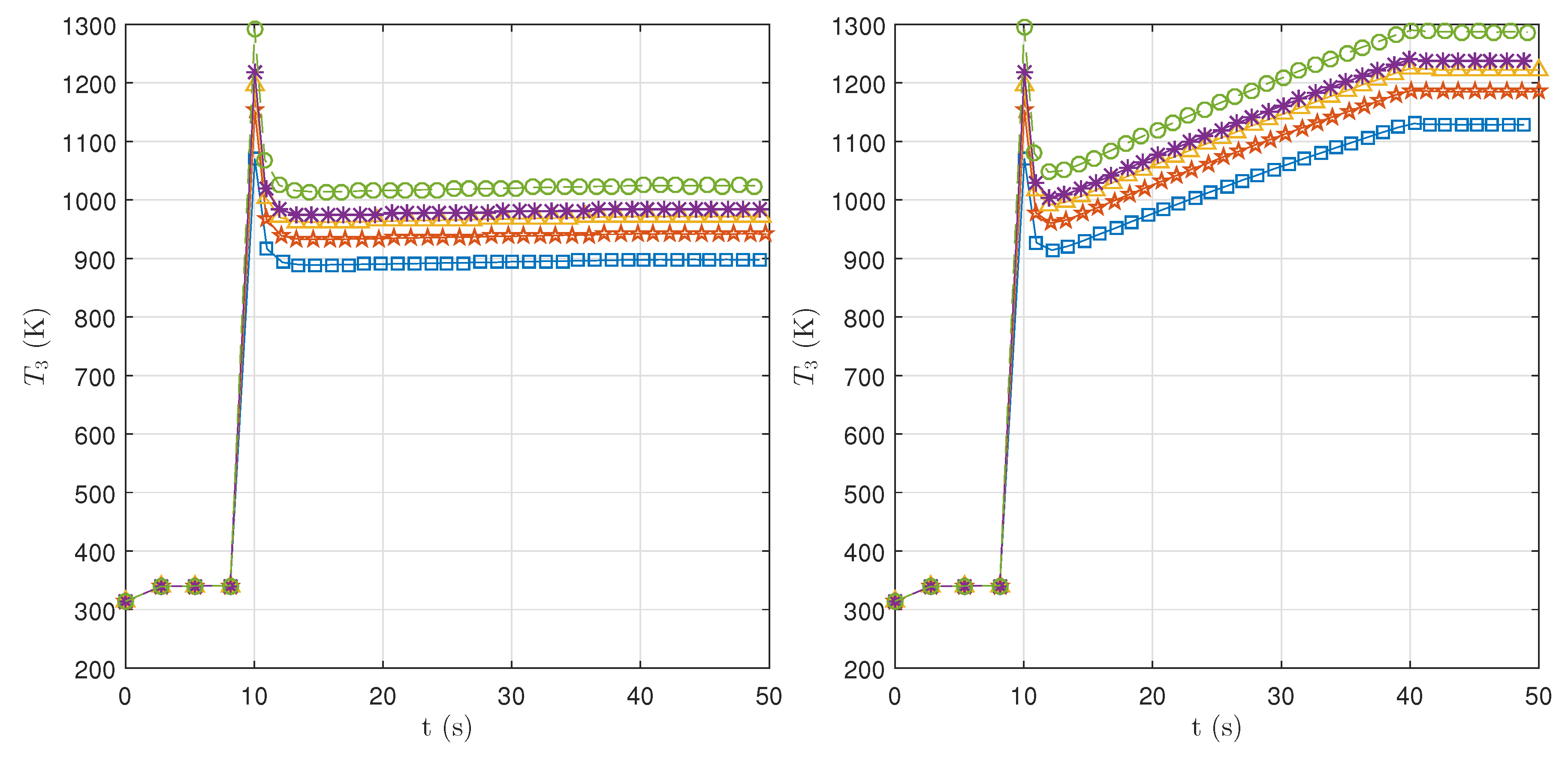
The transient temperature inside the burner is presented in
Figure 15 for the two different throttles. We observe a slight increment in the temperature at the initial compression operation. Then, the fuel intake generates a temperature peak in the combustion chamber, which in all scenarios is the maximum temperature that is reached during the complete operation of the engine. Since the initial fuel flow is the same for both throttle scenarios, the maximum temperature in the engine does not vary. Instead, it only depends on the fuel blend, where the maximum temperature of 1300 K inside the burner is obtained with the Jet-A1 fuel, and the minimum of around 1100 K, approximately, is obtained with the pure biodiesel. This is explained by the relatively smaller LHV of the biodiesel, which affects the gas turbine combustion. After this critical instant, the temperature stabilizes at around 1000 K for the idle operation, with fluctuation slightly greater than 100 K between the JetA1 and the biodiesel fuel. On the other hand, the temperature in the full-throttle scenario increases gradually until the steady-state of 1290 K is reached at about 40 s.
The first remark up to this point is that temperature controls have not been implemented in the present model. Instead, we want to establish the hypothetical temperature that is reached during the ignition procedure. Using the present computer engine model we can compare the start-up operating temperature against the reference given by the engine test data, which is the limit for structural integrity reasons and shutdown limit. In this sense, the standard 1300 K temperature limit [
29] is not reached by any off-design operational scenario. The tests of the engine operation with biodiesel blends show that the maximum temperature is lesser than 1220 K, which is acceptable for structural reasons of the engine. However, in the real engine operation, the fuel is introduced by the fuel control system. Since the accumulation of unburnt fuel can result in a flammable mixture that can potentially lead to an explosion in the engine, the real combustion with biodiesel blends is controlled by this system. We acknowledge the limitation of not including the fuel system but consider it as future work to expand the present model.
Another remark is that the computational simulations given by Matlab-Simulink agree with the actual physical behavior of the engine, guaranteeing the numerical convergence to the solution at every time step of the transient simulation.
4. Conclusions
In this article, we have developed a functional PT6A-65 engine computer model, which can be used for purposes of testing off-design operating conditions with blends of biodiesel fuel. For this, we have simplified the PT6A-65 engine in a process that extracted the essential components of the engine and eliminated the auxiliary ones. The mass, linear momentum, angular momentum and energy balances have been applied into these components, by which together with the compatibility conditions compose a 0-dimensional aero-thermal model of the engine. We have implemented the numerical solution of the model in the Matlab-Simulink® software and different simulation scenarios have granted the predictive capacity of our computational model concerning the systemic and transient response of the engine. Thus, protecting the actual PT6A-65 plant and incurring in considerable computational advantages like accuracy, economy, expedition and applicability.
Indeed, the achievements of the computer model approach are aligned with our expectations since they have given accurate descriptions of the engine’s performance, not only in the sense that the model has been tuned with the real PT6 operation but also because those are governed by physical expressions. We have obtained the expected performance in terms of desired computational cost. This is one big strength of the present approach, to be able to obtain transitory solutions for the overall engine’s operation in a personal computer. Certainly, this model is a fair trade-off of accuracy/costs since complex CFD models cannot represent the engine’s response in a systematic approach, those can only handle the transient response of very few elements and very limited time ranges.
One general remark is that the dynamical system’s approach (given in algebraic blocks) may be applied to other gas turbine engines: this by modifying the turboprop arrangement with a new connection between the outputs and inputs of the various blocks and without spending too much effort in developing a new computational model. Another is that the present computer model is complimentary to widely used commercial software like GasTurb®. Since the present results and the ones obtained with such software have been compared, we have granted that steady descriptions of the PT6 engine given by our model are at least as accurate and reliable than those by GasTurb®; The relative error between the present results and those reported in the manual is below for most of the stages. But also, that the transient analysis gives a clear advantage to our computational approach.
Concerning the evaluation of the engine’s response to different blends of Biodiesel (or other novel types of fuels), we have obtained the desired predictions: such as the maximum burner’s temperature at the start-up process or the pressure distribution through the engine stages. Regarding the structural integrity of the engine, this approach can give accurate predictions of the temperature in the combustion chamber and evaluate if it remains in the appropriate operating range given by the operation manual (overhaul) such that the operation with the fuel blend does not incur in structural damage of the combustion chamber. The simulation results allow us to conclude that the use of blends of biodiesel that are less energetic than the conventional Jet-A1 fuel would not generate a burner overheating since the standard temperature of 1220 K inside the chamber is never exceeded. It is also clear that fuel blends would not generate a pressure excess in the compressor’s discharge and, consequently, these can not generate internal damage to the motor structure. Those results argue that the proposed methodology can be used in future gas turbine engine’s operation with other fuel blends and the engine’s evaluation in off-design operating conditions.
As future work, kinetic combustion models can be coupled to the present model to determine the added heat and the production of gases. Hence, a natural sequel of the present article is to implement engine control: torque control, pressure control, the fuel system and the combustion control. Even though we recognize that with the present approach we can not calculate the thermal efficiency of the computer model engine since the relation between the engine performance (fuel consumption) against the load is not well represented, we expect to develop a combustion model or a combustion control in our computer model that gives accurate responses of the engine’s efficiency regarding each fuel consumption. We believe that such a work deserves an article on its own and it is not the motivation of the present study. In this sense, reported higher efficiencies for gas turbines operating with fuel blends in References [
25,
26], together with our simulation results, drive to continue working on these topics. Also, non-linear brake models stand as other possible development towards the depiction of the real loading conditions of the engine.

 ,
, 


