Data-Driven Compartmental Modeling Method for Harmonic Analysis—A Study of the Electric Arc Furnace


1
College of Electrical Engineering and Automation, Fuzhou University, Fuzhou 350108, China
2
Fujian Smart Electrical Engineering Technology Research Center, Fuzhou 350108, China
*
Author to whom correspondence should be addressed.
Energies 2019, 12(22), 4378; https://doi.org/10.3390/en12224378
Submission received: 13 October 2019
/
Revised: 6 November 2019
/
Accepted: 15 November 2019
/
Published: 17 November 2019
(This article belongs to the Special Issue Power Quality: Monitoring, Mitigation, and New Types of Disturbances)
Abstract
:The electric arc furnace (EAF) contributes to almost one-third of the global iron and steel industry, and its harmonic pollution has drawn attention. An accurate EAF harmonic model is essential to evaluate the harmonic pollution of EAF. In this paper, a data-driven compartmental modeling method (DCMM) is proposed for the multi-mode EAF harmonic model. The proposed DCMM considers the coupling relationship among different frequencies of harmonics to enhance the modeling accuracy, meanwhile, the dimensions of the harmonic dataset are reduced to improve computational efficiency. Furthermore, the proposed DCMM is applicable to establish a multi-mode EAF harmonic model by dividing the multi-mode EAF harmonic dataset into several clusters corresponding to the different modes of the EAF smelting process. The performance evaluation results show that the proposed DCMM is adaptive in terms of establishing the multi-mode model, even if the data volumes, number of clusters, and sample distribution change significantly. Finally, a case study of EAF harmonic data is conducted to establish a multi-mode EAF harmonic model, showing that the proposed DCMM is effective and accurate in EAF modeling.
1. Introduction
The electric arc furnace (EAF) is a widely used device in the iron and steel industry and it injects harmonic current into the power system and produces harmonic voltage at the point of common coupling (PCC) [1]. A small reduction in harmonic pollution represents a significant electrical energy saving since EAF works in the range between several megavolt amperes (MVA) and 250 MVA [2,3,4,5]. In this context, there is a need for an EAF harmonic model to analyze the undesirable disturbing effects of harmonics in the harmonic power-flow calculation.
In recent years, various mechanism modeling methods have been proposed for EAF harmonic models. For instance, the time-domain simulation method was developed to model EAF for the flicker study [6,7,8,9]. However, it is relatively complex for the established time-domain model to analyze the undesirable disturbing effects of harmonics due to the solution of the time-domain differential equations. In this case, it is much simpler for frequency-domain models (e.g., the constant-harmonic-ratio-type model and the Norton equivalent model) to evaluate the harmonic pollution of the EAF [10]. Munoz et al. approximatively modeled the EAF as a constant-harmonic-ratio-type model and applied it to the harmonic power-flow calculation [11]. The constant-harmonic-ratio-type model considers the interaction between the harmonic currents and the fundamental current. It should be noted that the EAF smelting process normally consists of three modes with different volt-ampere characteristics, i.e., boring, melting, and refining. More importantly, the EAF harmonic model depends critically on volt-ampere characteristics. Such a constant-harmonic-ratio-type model ignored that the impact of harmonic voltage on the harmonic current would lead to invalid harmonic power-flow calculation results. Considering the impact of the harmonic voltage on the harmonic current in the same frequency, Sezgin et al. modeled the EAF as a Norton equivalent model [12]. In this mechanism, the harmonic power-flow calculation results still deviate from the desirable range as such a modeling method ignores the coupling relationship among different frequencies of harmonics. Based on the discussion above, it is challenging to analyze the undesirable disturbing effects of harmonics through an EAF harmonic model established by a mechanism modeling method due to the difficulty precisely comprehending the EAF harmonic mechanism.
Given the limitations of the above-mentioned mechanism modeling methods, some data-driven modeling methods for EAF harmonic models were proposed. For example, the EAF harmonic model based on field measurements of voltages and currents was proposed [13,14]. However, these methods ignore the interactions between harmonic currents and harmonic voltages and would result in a calculation error. To deal with these issues, the genetic algorithm and hidden Markov theory were utilized to estimate the parameters of the time-varying EAF harmonic model [15,16,17]. It is evident that the existing data-driven methods are effective in establishing an accurate EAF harmonic model when the one-mode EAF harmonic dataset is adopted, but they cannot partition the different modes of the multi-mode EAF harmonic dataset, i.e., they are not applicable to establish the multi-mode EAF harmonic model. In light of the potential benefits of artificial intelligence, e.g., a strong ability for nonlinear mapping, the neural-network-based method was employed to establish the multi-mode EAF harmonic model [18,19,20]. Nevertheless, the non-linear multi-mode EAF harmonic model established by the neural-network-based method is not suitable for the harmonic power-flow calculation because it results in a heavy computational cost in the harmonic power-flow calculation [21,22].
As such, there is little academic literature on an EAF modeling method that fully considers the coupling relationship among different frequencies of harmonics and accurately identifies the parameters of different modes of the multi-mode EAF harmonic model. However, the need for an EAF modeling method on these issues is recognized in the industry and academic research areas [23], and how to employ massive power quality data to promote and enhance the power quality of the power grid is a pressing issue.
In this paper, we propose a data-driven compartmental modeling method (DCMM), which fully considers the coupling relationship among different frequencies of harmonics and accurately identifies the parameters of different modes of the multi-mode EAF harmonic model. Compared with the existing EAF modeling methods, the proposed DCMM has three main technical contributions as follows.
Firstly, the proposed DCMM fully considers the coupling relationship among different frequencies of harmonics to guarantee the accuracy of the multi-mode EAF harmonic model. Moreover, we adopt principle component analysis (PCA) to reduce heavy modeling computational cost caused by such a consideration. Hence, the proposed DCMM enhances the modeling accuracy while reducing the computational burden.
Secondly, in the proposed DCMM, the PSO-based K-means algorithm is employed to divide the multi-mode EAF harmonic dataset into several clusters corresponding to the different modes of the EAF smelting process. We calculate the optimal number of clusters and initial clustering centers to guarantee that the objects belonging to the same mode are compact and the objects belonging to different modes are well separated. Moreover, the clustering center and distance measure of the PSO-based K-means algorithm are redefined to ensure that the volt-ampere characteristic of each mode is linear.
Finally, the proposed DCMM can accurately identify the parameters of different modes of the EAF smelting process simply based on the multi-mode EAF harmonic dataset without adjusting the input parameters of the DCMM. Therefore, the proposed DCMM is applicable to establish the multi-mode EAF harmonic model.
The rest of the paper is organized as follows. In Section 2, the proposed DCMM is introduced. In Section 3, two cases are carried out to investigate the effectiveness and adaptivity of the proposed DCMM. In Section 4, the proposed DCMM is utilized to identify the parameters of the multi-mode EAF harmonic model based on the harmonic data, furthermore, the application of the multi-mode EAF harmonic model is discussed. In Section 5, the EAF modeling in the context of the different models is discussed. Finally, Section 6 concludes the paper.
2. Data-Driven Compartmental Modeling Method for EAF
This section elaborates on the multi-mode EAF harmonic model first. Next, the DCMM is proposed.
2.1. Multi-Mode EAF Harmonic Model
The non-linear load model shown as Equation (1) depends on fundamental and harmonic voltages [24,25,26,27],
where Ih is the h-th harmonic current, U1 denotes the fundamental voltage, Um is the m-th harmonic voltage, and C is the constant coefficient.
The above-mentioned non-linear load model is not suitable for the EAF as the correlation between the harmonic currents and fundamental current is more prominent than that between the harmonic currents and the fundamental voltage. Therefore, the non-linear coupling model based on the interactions among the fundamental current, the harmonic voltages, and the harmonic currents is presented as follows,
where I1 denotes the fundamental current.
The non-linear function, Fh, leads to the heavy computational cost of harmonic power-flow calculation, due to the iterative solution of the system equations and non-linear coupling model [20,21]. Therefore, a non-linear coupling model is approximated to a linear coupling model, as shown in Equation (3). In this way, the computation burden is reduced while the convergence precision is maintained.
where A is the coupling matrix.
Equation (3) can be rewritten as follows by denoting [I1, U2, U3, …, Um]T as Wm,
The coupling matrix A and the constant-coefficient C represent the coupling relationship among the fundamental component and harmonic components. Note that the harmonic components vary with the modes of the EAF smelting process. Therefore, it is necessary to classify the measured data according to operating modes and estimate A and C from the respective data clusters. It is assumed that an EAF smelting process has n operating modes, i.e., the multi-mode EAF harmonic model consists of n linear coupling models shown as Equation (4), the next goal of this paper is to identify the model parameters A, C, A, C, …, A(n), and C(n).
However, the dimension of the concerned harmonics of Equation (4) is normally 25; it is difficult to classify such high-dimensional spatial data and identify the model parameters accurately. Therefore, the PCA was adopted to reduce the dimensions of the dataset, so that we could obtain accurate model parameters. The PCA adjusts the coordinate axes of the dataset to guarantee that the variances of the adjusted coordinate axes are following a diminishing order. The first several coordinate axes were employed to classify the measured data of EAF because the coordinate axes with small enough variances were unable to distinguish the data. That is, the PCA can extract a smaller representative dataset from a larger one [28]. According to the description above, the process of model simplification is elaborated as follows.
We suppose that the dimension of Wm, m, is reduced to j by PCA, then Wm is processed to Rj as follows,
where Q denotes a matrix consisting of the selected eigenvectors of the covariance matrix of Wm. Rj can be represented as [r1, r2, r3, …, rj]T, where r1, r2, r3, …, and rj are the first j principal components of Wm.
Consequently, the simplified model based on PCA is formulated as follows
Equation (6) is rewritten as follows by denoting AQ−1 as Ap,
where Ap is the simplified coupling matrix.
The linear coupling relationship among different frequencies of harmonics is consistent before and after model simplification [29]. Additionally, the modeling precision and computational efficiency are improved since model simplification filters out redundant and correlated features of the measured data of EAF [30,31,32].
Thus, the next goal of this paper is converted to identify the simplified model parameters Ap, C, Ap, C, …, Ap(n), and C(n), then the model parameters A, C, A, C, …, A(n), and C(n) can be calculated according to Equation (8),
where Q is the known matrix obtained from the PCA.
Based on the discussion above, the parameter identification method of the multi-mode EAF harmonic model will be elaborated in Section 2.2.
2.2. Data-Driven Compartmental Modeling Method (DCMM)
In this subsection, the DCMM based on the multi-mode EAF harmonic model is proposed. As shown in Figure 1, the proposed DCMM is illustrated. First, the h-th harmonic current data, the fundamental current data, and the 2-nd to m-th harmonic voltage data were normalized according to the short-circuit capacity and base voltage, and the dimensions of the normalized dataset were reduced by PCA. Furthermore, the optimal number of clusters and initial clustering centers were calculated based on the sum of the squared error (SSE) and PSO, respectively. Then the preprocessed data was separated into several clusters based on the K-means algorithm. Thereafter, the simplified model parameters Ap, C, Ap, C, …, Ap(n), and C(n) were identified. Finally, the model parameters A, C, A, C, …, A(n), and C(n) were calculated.
In our method, the PSO-based K-means algorithm was adopted to divide the multi-mode EAF harmonic dataset into several clusters corresponding to the different modes of the EAF smelting process. We adopted the SSE and PSO, which is different from the conventional K-means algorithm, to calculate the optimal number of clusters and initial clustering centers to improve clustering accuracy. Moreover, the clustering center and distance measure of the PSO-based K-means algorithm were redefined to ensure that the volt-ampere characteristic of each mode of the EAF smelting process is linear.
Considering that the number of clusters of the K-means algorithm needs be set beforehand, we introduced SSE formulated as follows to determine the optimal number of clusters,
where k is the number of clusters, Yi is the i-th cluster, q denotes a data point belonging to Yi, and vi is the center of Yi.
With the increasing number of clusters, SSE decreases, and SSE will decrease markedly if k approximates the optimal number of clusters. Therefore, we calculated SSEs under different conditions (k = 1,2, …,10) and take k at the marked decline of SSEs as the optimal number of clusters.
PSO was employed to obtain the initial clustering center of the K-means algorithm rather than randomly initializing the K-means algorithm [33]. Compared with the random initialization K-means algorithm, it was more efficient for the PSO-based K-means algorithm to search for the near-global solution or global optimal solution and enhance the clustering accuracy and computational efficiency [34,35].
The clustering center and distance measure of the PSO-based K-means algorithm were redefined as follows,
where a1, a2, …, aj, and c are constant coefficients, j denotes the number of dimensions of matrix Rj, dis(i) is the distance between the i-th data point and the clustering center, and r1(i), r2(i), …, rj(i), and Ih(i) are coordinates of the i-th data point.
The redefined clustering center is linear instead of a point, which is different from the clustering center of the conventional K-means algorithm. Such a redefinition can guarantee that the volt-ampere characteristic of each mode of the EAF smelting process is linear.
The clustering process is illustrated in Figure 2. First, the distances between each data point and different clustering centers are calculated. Furthermore, the data points are divided into the nearest cluster. Thereafter, several clustering centers are recalculated. Finally, if the clustering centers change, return to Step 1, otherwise, the clustering centers are obtained.
Based on the discussion above, our method is able to partition the multi-mode EAF harmonic dataset into several clusters, such that the objects with shared linear volt-ampere characteristics are compact, and the objects with different linear volt-ampere characteristics are well separated.
Finally, the simplified model parameters Ap, C, Ap, C, …, Ap(n), and C(n) were identified by the least square fitting, and the model parameters A, C, A, C, …, A(n), and C(n) were calculated according to Equation (8). In this way, the multi-mode EAF harmonic model was established by the proposed DCMM.
3. Performance Evaluation
To test the effectiveness and adaptivity of the proposed DCMM, two cases are discussed in this section. The corresponding simplified model parameters are shown in Table 1.
According to Equation (7) and the parameters in Table 1, we utilized MATLAB to generate 2880 and 3360 data points detailed in Figure 3 and Figure 4, respectively.
The proposed DCMM is utilized to estimate the simplified model parameters of the datasets shown in Figure 3 and Figure 4, respectively. The average estimation deviation of a mode, Dm, is defined as follows,
where C and C′ are the true value and the estimated value of the constant-coefficient, respectively. [p1, p2] and [p1′, p2′] are equal to Ap and Ap′ representing the true value and the estimated value of the simplified coupling matrix, respectively.
The average estimation deviation of a case, Dc, is defined as follows,
where n is the number of the modes of a case and Dm(i) denotes the average estimation deviation of the i-th mode.
It means that the true value and estimated value of the simplified model parameters are identical if Dc is calculated to be 0. Nonetheless, it is quite difficult to achieve identical results when the data volumes, number of clusters, and the complexity of the sample distribution are high. Thus, the parameter identification results are considered accurate if Dc is less than 5%.
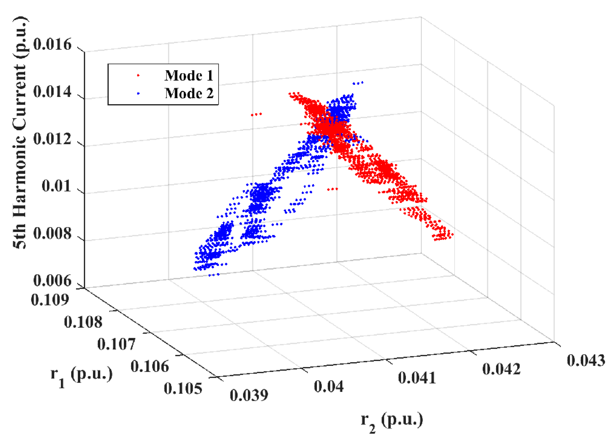
3.1. Case 1: 2880 Data Points, 2 Modes
In this subsection, we conduct a case study involving the parameter identification of two modes shown in Figure 3. The clustering results are shown in Figure 5. We can see that the data points with different colors belong to different modes, and two linear modes are separated clearly. The parameters of two linear modes are detailed in Table 2.
This case shows that the proposed DCMM is able to handle the linear clustering problem and obtain accurate parameters as Dc is calculated to be 3.27%.
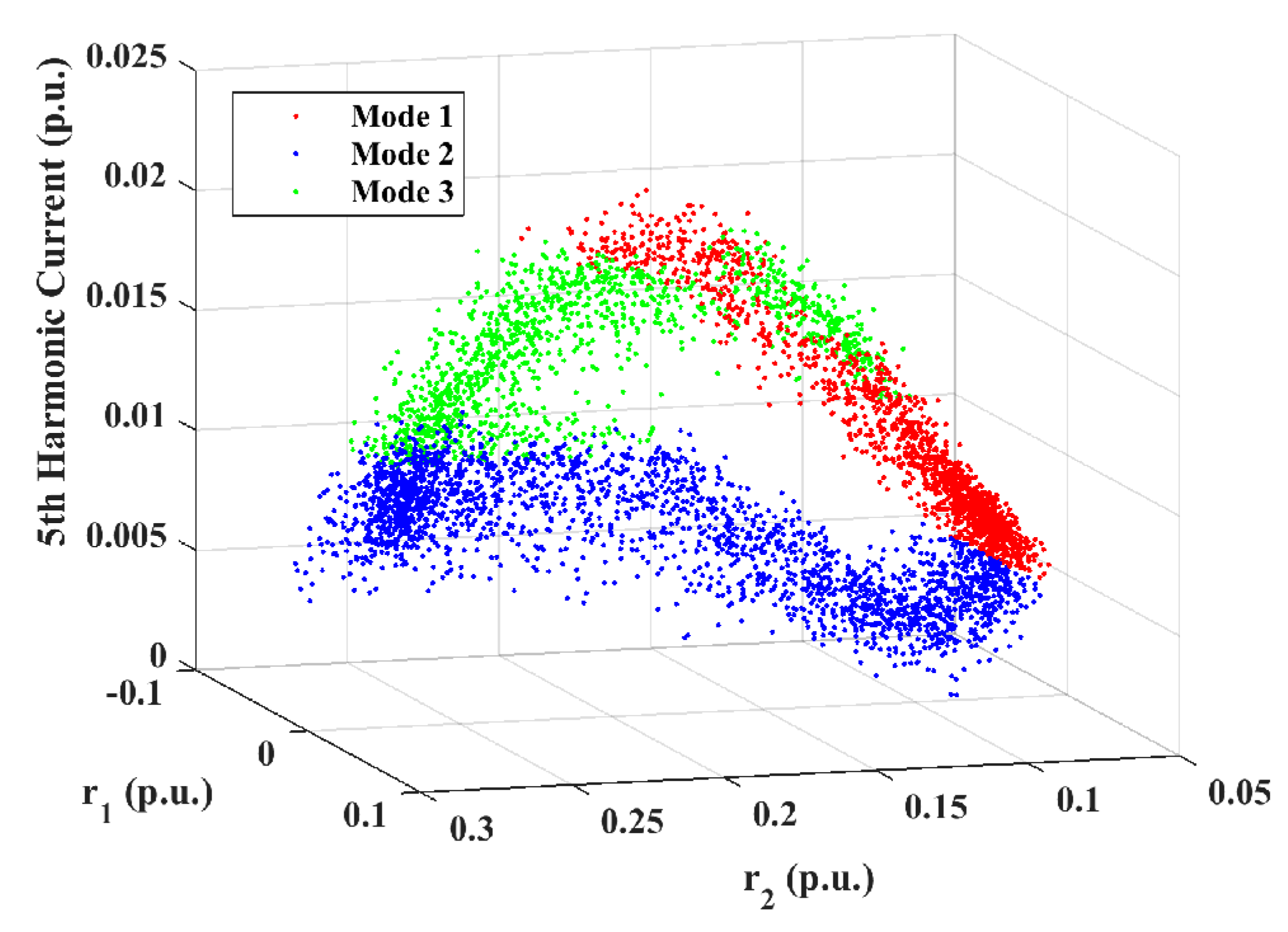
3.2. Case 2: 3360 Data Points, 3 Modes
The second case study involving the parameter identification of the three modes shown in Figure 4 was tested. The clustering results are shown in Figure 6. It can be seen that three linear modes are divided properly under the proposed DCMM. The parameters of the three linear modes are detailed in Table 3.
It can be found that the DCMM maintains its high precision when the test dataset changes observably because Dc is calculated to be 2.18% in this case.
3.3. Summary of Case 1 and 2
It can be observed that the DCMM is able to separate the intersecting linear modes exactly. The parameter identification results are accurate as the average estimation deviations of two cases are less than 5%. In other words, the proposed DCMM is effective in different scenes, even if the data volumes, number of clusters, and sample distributions change significantly.
4. Case Study
In this section, the DCMM was utilized to identify the parameters of the multi-mode EAF harmonic model based on the harmonic dataset. A comparison among the proposed model, the constant-harmonic-ratio-type model, and the Norton equivalent model was then implemented. Finally, the application of the multi-mode EAF harmonic model is introduced.
4.1. Parameter Identification of Multi-Mode EAF Harmonic Model
To obtain the harmonic data of the EAF, the EAF model simulating flicker disturbance was developed in Simulink. As shown in Figure 7, a three-phase EAF model connects a 0.4 kV, 1 MVA, 50 Hz three-phase source, where Z1 is the system impedance resulting from the minimum short-circuit capacity of the assumed source. The three-phase EAF model shown in Figure 7 is detailed in Figure 8; each EAF function block represents an electrode at each phase, and the controlled voltage source with a resistive and inductive network was adopted to model the flicker frequency and magnitude variation. The simulation time was set to 101 s, and the current and voltage signals extracted through a PQ recorder were analyzed every 0.02 s with a fixed sampling rate of 2500 Hz by the fast-Fourier transform (FFT) algorithm. Finally, we obtained 5000 sets of the fundamental current, the 2-nd to 25-th harmonic current, and the 2-nd to 25-th harmonic voltage peaks.
Taking the 5-th harmonic current as an example (the multi-mode EAF harmonic model of other frequencies can be also established by our method), the 5000 sets of the fundamental current, the 5-th harmonic current, and the 2-nd to 25-th harmonic voltage peaks are normalized according to the short-circuit capacity and base voltage, and the dimensions of the normalized dataset are reduced to 3-dimensions from 25-dimensions by PCA. In this case, 4000 sets of data shown in Figure 9 are employed to identify the parameters of the multi-mode EAF harmonic model and the remaining 1000 sets of data named the validation dataset are utilized to evaluate modeling accuracy.
The number of clusters of the modeling dataset was calculated to be 3. The clustering results are shown in Figure 10, the data points with different colors belong to different modes, it is can be found that three linear modes corresponding to three modes of the EAF smelting process are separated as desired. The simplified model parameters can be obtained and are listed in Table 4. In terms of Equation (8), the model parameters can be obtained.
4.2. Comparison of Different Models
The proposed DCMM was also adopted to establish the constant-harmonic-ratio-type model and the Norton equivalent model based on the modeling dataset, shown in Figure 9, respectively. To demonstrate the advantages of the proposed model, a comparison among the proposed model, the constant-harmonic-ratio-type model, and the Norton equivalent model was implemented based on the validation dataset. The evaluation indexes are shown as follows,
where ME represents the mean error, MSE is the mean square error, R2 denotes the coefficient of determination, FA is the fitting accuracy, N is the number of data points of validation dataset, It(i) and Ic(i), respectively, denote the true value and calculated value of the 5-th harmonic current of the i-th data point of the validation dataset, and I′ is the mean value of the 5-th harmonic current of the validation dataset.
The comparison results are demonstrated in Table 5 and it can be observed that both the ME and MSE of the proposed models are less than those of the other two models, therefore, the proposed model is more accurate than the other two models. Moreover, both the R2 and FA of the proposed model are greater than those of the other two models, thus, the fitting effect of the proposed model is optimal among the three models.
4.3. Application of Multi-Mode EAF Harmonic Model
In this subsection, the application of the multi-mode EAF harmonic model is elaborated. The process of the harmonic power-flow calculation based on the multi-mode EAF harmonic model is shown in Figure 11. The fundamental current is known since the fundamental power-flow calculation is carried out before the harmonic power-flow calculation. First, we set the initial values of harmonic voltages. Then, the values of harmonic currents are calculated based on Equation (4). Later, the harmonic currents are substituted into the harmonic power-flow equations to calculate new values of harmonic voltages. Finally, if the convergence condition is true, the new values of harmonic voltages are obtained, otherwise, return to Step 2.
Taking a mode of the 3-rd and 5-th multi-mode EAF harmonic models as an example, we calculated the 3-rd and 5-th harmonic voltages according to the process shown in Figure 11, respectively. The calculated results are demonstrated in Table 6, Zh denotes the h-th harmonic system impedance calculated based on the circuit diagram shown in Figure 7, Uh is the h-th harmonic voltage.
The probability distributions of the measured 3-rd and 5-th harmonic voltage data are shown in Figure 12. The blue lines denote the mean values of the measured 3-rd and 5-th harmonic voltages and the red lines denote the harmonic power-flow calculation results. It can be observed that the established multi-mode EAF harmonic models are effective in the harmonic power-flow calculation, as the deviations between the calculated values and the mean values of measured data are 3.10% and 2.40%, respectively.
5. Discussion
This paper proposes the DCMM for the multi-mode EAF harmonic model. When adopting the same algorithm (i.e., PSO-based K-means algorithm), the results show that the multi-mode EAF harmonic model is more accurate than the constant-harmonic-ratio-type model and the Norton equivalent model (see Table 5). The constant-harmonic-ratio-type model of EAF considers the interaction between the harmonic currents and the fundamental current but ignores the coupling relationship between the harmonic currents and harmonic voltages. The Norton equivalent model of EAF considers the impact of the harmonic voltages on the harmonic current in the same frequency but ignores the interaction among the harmonic currents, the fundamental current, and the harmonic voltages of different frequencies. As the correlation between the harmonic currents and fundamental current is more prominent than that between the harmonic currents and the harmonic voltage of the same frequency, therefore, the constant-harmonic-ratio-type model is more accurate than the Norton equivalent model. In our method, the proposed multi-mode EAF harmonic model considers the linear coupling relationship among the harmonic currents, the fundamental current, and the harmonic voltages, as shown in Equation (3). Therefore, the multi-mode EAF harmonic model is more accurate than the other two models. However, the increased model variables would inevitably lead to poor computational efficiency. To deal with such an issue, our method extracts the smaller representative dataset from a larger one to improve computational efficiency.
On the other hand, the DCMM based on the PSO-based K-means algorithm is elaborated in Section 2.2. Compared with the conventional K-means algorithm, it is more efficient for the PSO-based K-means algorithm to search for the near-global solution or global optimal solution, because high dimensional spatial data is preprocessed, and the optimal number of clusters and initial clustering centers are calculated. The performance evaluation results clearly show that the proposed DCMM is accurate in establishing the multi-mode model since the average estimation deviations are less than 5% under different experimental conditions. Moreover, the accuracy of the linear approximation of the proposed model introduced in Section 2.1 can be reflected by FA. As shown in Table 5, it can be found that the FA of the proposed model is at the desired level. However, the accuracy of the linear approximation of the proposed model may decrease when the small-scale modeling dataset is employed in EAF modeling as the outliers of the small-scale modeling dataset have a greater negative impact on the linear fitting than those of the large-scale modeling dataset.
6. Conclusions
This paper has developed the DCMM to establish the multi-mode EAF harmonic model to evaluate the harmonic pollution of EAF. The proposed DCMM fully considers the coupling relationship among different frequencies of harmonics while employing the PCA to improve computational efficiency. Furthermore, the proposed DCMM partitions the multi-mode EAF harmonic data into several clusters corresponding to the different modes of the EAF smelting process, and identifies the multi-mode EAF harmonic model parameters. Finally, the multi-mode EAF harmonic model was applied to the harmonic power-flow calculation to evaluate the harmonic pollution of EAF. The accuracy of the multi-mode EAF harmonic model was verified by carrying out the case study. Comparison results show that the multi-mode EAF harmonic model is more accurate than the other two models. In summary, the proposed DCMM is effective for evaluating the harmonic pollution of EAF, in this way, it improves the energy efficiency and productivity of EAF.
Note that the multi-mode harmonic model is suitable for EAF, which in practice, may not be applicable to other harmonic sources. Hence, our future research work will focus on studying the different multi-mode models for different harmonic sources.
Author Contributions
Conceptualization, Z.S.; methodology, Z.S.; software, H.X.; validation, H.X.; formal analysis, Z.S. and H.X.; investigation, H.X.; resources, F.C.; data curation, H.X.; writing—original draft preparation, H.X.; writing—review and editing, H.X., Z.S. and F.C.; visualization, H.X.; supervision, F.C.; project administration, Z.S.; funding acquisition, Z.S. and F.C.
Funding
This work was supported in part by the National Natural Science Foundation of China (Grant No. 51777035), in part by Fujian Province Natural Science Foundation of China (Grant No. 2017J01480), and in part by Scientific Research Staring Foundation of Fuzhou University (Grant No. 510773).
Conflicts of Interest
The authors declare no conflict of interest.
References
- Raul, G.S.; Javier, V.C.; Fernando, M.C.; Longoria-Gandara, O.; Ortegón Aguilar, J. Electric arc furnace modeling with artificial neural networks and arc length with variable voltage gradient. Energies 2017, 10, 1424. [Google Scholar]
- Gajic, D.; Savic-Gajic, I.; Savic, I.; Georgieva, O.; Di Gennaro, S. Modelling of electrical energy consumption in an electric arc furnace using artificial neural networks. Energy 2016, 108, 132–139. [Google Scholar] [CrossRef]
- Kirschen, M.; Badr, K.; Pfeifer, H. Influence of direct reduced iron on the energy balance of the electric arc furnace in steel industry. Energy 2011, 36, 6146–6155. [Google Scholar] [CrossRef]
- Steven, L.; Oyeniyi, O.; Christos, N.M.; Lazova, M.; Kaya, A.; Van den Broek, M.; De Paepe, M. Case study of an organic rankine cycle (ORC) for waste heat recovery from an electric arc furnace (EAF). Energies 2017, 10, 649–664. [Google Scholar]
- Oyeniyi, O.; Christos, M. Thermo-Economic and heat transfer optimization of working-fluid mixtures in a low-temperature organic rankine cycle system. Energies 2016, 9, 448–469. [Google Scholar]
- Horton, R.; Haskew, T.A.; Burch, R.F., IV. A time-domain ac electric arc furnace model for flicker planning studies. IEEE Trans. Power Deliv. 2017, 24, 1450–1457. [Google Scholar] [CrossRef]
- Cano-Plata, E.A.; Ustariz-Farfan, A.J.; Soto-Marin, O.J. Electric arc furnace model in distribution systems. IEEE Trans. Ind. Appl. 2015, 51, 4314–4320. [Google Scholar] [CrossRef]
- Hsu, Y.; Chen, K.; Huang, P.; Lu, C. Electric arc furnace voltage flicker analysis and prediction. IEEE Trans. Instrum. Meas. 2011, 60, 3360–3368. [Google Scholar] [CrossRef]
- Bhonsle, D.C.; Kelkar, R.B. Analyzing power quality issues in electric arc furnace by modeling. Energy 2016, 115, 830–839. [Google Scholar] [CrossRef]
- Chen, X.; Lin, J.; Wan, C.; Song, Y.; Luo, H. A unified frequency-domain model for automatic generation control assessment under wind power uncertainty. IEEE Trans. Smart Grid 2019, 10, 2936–2947. [Google Scholar] [CrossRef]
- Munoz, J.A.; Espinoza, J.R.; Baier, C.R.; Moran, L.A.; Espinosa, E.E.; Melin, P.E.; Sbarbaro, D.G. Design of a discrete-time linear control strategy for a multicell upqc. IEEE Trans. Ind. Electron. 2012, 59, 3797–3807. [Google Scholar] [CrossRef]
- Sezgin, E.; Göl, M.; Salor, Ö. State-Estimation-Based determination of harmonic current contributions of iron and steel plants supplied from PCC. IEEE Trans. Ind. Appl. 2016, 52, 2654–2663. [Google Scholar] [CrossRef]
- Göl, M.; Salor, O.; Alboyaci, B.; Mutluer, B.; Cadirci, I.; Ermis, M. A new field-data-based EAF model for power quality studies. IEEE Trans. Ind. Appl. 2010, 46, 1230–1242. [Google Scholar] [CrossRef]
- Vatankulu, Y.E.; Şentürk, Z.; Salor, O. Harmonics and interharmonics analysis of electrical arc furnaces based on spectral model optimization with high-resolution windowing. IEEE Trans. Ind. Appl. 2017, 53, 2587–2595. [Google Scholar] [CrossRef]
- Illahi, F.; El-Amin, I.; Mukhtiar, M.U. The application of multiobjective optimization technique to the estimation of electric arc furnace parameters. IEEE Trans. Power Deliv. 2018, 33, 1727–1734. [Google Scholar] [CrossRef]
- Mousavi Agah, S.M.; Hosseinian, S.H.; Abyaneh, H.A.; Moaddabi, N. Parameter identification of arc furnace based on stochastic nature of arc length using two-step optimization technique. IEEE Trans. Power Deliv. 2010, 25, 2859–2867. [Google Scholar] [CrossRef]
- Torabian Esfahani, M.; Vahidi, B. A new stochastic model of electric arc furnace based on hidden markov model: A study of its effects on the power system. IEEE Trans. Power Deliv. 2012, 27, 1893–1901. [Google Scholar] [CrossRef]
- Chen, C.; Chen, Y. A neural-network-based data-driven nonlinear model on time- and frequency-domain voltage–current characterization for power-quality study. IEEE Trans. Power Deliv. 2015, 30, 1577–1584. [Google Scholar] [CrossRef]
- Chang, G.W.; Chen, C.; Liu, Y. A neural-network-based method of modeling electric arc furnace load for power engineering study. IEEE Trans. Power Syst. 2010, 25, 138–146. [Google Scholar] [CrossRef]
- Chang, G.W.; Lin, S.; Chen, Y.; Lu, H.; Chang, Y. An advanced EAF model for voltage fluctuation propagation study. IEEE Trans. Power Deliv. 2017, 32, 980–988. [Google Scholar] [CrossRef]
- Naveros, F.; Luque, N.R.; Garrido, J.A.; Carrillo, R.R.; Anguita, M.; Ros, E. A spiking neural simulator integrating event-driven and time-driven computation schemes using parallel CPU-GPU co-processing: A case study. IEEE Trans. Neural Netw. Learn. Syst. 2015, 26, 1567–1574. [Google Scholar] [CrossRef] [PubMed]
- Matsubara, T.; Torikai, H. An asynchronous recurrent network of cellular automaton-based neurons and its reproduction of spiking neural network activities. IEEE Trans. Neural Netw. Learn. Syst. 2016, 27, 836–852. [Google Scholar] [CrossRef]
- Gao, S.; Li, X.; Ma, X.; Hu, H.; He, Z.; Yang, J. Measurement-Based compartmental modeling of harmonic sources in traction power-supply system. IEEE Trans. Power Deliv. 2017, 32, 900–909. [Google Scholar] [CrossRef]
- Ranade, S. Task force on harmonic modeling and simulation. Modeling and simulation of the propagation of harmonics in electric power networks. I. Concepts, models, and simulation techniques. IEEE Trans. Power Deliv. 1996, 11, 452–465. [Google Scholar]
- Ajaei, F.B.; Afsharnia, S.; Kahrobaeian, A.; Farhangi, S. A Fast and effective control scheme for the dynamic voltage restorer. IEEE Trans. Power Deliv. 2011, 26, 2398–2406. [Google Scholar] [CrossRef]
- Salles, D.; Jiang, C.; Xu, W.; Freitas, W.; Mazin, H.E. Assessing the collective harmonic impact of modern residential loads—Part I: Methodology. IEEE Trans. Power Deliv. 2012, 27, 1937–1946. [Google Scholar] [CrossRef]
- Papaioannou, I.T.; Alexiadis, M.C.; Demoulias, C.S.; Labridis, D.P.; Dokopoulos, P.S. Modeling and field measurements of photovoltaic units connected to LV grid. Study of penetration scenarios. IEEE Trans. Power Deliv. 2011, 26, 979–987. [Google Scholar] [CrossRef]
- Yang, P.; Tsai, J.; Chou, J. PCA-Based fast search method using PCA-LBG-based VQ codebook for codebook search. IEEE Access 2016, 4, 1332–1344. [Google Scholar] [CrossRef]
- Taşkın, G.; Kaya, H.; Bruzzone, L. Feature selection based on high dimensional model representation for hyperspectral images. IEEE Trans. Image Process. 2017, 26, 2918–2928. [Google Scholar] [CrossRef]
- Jia, S.; Tang, G.; Zhu, J.; Li, Q. A novel ranking-based clustering approach for hyperspectral band selection. IEEE Trans. Geosci. Remote Sens. 2016, 54, 88–102. [Google Scholar] [CrossRef]
- Fan, Y.; Gongshen, L.; Kui, M.; Zhaoying, S. Neural feedback text clustering with BiLSTM-CNN-kmeans. IEEE Access 2018, 6, 57460–57469. [Google Scholar] [CrossRef]
- Huang, X.; Ye, Y.; Zhang, H. Extensions of kmeans-type algorithms: A new clustering framework by integrating intracluster compactness and intercluster separation. IEEE Trans. Neural Netw. Learn. Syst. 2014, 25, 1433–1446. [Google Scholar] [CrossRef] [PubMed]
- Peng, K.; Leung, V.C.M.; Huang, Q. Clustering approach based on mini batch kmeans for intrusion detection system over big data. IEEE Access 2018, 6, 11897–11906. [Google Scholar] [CrossRef]
- Zhang, Y.; Chiang, H. A novel consensus-based particle swarm optimization-assisted trust-tech methodology for large-scale global optimization. IEEE Trans. Cybern. 2017, 47, 2717–2729. [Google Scholar] [CrossRef]
- Zhang, Y.; Chen, X.Q.; Zhan, T.M.; Jiao, Z.Q.; Sun, Y.; Chen, Z.-M.; Yao, Y.; Fang, L.T.; Lv, Y.-D.; Wang, S.-H. Fractal dimension estimation for developing pathological brain detection system based on minkowski-bouligand method. IEEE Access 2016, 4, 5937–5947. [Google Scholar] [CrossRef]
Figure 1.
The process of the proposed data-driven compartmental modeling method (DCMM).

Figure 2.
The clustering process.

Figure 3.
Dataset of case 1.

Figure 4.
Dataset of case 2.

Figure 5.
Clustering results of case 1.

Figure 6.
Clustering results of case 2.

Figure 7.
Simplified circuit diagram for data measurement of the electric arc furnace (EAF).

Figure 8.
EAF model simulating flicker disturbance.

Figure 9.
Modeling dataset.

Figure 10.
Clustering results of the 5-th harmonic dataset of the EAF.

Figure 11.
The process of harmonic power-flow calculation.

Figure 12.
The probability distributions of the measured data.


Table 1.
The true values of the simplified model parameters of case 1 and 2.
| Case | Mode | Ap | C |
|---|---|---|---|
| Case 1 | Mode 1 | [3.7099, −1.1922] | −0.0115 |
| Mode 2 | [−3.9041, −0.3421] | −0.2107 | |
| Case 2 | Mode 1 | [3.7099, −1.1922] | −0.0115 |
| Mode 2 | [−3.9041, −0.3421] | −0.2107 | |
| Mode 3 | [0.3511, −0.8861] | −0.0904 |
Table 2.
The estimated values of the simplified model parameters of case 1.
| Case | Mode | Ap′ | C′ |
|---|---|---|---|
| Case 1 | Mode 1 | [3.7338, −1.2106] | −0.0110 |
| Mode 2 | [−3.8913, −0.3801] | −0.2142 |
Table 3.
The estimated values of the simplified model parameters of case 2.
| Case | Mode | Ap′ | C′ |
|---|---|---|---|
| Case 2 | Mode 1 | [3.7305, −1.2161] | −0.0098 |
| Mode 2 | [−3.8886, −0.790] | −0.2140 | |
| Mode 3 | [0.3510, −0.8861] | −0.0904 |
Table 4.
The simplified model parameters of the 5-th harmonic of the EAF.
| Case | Mode | Ap | C |
|---|---|---|---|
| EAF | Mode 1 | [0.1111, −0.0095] | −0.0007 |
| Mode 2 | [0.0283, 0.0099] | 0.0020 | |
| Mode 3 | [−0.0164, 0.1193] | 0.0203 |
Table 5.
Comparison results of the different models.
| Model | ME | MSE | R2 | FA |
|---|---|---|---|---|
| Proposed model | 1.1369 | 2.0536 | 90.28% | 98.25% |
| Constant-harmonic-ratio-type model | 1.2862 | 2.5837 | 87.78% | 96.80% |
| Norton equivalent model | 1.6345 | 4.2531 | 79.88% | 95.38% |
Table 6.
The harmonic power-flow calculation results.
| Order | Zh (ohms) | Uh (V) |
|---|---|---|
| 3 | 0.039 + 0.882i | 30.4131 |
| 5 | 0.039 + 1.372i | 18.2623 |
© 2019 by the authors. Licensee MDPI, Basel, Switzerland. This article is an open access article distributed under the terms and conditions of the Creative Commons Attribution (CC BY) license (http://creativecommons.org/licenses/by/4.0/).
Share and Cite
MDPI and ACS Style
Xu, H.; Shao, Z.; Chen, F. Data-Driven Compartmental Modeling Method for Harmonic Analysis—A Study of the Electric Arc Furnace. Energies 2019, 12, 4378. https://doi.org/10.3390/en12224378
AMA Style
Xu H, Shao Z, Chen F. Data-Driven Compartmental Modeling Method for Harmonic Analysis—A Study of the Electric Arc Furnace. Energies. 2019; 12(22):4378. https://doi.org/10.3390/en12224378
Chicago/Turabian StyleXu, Haobo, Zhenguo Shao, and Feixiong Chen. 2019. "Data-Driven Compartmental Modeling Method for Harmonic Analysis—A Study of the Electric Arc Furnace" Energies 12, no. 22: 4378. https://doi.org/10.3390/en12224378
Note that from the first issue of 2016, this journal uses article numbers instead of page numbers. See further details here.