A Comprehensive Methodology for the Integrated Optimal Sizing and Operation of Cogeneration Systems with Thermal Energy Storage

Abstract

Cogeneration systems are widely acknowledged as a viable solution to reduce energy consumption and costs, and CO₂ emissions. Nonetheless, their performance is highly dependent on their capacity and operational strategy, and optimization methods are required to fully exploit their potential. Among the available technical possibilities to maximize their performance, the integration of thermal energy storage is recognized as one of the most effective solutions. The introduction of a storage device further complicates the identification of the optimal equipment capacity and operation. This work presents a cutting-edge methodology for the optimal design and operation of cogeneration systems with thermal energy storage. A two-level algorithm is proposed to reap the benefits of the mixed integer linear programming formulation for the optimal operation problem, while overcoming its main drawbacks by means of a genetic algorithm at the design level. Part-load effects on nominal efficiency, variation of the unitary cost of the components in relation to their size, and the effect of the storage volume on its thermal losses are considered. Moreover, a novel formulation of the optimization problem is proposed to better characterize the heat losses and operation of the thermal energy storage. A rolling-horizon technique is implemented to reduce the computational time required for the optimization, without affecting the quality of the results. Furthermore, the proposed methodology is adopted to design a cogeneration system for a secondary school in San Francisco, California, which is optimized in terms of the equivalent annual cost. The results show that the optimally sized cogeneration unit directly meets around 70% of both the electric and thermal demands, while the thermal energy storage additionally covers 16% of the heat demands.

1. Introduction

Cogeneration or combined heat and power (CHP) systems are defined as energy generation units that simultaneously produce electric (or mechanical) energy and useful heat from a single fuel source [1]. The role of cogeneration in the process of reducing primary energy consumption, CO₂ emissions, and energy costs is widely acknowledged [2]. This is mainly due to the higher energy efficiency achievable by CHP systems compared to the separate generation of electricity and heat. Moreover, cogeneration systems are considered a viable solution to promote the development of microgrids with distributed renewable energy [3].

Nevertheless, the energy, environmental, and economic performances of CHP systems are highly dependent on their sizing and operational strategy. Indeed, undersizing and oversizing of cogeneration plants are frequent and may compromise the energy saving potential of those systems [4]. For this reason, several methods have been proposed in recent years to identify the integrated optimal sizing and management of CHP plants. A non-exhaustive list of selected examples is as follows. Gimelli et al. [5] presented a multi-objective optimization approach, based on a genetic algorithm, for the optimal design of modular cogeneration systems based on reciprocating gas engines. A sensitivity analysis was performed to evaluate the robustness of the optimal solution with respect to energetic, legislative, and market scenarios. Similarly, Beihong and Weiding [6] proposed a mixed integer non-linear programming (MINLP) formulation to determine the capacity of a gas turbine cogeneration plant that minimizes the annual total cost, thus proving the importance of optimization methods in the design and operation of CHP systems. On the same topic, Aviso and Tan [7] applied a different optimization tool, namely the fuzzy P-graph approach, for the optimal design of cogeneration and trigeneration systems. This approach allows the consideration of soft constraints on user demand and fuel availability. Likewise, Urbanucci and Testi [8] proposed a probabilistic methodology for the optimal sizing of CHP units under uncertainty in energy demands, based on a Monte Carlo risk analysis. Moreover, the thermoeconomic approach was also applied to cogeneration systems, as in [9], where Yokoyama et al. optimized both the exergy efficiency and the annual cost of a CHP gas turbine.

Even though the above-mentioned works are significant examples of optimization methodologies for cogeneration units, none of them consider a storage device in the energy system. Nevertheless, integrating thermal energy storages (TESs) into CHP systems can lead to higher operational flexibility and better overall performance. Indeed, as shown in [10] by Fang and Lahdelma, the decoupling of heat and electric demands by storing the exceeding CHP thermal production allows maximization of the operation of cogeneration systems, thus reducing the load share covered by back-up units. During the years, several approaches for the optimization of cogeneration systems with storage devices have been proposed. For example, Kuang et al. [11] applied a dynamic programming technique to define the most economical operation schedule of trigeneration systems. Elsido et al. [12] proposed a MINLP formulation for a district heating network, combining evolutionary algorithms with mathematical programming. The optimal design and operation for both economic and environmental objectives of a CHP system with a thermal storage tank was investigated by Fuentes-Cortés et al. [13], by exploiting commercial MINLP solvers.

The introduction of energy storage units makes the optimization of CHP systems significantly more complicated. In the absence of TES, the operation optimization problem can be considered “static”, since each timestep is independent of the others. Under this condition, it can be proven that the overall optimum corresponds to the sum of the optimums of every single timestep [14]. Consequently, the optimal solution can be traced back to the solution of several optimization problems, one for each timestep, which, compared to the overall problem, are characterized by a lower dimensionality and, hence, by a lower computational cost. On the other hand, when a storage device is considered within the system, the problem becomes “dynamic”, because of the dependency between the optimization variables of adjacent timesteps. This results in a higher dimensionality—thus, a higher computational cost—of the optimization problem, which calls for the adoption of decomposition strategies, like the so-called rolling-horizon approach. Rolling-horizon techniques have been proven to effectively tackle the high dimensionality of optimization problems, by decomposing the problem in shorter periods, without affecting the quality of the results [15].

The general problem of the integrated optimal sizing and operation of cogeneration systems usually results in a non-linear problem. Among the available optimization techniques, the state-of-the-art approach to solve this problem consists in linearizing the original problem to obtain a mixed integer linear programming (MILP) problem [12]. This is mainly due to the guarantee of the global optimality of the solution and to the effectiveness of the available commercial MILP solvers. Nonetheless, when dealing with the optimal design problem, with the size of each component an optimization variable, strong assumptions have to be made to retain the linearity of the model: The efficiency of the units must be kept constant, the variation of the unitary cost of the components in relation to their size must be neglected, and the temperature of the storage cannot be directly tracked [14]. To tackle those issues, a decomposition approach based on a two-level optimization algorithm is adopted in this work. At the upper level, the optimal design problem (i.e., the selection of CHP and storage capacities) is solved by means of a metaheuristic method, while at the lower level, the operational strategy is optimized by means of an MILP method. The design and operation problems must be solved simultaneously since they are intrinsically linked.

As already mentioned, the decomposition approach allows tracking of the average temperature of the storage in each timestep, and a better estimate of the thermal losses can be performed by considering also the impact of the storage geometrical characteristics. Indeed, in simpler models, the storage is seen as a simplified thermal battery, and its losses are assumed proportional to the energy content of the storage with a constant heat-loss coefficient, thus providing a poor physical representation of the system, as shown in [15,16]. In this paper, on the basis of the model proposed by Steen et al. [16], a new formulation of the optimization problem is developed, capable of considering the impact of geometrical characteristics, the tank’s insulation properties, and the ambient conditions in the evaluation of TES heat losses. As well as including all the above-mentioned features, the main innovation of the proposed approach is the possibility of simulating and optimizing the operation of the storage when the temperature of the TES is below the operation threshold temperature. Furthermore, since the thermal storage makes the operation optimization problem “dynamic” and, consequently, computationally very expensive, a rolling-horizon approach is proposed.

To summarize, the main purpose and novelty of this study is to develop a comprehensive methodology for the integrated optimal sizing and operation of cogeneration systems with thermal energy storage. To the best of the authors’ knowledge, such a comprehensive approach is still missing. In view of this, the present paper aims to propose a thorough methodology with the following key characteristics:

• A decomposition approach was adopted. At the upper level, the optimal design problem is solved by means of a genetic algorithm, while at the lower level, a MILP formulation is adopted to identify the optimal operation;
• A novel MILP formulation for the TES was developed to obtain a better assessment of its optimal operation;
• A rolling-horizon technique was implemented to reduce the computational time of the optimization problem.

Finally, the proposed methodology was tested in a case study. To this end, hourly electric and thermal demands of a reference building (a secondary school located in San Francisco, California) were considered, and the optimal integrated sizing and operation of a cogeneration system with thermal energy storage were identified.

The rest of the paper is structured as follows. In Section 2, the methodological framework is described: The energy system, the TES modeling, the optimization problem, and algorithm are presented in detail. Section 3 presents the case study, while an in depth-analysis of the results follows in Section 4. The last section contains concluding remarks.

2. Methodology

2.1. The Energy System

The energy system under consideration is schematically shown in Figure 1. It comprises a cogeneration unit (e.g., an internal combustion engine), a thermal energy storage, and an auxiliary boiler. Moreover, the exchange of electricity with the regional grid is allowed (both selling and buying). Thus, the thermal demand can be met partly by the CHP heat production and partly by the boiler, while the electric demand can be covered partly by the CHP electric production and partly by the electric grid. The TES can be used to store the thermal energy recovered from the cogeneration unit and, subsequently, to cover the thermal demand.

An hourly timestep was adopted for the simulation of the system, as a compromise between the computational burden and temporal resolution of the scheduling problem. With this timestep length, the behavior of the machines based on the hourly energy flows can be considered, thus averaging the transient performances, which occur on shorter time scales. Indeed, among the considered generators, the internal combustion engine is the one with the longest dynamic response, with start-up times of around 2 minutes for the electric output and less than 15 minutes for the thermal output [17].

2.2. Thermal Energy Storage Modeling

A cylindrical water tank is considered as the sensible-heat TES device. At each i-th timestep, an equivalent TES temperature ($T_{TES}$) is defined on the basis of the stored energy ($H_{tot,TES}^i$), so that the following relationship holds:

$$H_{tot,TES}^i={\rho }_{TES}{V}_{TES}{c}_{TES}\left(T_{TES}^i-T_{amb}^i\right)$$

(1)

with ${\rho }_{TES}$ as the water density, $V_{TES}$, the storage volume, $c_{TES}$, the specific heat of water, and $T_{TES}$, the ambient temperature. In this way, the zero state of charge is the one corresponding to an equivalent TES temperature equal to the ambient temperature. The dynamic of the stored energy varies according to the following energy balance:

$$H_{tot,TES}^{i+1}-H_{tot,TES}^i=-H_{TES,loss}^i+H_{TES,charge}^i-H_{TES,discharge}^i$$

(2)

with $H_{TES,losses}^i$ as the storage losses, whose formulation is discussed in detail below, and $H_{TES,charge}^i$ and $H_{TES,discharge}^i$ as the energy delivered to and from the storage, respectively.

With the useful energy only a fraction of the whole TES energy content, due to the minimum temperature level that is useful to satisfy the thermal demand ($T_{u,TES}$), the energy stored is considered as the sum of two terms: The useful available energy ($H_{u,TES}^i$) and the residual energy ($H_{res,TES}^i$):

$$H_{tot,TES}^i=H_{u,TES}^i+H_{res,TES}^i$$

(3)

where:

$$H_{u,TES}^i={\rho }_{TES}{V}_{TES}{c}_{TES}\left(T_{TES}^i-T_{u,TES}\right)$$

(4)

$$H_{res,TES}^i={\rho }_{TES}{V}_{TES}{c}_{TES}\left(T_{u,TES}-T_{amb}^i\right)$$

(5)

This distinction is also useful to highlight differences between the models available in the current literature to evaluate thermal-storage losses. In simpler models, the storage is seen as a simplified thermal battery, and its losses are accounted for only on the basis of the useful storage energy content by means of a constant heat-loss coefficient [16]:

$$H_{TES,loss}^i={\theta }_{TES,loss}{H}_{u,TES}^i$$

(6)

with:

$${\theta }_{TES,loss}=\raisebox{1ex}{$U_{TES}{A}_{TES}\tau $}\!\left/ \!\raisebox{-1ex}{${\rho }_{TES}{V}_{TES}{c}_{TES}$}\right.$$

(7)

Nevertheless, Equation (6), by considering only the contribution of the useful energy (“dynamic” losses) and neglecting that related to the residual energy (“static” losses), leads to an underestimation of the losses. Indeed, it has been shown by Omu et al. [18] that considering static heat losses improves the accuracy of thermal-storage modeling, compared to a simplified thermal-battery model. To this end, different formulations that also consider the residual energy in the computation of the losses have been proposed [13]. The latter reads:

$$H_{TES,losses}^i=H_{dynamic,losses}^i+H_{static,losses}^i={\theta }_{TES,loss}{H}_{u,TES}^i+{\theta }_{TES,loss}{H}_{res,TES}^i$$

(8)

The use of these models leads to an additional issue when the coupled problem of sizing and operation is considered in the MILP formulation. Indeed, as it can be seen from Equations (6) and (7), the heat losses depend on the amount of stored energy, as well as on the capacity and characteristics of the TES, such as the volume of the tank and the overall heat transfer coefficient. Consequently, by considering a constant overall heat-loss coefficient, the impact of these optimization parameters—specifically of the volume of the tank—on the storage losses is neglected, thus affecting the solution of the optimization problem. To overcome this issue, in the present work, the decomposition of the optimization problem at the design level and operation level was adopted, as described in the next section. By doing so, the effect of the volume of the tank on the heat-loss coefficient can be exactly considered. Thus, a model capable of considering both the energy and the sizing parameters in the storage heat-losses formulation is developed as follows.

From Equation (7), it can be seen that once the overall heat-transfer coefficient is identified, the value of the heat-loss coefficient can be expressed as a function of the surface of the storage tank, which in turn is a function of the storage volume. To this end, once the aspect ratio (λ) of the tank is defined, the relation between the surface and the volume of the storage tank can be formulated as follows:

$$\lambda =h_{TES}/{\varphi }_{TES}$$

(9)

$$\raisebox{1ex}{$A_{TES}$}\!\left/ \!\raisebox{-1ex}{$V_{TES}$}\right.=\raisebox{1ex}{$\left(\pi {\varphi }_{TES}{h}_{TES}+\frac{\pi }{2}{\varphi }_{TES}^2\right)$}\!\left/ \!\raisebox{-1ex}{$\pi \frac{{\varphi }_{TES}^2}{4}{h}_{TES}$}\right.=\left(\raisebox{1ex}{$\left(4 \lambda +2\right)$}\!\left/ \!\raisebox{-1ex}{$2 \lambda $}\right.\right){\left(\raisebox{1ex}{$2 \pi \lambda $}\!\left/ \!\raisebox{-1ex}{$V_{TES}$}\right.\right)}^{1/3}$$

(10)

and the heat-loss coefficient can be finally expressed as a function of the volume of the storage tank:

$${\theta }_{TES,loss}=\left(\raisebox{1ex}{$U_{TES}\tau $}\!\left/ \!\raisebox{-1ex}{${\rho }_{TES}{c}_{TES}$}\right.\right)\left(\raisebox{1ex}{$\left(4 \lambda +2\right)$}\!\left/ \!\raisebox{-1ex}{$2 \lambda $}\right.\right){\left(\raisebox{1ex}{$2 \pi \lambda $}\!\left/ \!\raisebox{-1ex}{$V_{TES}$}\right.\right)}^{1/3}$$

(11)

In this way, the approach of the fixed thermal efficiency of the storage, commonly found in the literature, can be overcome, and the thermal losses of the TES can be expressed as a function of the thermophysical and geometrical properties of the storage tank and medium, and the temperatures of the ambient surroundings and the storage itself.

Finally, the energy balance of the TES reads:

$$\begin{array}{cc}\hfill H_{u,TES}^{i+1}+H_{res,TES}^{i+1}& \\ & =H_{res,TES}^i+\left(1-{\theta }_{TES,loss}\right)H_{u,TES}^i-{\theta }_{TES,loss}{H}_{res,TES}^i+H_{TES,charge}^i\hfill \\ & -H_{TES,discharge}^i\hfill \end{array}$$

(12)

and the following linear constraints must be considered:

$$H_{u,TES}^i\ge -H_{res,TES}^i$$

(13)

$$H_{tot,TES}^i\le H_{tot,TES,max}^i$$

(14)

$$0\le H_{TES,charge}^i\le Q_{TES,charge,max}·\tau$$

(15)

$$0\le H_{TES,discharge}^i\le Q_{TES,discharge,max}·\tau ·{\delta }_{TES}^i$$

(16)

$${\delta }_{TES}^i\le \left[\raisebox{1ex}{$H_{u,TES}^{i+1}$}\!\left/ \!\raisebox{-1ex}{${\rho }_{TES}{V}_{TES}{c}_{TES}\left(T_{u,TES}-T_{amb}^i\right)$}\right.\right]+1$$

(17)

In Equations (16) and (17), ${\delta }_{TES}^i$ is a binary variable, equal to 1 if the storage temperature in the i-th timestep is above its operational threshold, and, therefore, energy can be taken from the storage; otherwise, if the temperature of the storage is lower than $T_{u,TES}$, ${\delta }_{TES}^i$ is equal to 0 and no useful energy can be taken from the TES. The introduction of this binary variable allows a more accurate simulation and optimization of the operation of the storage. Indeed, in traditional MILP formulations, the temperature of the storage cannot drop below its operation threshold, which is unrealistic and limits the operation optimization.

Moreover, Equations (15) and (16) define the maximum amounts of energy that can be charged and discharged in a single timestep, respectively. If external plate heat exchangers are considered for both the charging and discharging the storage, those quantities coincide with the capacity of the heat exchangers themselves. Therefore, $Q_{TES,charge,max}$ and $Q_{TES,discharge,max}$ can be considered as design variables and are subject to optimization, once the investment cost of the plate heat exchangers is considered separately from that of the water storage tank.

2.3. Optimization Problem and Algorithm

The objective function to be minimized is the equivalent annual cost ($K$) of the system, which is calculated over the period of one year and composed of the annualized investment cost for the technologies, $I$, and the total annual operating cost, $O$:

$$K=I+O$$

(18)

$$I={{\displaystyle \sum }}_{j=1}^3{\alpha }_j·{\xi }_j^{{\beta }_j}·{\mathsf{\Gamma }}_j$$

(19)

where ${\xi }_j$ is the capacity of the j-th component to be installed (expressed in kW for the CHP, the boiler, and the plate heat exchangers, and in m³ for the TES), ${\alpha }_j$ and ${\beta }_j$ are the correlation parameters of the equipment cost as a function of the capacity, and $\mathsf{\Gamma }$ is the capital-recovery factor [19]:

$${\mathsf{\Gamma }}_j=\frac{r{\left(r+1\right)}^{l_j}}{{\left(r+1\right)}^{l_j}-1}$$

(20)

The total annual operating cost comprises the cost for purchasing electricity and natural gas and the revenue from selling electricity to the grid:

$$O={{\displaystyle \sum }}_{i=1}^{8760}\left[C_F\left(F_{CHP}^i+F_B^i\right)+C_{PE}{E}_P^i-C_{SE}{E}_S^i\right]$$

(21)

The optimization variables can be distinguished into two main groups: Sizing variables ($P_{CHP,nom}$, $V_{TES}$, $Q_{B,nom}$, $Q_{TES,charge,max}$, $Q_{TES,dischharge,max}$) and operation variables ($E_{CHP}^i$, $E_S^i$, $E_P^i$, $H_B^i$, $H_{TES,charge}^i$, $H_{TES,discharge}^i$).

Demand constraints must be satisfied in each i-th timestep:

$$H_{CHP}^i+H_B^i+H_{TES,discharge}^i·{\eta }_{TES,discharge}-H_{TES,charge}^i/{\eta }_{TES,charge}\ge H_d^i$$

(22)

$$E_{CHP}^i+E_P^i-E_S^i=E_d^i$$

(23)

In addition to the energy balance and constraints for the TES (Equations (12)–(17)) shown in Section 2.1), the following constraints and equations must be considered too:

$$E_{CHP}^i\le P_{CHP,nom}{\delta }_{CHP}^i$$

(24)

$$E_{CHP}^i\ge P_{CHP,min}{\delta }_{CHP}^i$$

(25)

$$H_{CHP}^i=P_{CHP}^i\frac{{\eta }_{H,CHP}}{{\eta }_{E.CHP}}$$

(26)

$$F_{CHP}^i=P_{CHP}/{\eta }_{E,CHP}$$

(27)

$$H_B^i\le Q_{B,nom}$$

(28)

$$F_B^i=H_B^i/{\eta }_B$$

(29)

$${\eta }_{E,CHP}={\eta }_{E,CHP,nom}\left(a_{E,CHP}{L}_{CHP}+b_{E,CHP}\right)$$

(30)

$${\eta }_{H,CHP}={\eta }_{H,CHP,nom}\left(a_{H,CHP}{L}_{CHP}+b_{H,CHP}\right)$$

(31)

where $L_{CHP}$ is the load factor of the cogeneration unit, defined as $L_{CHP}=F_{CHP}·{\eta }_{E,CHP,nom}/P_{CHP,nom}$, and ${\delta }_{CHP}^i$ is a binary variable equal to 1 when the CHP is on and equal to 0 when it is off. Equations (30) and (31) linearize the relationship between the electric and thermal efficiencies of the cogeneration unit with respect to its load factor, respectively.

Finally, the overall problem consists in the minimization of the equivalent annual cost:

$$minimize \left\{K\right\}$$

(32)

which results in a mixed integer non-linear optimization problem, because of the non-linear variations of the unitary cost of the components in relation to their capacity, the part-load effects on CHP efficiencies, and the thermal energy storage model (the dependency of ${\theta }_{TES,tot,loss}$ and ${\delta }_{TES}^i$ on $V_{TES}$).

To this aim, the overall problem was decomposed into two levels and the optimization variables distinguished into two categories, as schematically summarized in Figure 2. At the upper level, the synthesis/design problem, which identifies the components that should be included in the energy system and their capacities, is addressed by a genetic algorithm (GA). At the lower level, the optimal operation problem is solved by means of an MILP technique. The two problems are nested in each other and therefore they must be solved simultaneously. For each individual solution (components size) produced by the GA, the optimal annual operation cost is identified by the MILP solver, and, thus, the total EAC is calculated. This procedure is repeated for each individual of each generation produced by the GA, until the stopping criteria is met.

As already mentioned, this decomposition allows the benefits of the MILP formulation to be reaped, while overcoming its main drawbacks. Indeed, the part-load behavior of the CHP unit is considered, the variation of the unitary cost of the components in relation to their size is not neglected, and the effect of the storage volume on its heat-loss coefficient is taken into account.

The optimization was performed by using scripts written in the MATLAB environment. The commercial solver, CPLEX [20], for the MILP optimization and the MATLAB Genetic Algorithm Solver [21] were used. The settings and parameters adopted for the optimization algorithms are shown in

Table 1. Settings and parameters for the optimization algorithms.

MILP		Genetic Algorithm
MaxIter:	9.2234e+18	PopulationSize:		‘50’
Algorithm:	‘auto’	EliteCount:		‘0.05*PopulationSize’
BranchStrategy:	‘maxinfeas’	CrossoverFraction:		0.8000
MaxNodes:	9.2234e+18	MigrationDirection:		‘forward’
MaxTime:	1.0000e+75	MigrationInterval:		20
NodeDisplayInterval:	20	MigrationFraction:		0.2000
NodeSearchStrategy:	‘bn’	Generations:		‘400’
TolFun:	1.0000e-06	StallGenLimit:	50	StallTest:	‘averageChange’
TolRLPFun:	1.0000e-06	TolFun:		1.0000e-06
TolXInteger:	1.0000e-05	TolCon:		1.0000e-03

.

2.4. Rolling-Horizon Approach for the Decomposition of the Operation Problem

As stated above, the introduction of the storage in the energy system makes the operation optimization problem “dynamic”, because of the dependency between the optimization variables of adjacent timesteps. Therefore, once the sizes of the components are fixed, the problem of the minimization of the operational costs should be solved simultaneously for the whole optimization period (e.g., one year with an hourly resolution). This results in a very large number of variables and constraints, thus making the problem very challenging from the computational point of view [14]. To tackle this issue, the rolling-horizon procedure can be adopted, which consists in dividing the investigated period into smaller periods and optimizing each subproblem in sequence [22,23].

The rolling-horizon approach is schematically represented in Figure 3. The length of each sub-period of optimization is called “prediction horizon”. Once the solution for a certain sub-period is found, it can be implemented for one or a few timesteps (the total duration of which is called the “control horizon”). Then, the problem is solved for the following sub-period, and so on, until the problem is solved for the whole optimization period.

Therefore, the original operation problem is divided in $N=8760/k$ subproblems, which optimize the operation in $p$ consecutive timesteps:

$$min\left\{{{\displaystyle \sum }}_{i=n·c+1}^{i=n·c+p}\left[C_F\left(F_{CHP}^i+F_B^i\right)+C_{PE}{E}_P^i-C_{SE}{E}_S^i\right]\right\}$$

(33)

where $n$ goes from $0$ to $\left(N-1\right)$, $k$ is the length of the control horizon, and $p$ is the length of the prediction horizon (both measured in the number of timesteps). All the other constraints and relationships considered for the whole operation optimization problem must still be considered and remain the same.

Two parameters must be set in the rolling-horizon decomposition of the operation problem: The length of the prediction and control horizons. As the former increases and the latter decreases, the overall solution becomes more and more accurate, until it coincides with the exact solution (i.e., the solution of the whole optimization period considered at once). On the other hand, as the prediction horizon becomes shorter and the control horizon gets longer, the computational time decreases. Therefore, a compromise must be achieved between these two conflicting objectives.

Moreover, as the size of the thermal energy storage increases, the minimum length of the rolling-horizon so that the solution is not different from the whole-period-at-once solution increases too [24]. On the contrary, when no storage is included in the system, the problem becomes “static” and each timestep can be solved separately [25].

3. Case Study Presentation

3.1. Energy Demand

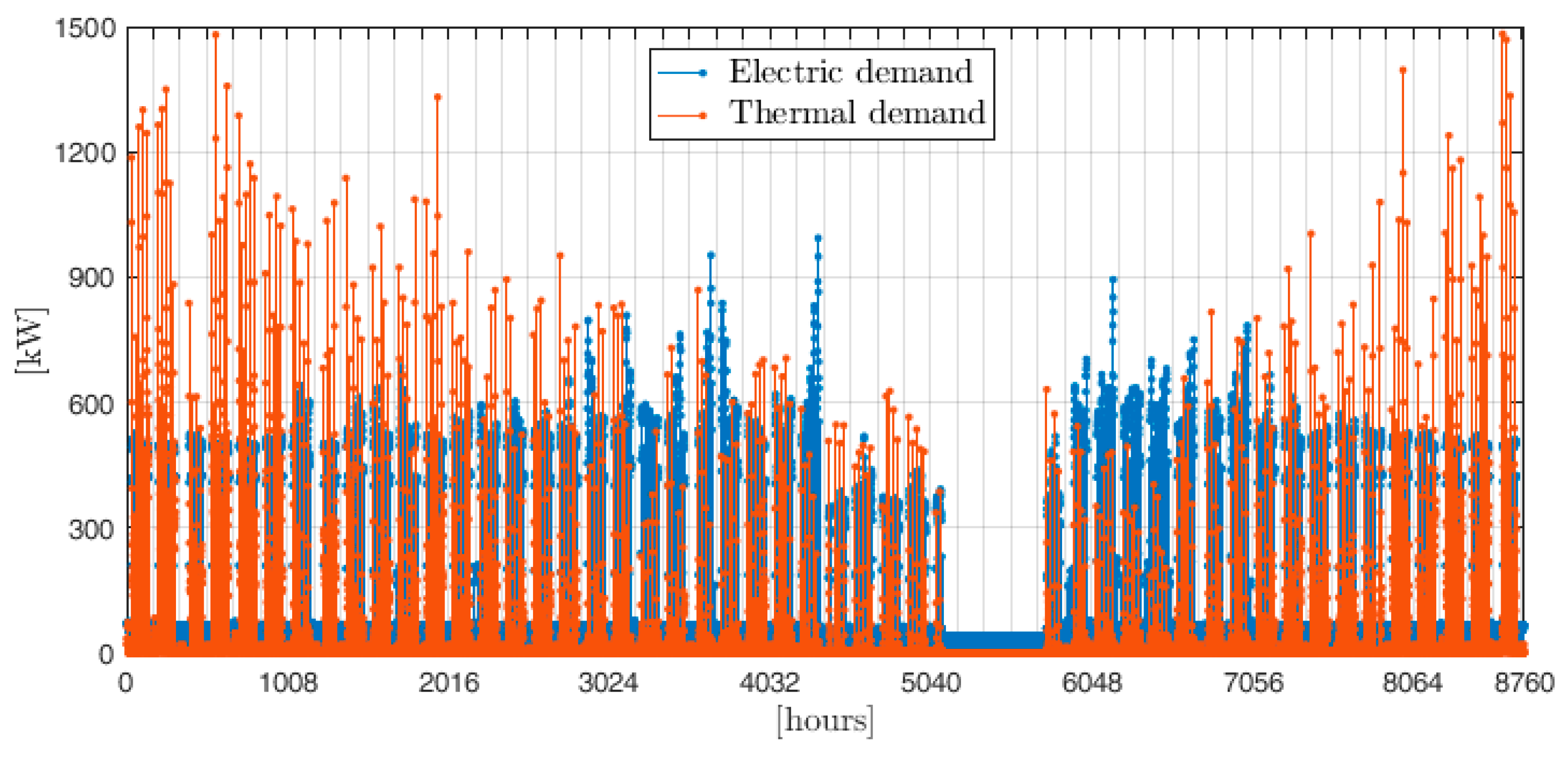
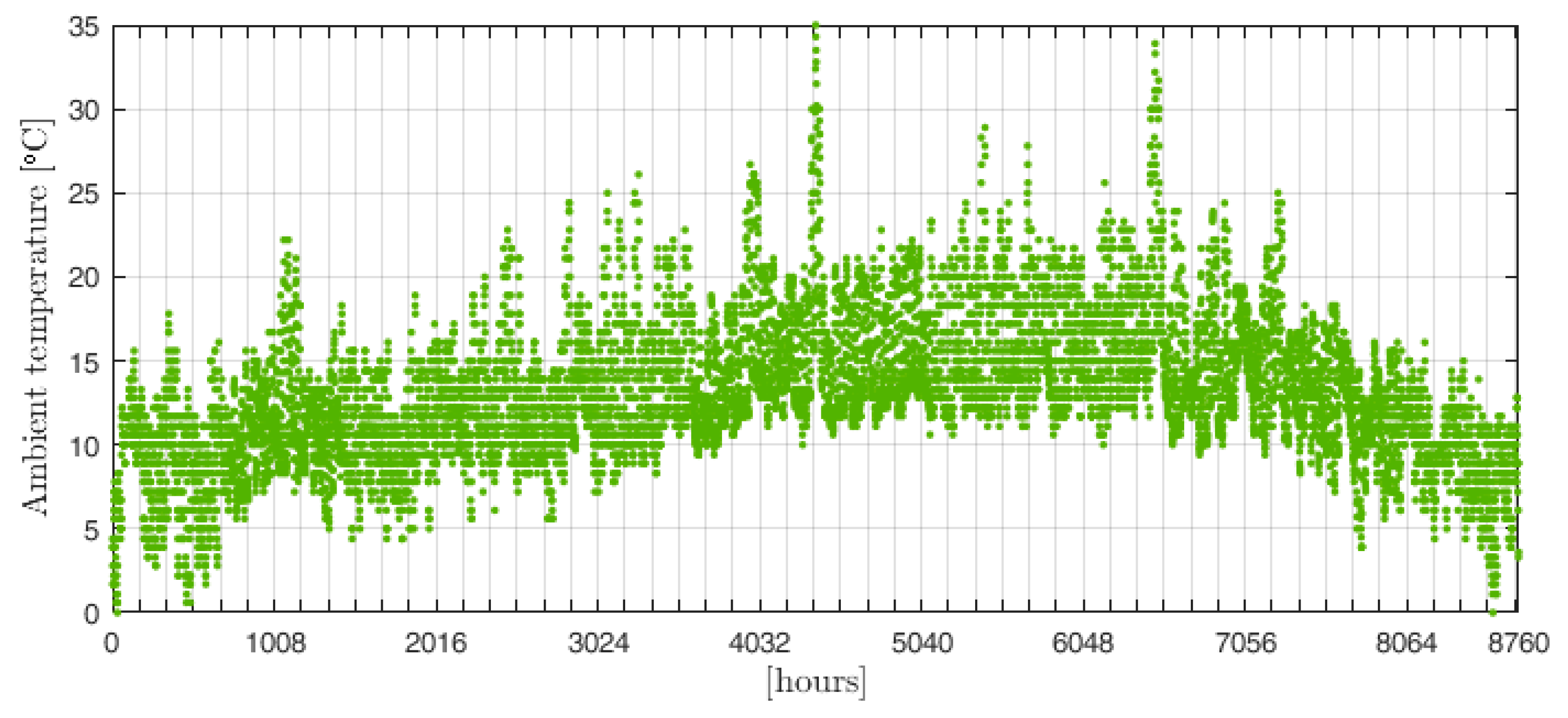
The case study used for testing the methodology was chosen from the commercial reference buildings database [26] of the US Department of Energy (DOE). A secondary school located in San Francisco (California) and constructed after the year of 1980 was selected. Data about the energy load demands (whose hourly values are shown in Figure 4) were calculated by means of EnergyPlus simulation software [27] and then imported and processed in MATLAB. Hourly temperatures of the typical meteorological year of San Francisco, which are shown in Figure 5, were considered.

3.2. The Energy System: Technical and Economic Characterization

In this section, the values of the parameters adopted to characterize the energy system optimized in the case study are shown.

Table 2. Technical characteristics and thermophysical properties.

Parameter	Value	Parameter	Value
${\eta }_{E,CHP,nom}$	$38.5\%$ [8]	${\eta }_B$	$80\%$ [28]
${\eta }_{H,CHP,nom}$	$34.4\%$ [8]	$U_{TES}$	$0.5\frac{W}{m^{2}K}$ [16]
$a_{E,CHP}$	$1.1260$ [8]	${\rho }_{TES}$	$992 \mathrm{kg}/{\mathrm{m}}^3$
$b_{E,CHP}$	$-0.1260$ [8]	$c_{TES}$	$4.186\mathrm{kJ}/\mathrm{kgK}$
$a_{H,CHP}$	$0.8253$ [8]	${\eta }_{TES,charge}$	$96\%$ [28]
$b_{H,CHP}$	$0.1747$ [8]	${\eta }_{TES,discharge}$	$96\%$ [28]

shows the technical characteristics and the thermophysical properties, while

Table 3. Prices of energy carriers and investment costs parameters.

Parameter	Value	Parameter	Value
$C_F$	$40 €/\mathrm{MWh}$ [8]	${\beta }_B$	$0.7627$ [28]
$C_{PE}$	$150\frac{€}{\mathrm{MWh}}$[8]	${\alpha }_{TES}$	$100.0$ [16]
$C_{SE}$	$50 €/\mathrm{MWh}$ [8]	${\beta }_{TES}$	$1$ [16]
${\alpha }_{CHP}$	$15460.0$ [8]	${\alpha }_{TES,charge/discharge,max}$	$800$ [19]
${\beta }_{CHP}$	$0.7247$ [8]	${\beta }_{TES,charge/discharge,max}$	$0.6$ [19]
${\alpha }_B$	$345.9$ [28]	$r$	$2\%$ [29]

summarizes the economic parameters. The lifetime was considered to be equal to 20 years for all the considered technologies.

The maximum allowed temperature of the storage was set to 95 °C, while the minimum usable temperature was 60 °C. Moreover, to minimize TES heat losses, the shape of the cylindrical tank was chosen, such as to minimize its surface. Thus, the aspect ratio was set to equal 1, and the heat-loss coefficient becomes:

$${\theta }_{TES,loss}=\frac{6U_{TES}\tau }{{\rho }_{TES}{c}_{TES}}{\left(\frac{\pi }{4V_{TES}}\right)}^{\frac{1}{3}}$$

(34)

Moreover,

Table 4. Range of values of the design variables.

Parameter	Minimum Value	Maximum Value
$P_{CHP,nom}\left[\mathrm{kW}\right]$	$200$	$1000$
$V_{TES} \left[{\mathrm{m}}^3\right]$	$0$	$50$
$Q_{B,nom} \left[\mathrm{kW}\right]$	$500$	$1500$
$Q_{TES,charge,max} \left[\mathrm{kW}\right]$	$0$	$2000$
$Q_{TES,discharge,max} \left[\mathrm{kW}\right]$	$0$	$2000$

shows the search space of the design variables in the optimization problem.

4. Results and Discussion

In this section, the results are presented as follows. First, a preliminary parametric analysis is performed to identify the value of the rolling-horizon parameters to be adopted in the optimization. Then, the proposed methodology is applied in the case study and the results are shown and discussed.

4.1. Tuning of the Rolling-Horizon Parameters

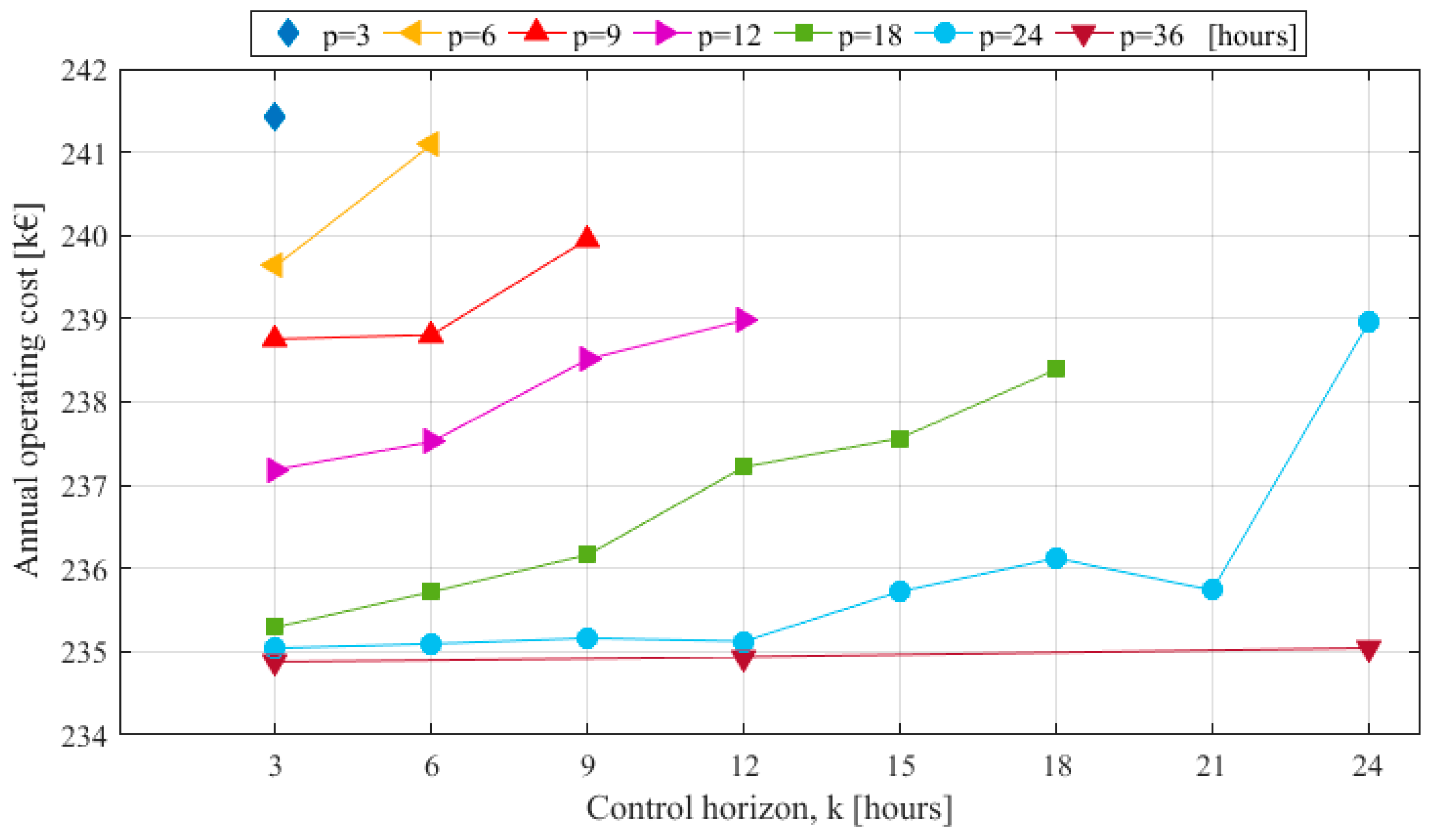
The rolling-horizon technique adopted for the decomposition of the optimal operation problem calls for the choice of the value of both the control (k) and prediction (p) horizon, which, as stated above, should be made based on a compromise between the accuracy of the solution and the computational time. Therefore, a parametric analysis aimed at assessing the impact of k and p on the annual operating cost—and consequently on the accuracy of the optimal control solution—as well as on the computational time was carried out.

To this end, several simulations were run, by varying the values of the parameters, p and k, within the range of $3-36$.

Table 5. Size of the components adopted in the rolling-horizon parametric analysis.

Parameter	$P_{CHP,nom}$	$V_{TES}$	$H_{B,nom}$	$H_{TES,charge,max}$	$H_{TES,discharge,max}$
Value	$400 \mathrm{kW}$	$50 {\mathrm{m}}^3$	$1000 \mathrm{kW}$	$2000 \mathrm{kW}$	$2000 \mathrm{kW}$

shows the size of the system components considered in this analysis. The storage capacity was chosen equal to its maximum value considered in the design stage, in order to ensure a conservative assessment of the impact of the rolling-horizon parameters on the accuracy of the solution. Indeed, it has been shown by [24] that the larger the capacity of the storage, the longer the prediction horizon should be so that the solution of the decomposed problem coincides with the solution of the original problem (i.e., the operation problem solved considering the whole-time horizon at once). In this way, when smaller storage capacities are considered in the optimal sizing problem, no deterioration of the accuracy of the solution will occur compared to that of this parametric analysis.

The results are shown in Figure 6, where the annual operating cost is reported as a function of both the control and the prediction horizon values. Once the length of the control horizon was fixed, the operating cost reduces as the prediction horizon increases, and a saturation effect can be observed. When the prediction horizon increases from 24 to 36 h, with a 3-h control horizon, the cost reduction is lower than 0.1%. Indeed, a longer prediction horizon cannot be exploited because of the limited capacity of the storage. On the other hand, for a given value of p, the operating cost increases as the control horizon increases. Nonetheless, with p equal to 24 h, no relevant differences are observed when k ranges from 3 to 12 h. In fact, if the prediction horizon is long enough, longer control horizons can be adopted, thus reducing the overall number of the optimization sub-problems. Therefore, the values of k = 12 and p = 24 were chosen, since these values represent a good compromise between the solution accuracy and the computational time.

4.2. Optimization Results

Table 6. Results from case-study optimization.

Parameter	Value	Parameter	Value
$P_{CHP,nom}$	$400 \mathrm{kW}$	$Q_{TES,discharge,max}$	$425 \mathrm{kW}$
$V_{TES}$	$12.5 {\mathrm{m}}^3$	$EAC$	$317.9 \mathrm{k}€$
$Q_{B,nom}$	$1000 \mathrm{kW}$	$O$	$237.7 \mathrm{k}€$
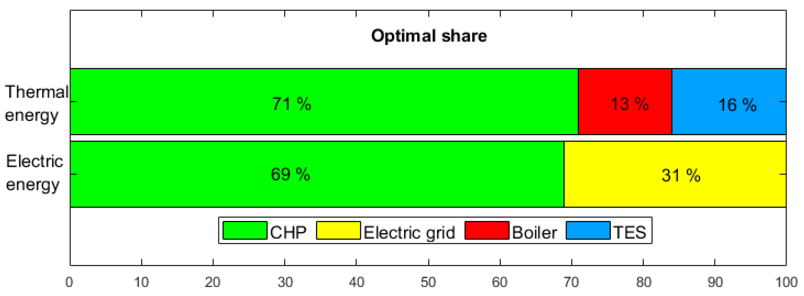
$Q_{TES,charge,max}$	$275 \mathrm{kW}$	$I$	$80.2 \mathrm{k}€$

summarizes the main results from the optimization. The optimal size of each component as well as the hourly optimal operation throughout the year were identified. In Figure 7, the annual electric and thermal load shares for the optimal configuration are shown. Both the electric and thermal annual demand are directly met by the CHP for around 70%, while the TES contributes 16% to cover the heat demand.

Figure 8, Figure 9 and Figure 10 show examples of how the optimized energy system works and what kind of detailed outputs are available from the simulations. Figure 8 shows how the electric demand is met in a typical week. During the day, the CHP operates at full load, covering an average of 80% of the electric demand, while the remaining demand is met by purchasing electricity from the grid. During the night and the weekend, the CHP is generally off, since the electric demand is lower than its minimum capacity, and the electricity is bought from the grid. It is interesting to note that the optimal operation entails a very limited exchange with the power grid, thus avoiding stressing the stability and management of the electricity network.

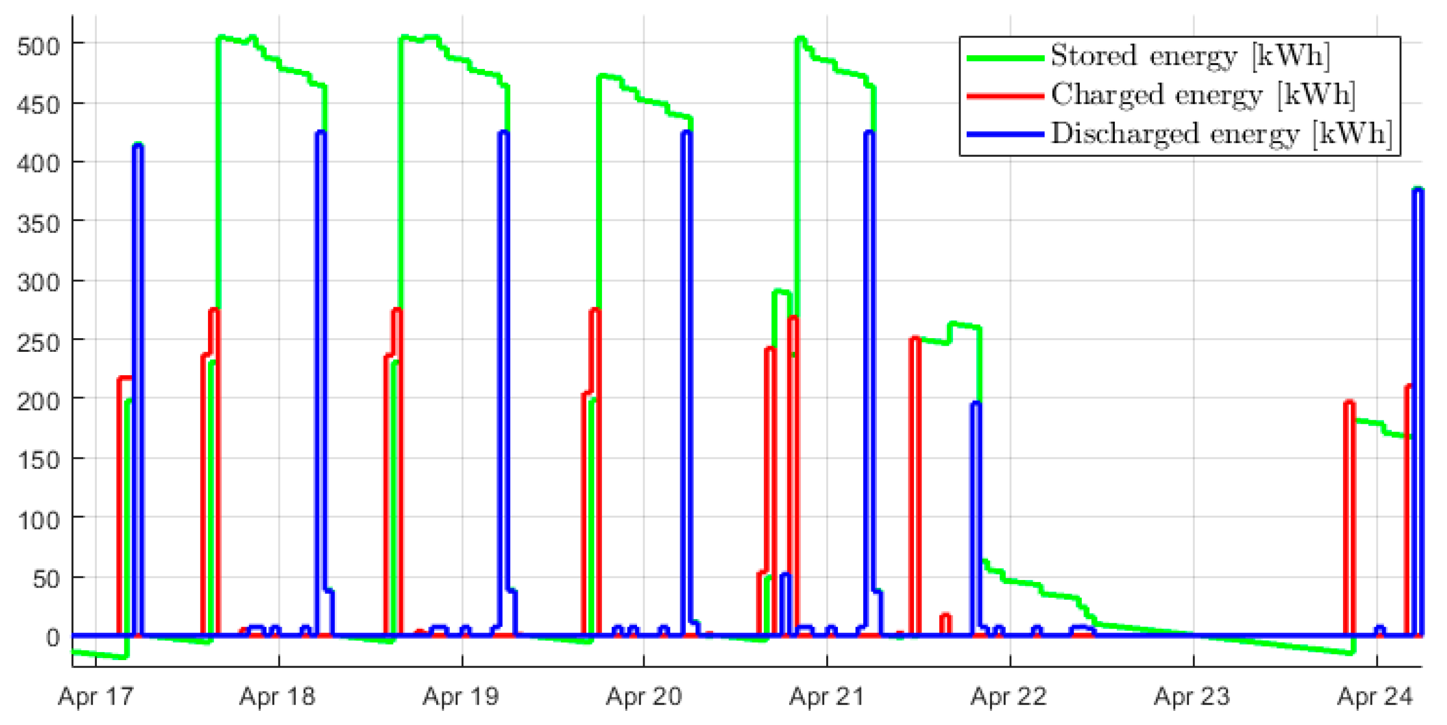
Figure 9 shows the same kind of results for the thermal demand. The CHP production completely covers the demand for most of the week, except when the morning peak demands occur. In those cases, the storage is discharged, and the boiler meets the remaining heat demand. On the other hand, in the evening, before the CHP is turned off, the TES is charged so that thermal energy is available in the morning. This behavior can be clearly seen in Figure 10.

As a result, the scheduling of the CHP is mainly driven by the electric demand, while the thermal output of the CHP unit is generally larger than the heat demand. Nonetheless, the thermal storage allows a fraction of the exceeding CHP thermal production to be saved, which is used to shave the heat peak demand in the early hours of the morning, when the start up of the whole heating distribution and emission system occurs. In this way, the boiler production is minimized, even though the heat capacity of the CHP is well below the thermal peak demand.

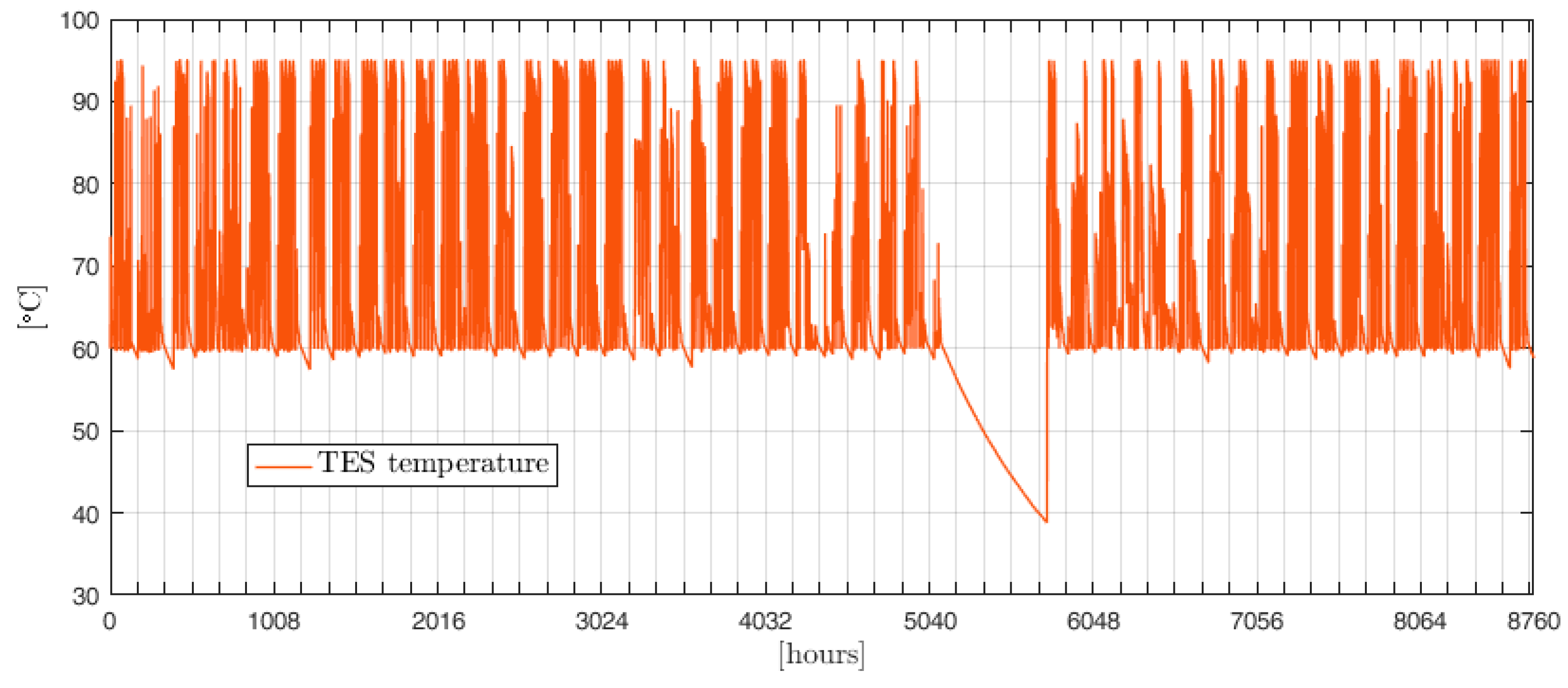
Finally, Figure 11 shows how the equivalent temperature of the storage varies throughout the year. Most of the time, its value fluctuates between 95 °C, when the storage is fully charged, and 60 °C, when the storage has just been completely discharged. Moreover, during the weekends, when there is no usage of the storage, the equivalent temperature drops below 60 °C as a result of the heat losses. This behavior is particularly emphasized during the month of August, when the school is closed and there is no thermal demand for a long period. Thus, it is more convenient to let the storage discharge due to thermal losses, rather than maintaining it at the usable temperature. As already explained, traditional approaches do not allow this behavior to be obtained, and thanks to the proposed formulation, a more comprehensive simulation of the TES has been enabled.

5. Conclusions

A comprehensive methodology for the optimal design of cogeneration systems with integrated thermal energy storage was proposed in this paper. The integrated optimization problem of the sizing of the equipment and operational strategy was decomposed into two levels to take into account the part-load behavior of the cogeneration unit, variation of the unitary cost of the components in relation to their size, and the effect of the storage volume on its thermal losses. The optimal operation problem was formulated so as to exploit mixed integer linear programming solvers, while the optimal sizing was tackled by means of a genetic algorithm.

A novel mixed integer linear formulation for the thermal energy storage was proposed. Both “static” and “dynamic” heat losses were considered, and the heat-loss coefficient was defined as a function of the geometrical and thermophysical properties of the storage. The introduction of a binary variable allowed a more comprehensive simulation of the operation of the storage. Furthermore, a rolling-horizon procedure was presented to reduce the computational time of the optimization problem, while preserving the quality of the results.

The methodology was tested in a case study, namely a secondary school located in San Francisco, California. The optimal size and operation of the cogeneration system with thermal energy storage were identified. Results from the optimization were presented and discussed. A parametric analysis led to the identification of the optimal values of the rolling-horizon parameters: 24 h for the prediction horizon and 12 h for the control horizon were chosen as a compromise between the accuracy of the results and the computational time. In the case study, the cogeneration unit directly covers around 70% of both the electric and thermal annual demand, while 16% of the latter is met by the storage.

Moreover, the results showed how the proposed formulation allows control strategies for the thermal energy storage to be exploited that cannot be taken into account with conventional simplified formulations. Indeed, instead of keeping the state of charge of the storage always above its minimum operational threshold, the controller allows it to drop below its threshold value. This behavior is particularly marked during extended periods of low or nil demand, as in August, when the school is closed and the temperature of the storage drops significantly below its operational threshold.

Future research may focus on: More complex multi-energy systems (modular cogeneration, heat pumps, renewable energy technologies), the effect of uncertainties on the optimal design, and multi-objective optimization with further criteria (environmental, energetic, exergetic indicators).

References

- Isa, N.M.; Tan, C.W.; Yatim, A.H.M. A comprehensive review of cogeneration system in a microgrid: A perspective from architecture and operating system. Renew. Sustain. Energy Rev. 2018, 81, 2236–2263. [Google Scholar] [CrossRef]
- Gimelli, A.; Muccillo, M. The key role of the vector optimization algorithm and robust design approach for the design of polygeneration systems. Energies 2018, 11. [Google Scholar] [CrossRef]
- Zhang, G.; Cao, Y.; Cao, Y.; Li, D.; Wang, L. Optimal energy management for microgrids with combined heat and power (CHP) generation, energy storages, and renewable energy sources. Energies 2017, 10, 1288. [Google Scholar] [CrossRef]
- Franco, A.; Versace, M. Optimum sizing and operational strategy of CHP plant for district heating based on the use of composite indicators. Energy 2017, 124, 258–271. [Google Scholar] [CrossRef]
- Gimelli, A.; Muccillo, M.; Sannino, R. Optimal design of modular cogeneration plants for hospital facilities and robustness evaluation of the results. Energy Convers. Manag. 2017, 134, 20–31. [Google Scholar] [CrossRef]
- Beihong, Z.; Weiding, L. An optimal sizing method for cogeneration plants. Energy Build. 2006, 38, 189–195. [Google Scholar] [CrossRef]
- Aviso, K.B.; Tan, R.R. Fuzzy P-graph for optimal synthesis of cogeneration and trigeneration systems. Energy 2018, 154, 258–268. [Google Scholar] [CrossRef]
- Urbanucci, L.; Testi, D. Optimal integrated sizing and operation of a CHP system with Monte Carlo risk analysis for long-term uncertainty in energy demands. Energy Convers. Manag. 2018, 157. [Google Scholar] [CrossRef]
- Yokoyama, R.; Takeuchi, S.; Ito, K. Thermoeconomic analysis and optimization of a gas turbine cogeneration units by a systems approach. In Proceedings of the ASME Turbo Expo, Barcelona, Spain, 6 May 2006. [Google Scholar]
- Fang, T.; Lahdelma, R. Optimization of combined heat and power production with heat storage based on sliding time window method. Appl. Energy 2016, 162, 723–732. [Google Scholar] [CrossRef] [Green Version]
- Kuang, J.; Zhang, C.; Li, F.; Sun, B. Dynamic Optimization of Combined Cooling, Heating, and Power Systems with Energy Storage Units. Energies 2018, 11, 2288. [Google Scholar] [CrossRef]
- Elsido, C.; Bischi, A.; Silva, P.; Martelli, E. Two-stage MINLP algorithm for the optimal synthesis and design of networks of CHP units. Energy 2017, 121, 403–426. [Google Scholar] [CrossRef]
- Fuentes-Cortés, L.F.; Ponce-Ortega, J.M.; Nápoles-Rivera, F.; Serna-González, M.; El-Halwagi, M.M. Optimal design of integrated CHP systems for housing complexes. Energy Convers. Manag. 2015, 99, 252–263. [Google Scholar] [CrossRef]
- Urbanucci, L. Limits and potentials of Mixed Integer Linear Programming methods for optimization of polygeneration energy systems. Energy Procedia 2018, 148, 1199–1205. [Google Scholar] [CrossRef]
- Marquant, J.F.; Evins, R.; Carmeliet, J. Reducing computation time with a rolling horizon approach applied to a MILP formulation of multiple urban energy hub system. Procedia Comput. Sci. 2015, 51, 2137–2146. [Google Scholar] [CrossRef]
- Steen, D.; Stadler, M.; Cardoso, G.; Groissböck, M.; DeForest, N.; Marnay, C. Modeling of thermal storage systems in MILP distributed energy resource models. Appl. Energy 2015, 137, 782–792. [Google Scholar] [CrossRef] [Green Version]
- Combined Heat and Power & Trigeneration Solutions, Wartsila. Available online: https://www.wartsila.com/docs/default-source/power-plants-documents/downloads/brochures/chp-2017.pdf?sfvrsn=6c60f145_4 (accessed on 31 January 2019).
- Omu, A.; Hsieh, S.; Orehounig, K. Mixed integer linear programming for the design of solar thermal energy systems with short-term storage. Appl. Energy 2016, 180, 313–326. [Google Scholar] [CrossRef]
- Bejan, A.; Tsatsaronis, G.; Moran, M. Thermal Design and Optimization, 1st ed.; Wiley India: New Delhi, India, 1995. [Google Scholar]
- IBM ILOG CPLEX Optimizer. Available online: http//www-01.ibm.com/software/integration/Optim (accessed on 30 December 2018).
- MATLAB Genetic Algorithm Solver. Available online: https://it.mathworks.com/discovery/genetic-algorithm.html (accessed on 30 December 2018).
- Ommen, T.; Markussen, W.B.W.B.; Elmegaard, B. Comparison of linear, mixed integer and non-linear programming methods in energy system dispatch modelling. Energy 2014, 74, 109–118. [Google Scholar] [CrossRef]
- Bischi, A.; Taccari, L.; Martelli, E.; Amaldi, E.; Manzolini, G.; Silva, P.; Campanari, S.; Macchi, E. A rolling-horizon optimization algorithm for the long term operational scheduling of cogeneration systems. Energy 2018. [Google Scholar] [CrossRef]
- D’Ettorre, F.; Conti, P.; Schito, E.; Testi, D. Model predictive control of a hybrid heat pump system and impact of the prediction horizon on cost-saving potential and optimal storage capacity. Appl. Therm. Eng. 2019, 148, 524–535. [Google Scholar] [CrossRef]
- Urbanucci, L.; Testi, D.; Bruno, J.C. An operational optimization method for a complex polygeneration plant based on real-time measurements. Energy Convers. Manag. 2018, 170. [Google Scholar] [CrossRef]
- Office of Energy Efficiency and Renewable Energy. Commercial Reference Buildings. Available online: https://www.energy.gov/eere/buildings/commercial-reference-buildings (accessed on 30 December 2018).
- EnergyPlus Simulation Software. Available online: https://energyplus.net (accessed on 30 December 2018).
- Marquant, J.F.; Evins, R.; Bollinger, L.A.; Carmeliet, J. A holarchic approach for multi-scale distributed energy system optimisation. Appl. Energy 2017, 208, 935–953. [Google Scholar] [CrossRef] [Green Version]
- Vögelin, P.; Koch, B.; Georges, G.; Boulouchos, K. Heuristic approach for the economic optimisation of combined heat and power (CHP) plants: Operating strategy, heat storage and power. Energy 2017, 121, 66–77. [Google Scholar] [CrossRef]
Figure 1.
Schematic representation of the combined heat and power system.
Figure 2.
Outline of the bi-level optimization algorithm.
Figure 3.
Rolling-horizon approach.
Figure 4.
Energy load demand of the case study.
Figure 5.
Hourly ambient temperature for the case study [27].
Figure 6.
Impact of the prediction and control horizon lengths on the annual operating cost.
Figure 7.
Optimal electric and thermal load sharing.
Figure 8.
Optimal operation: electric demand and load sharing in a typical week.
Figure 9.
Optimal operation: thermal demand and load sharing in a typical week.
Figure 10.
Optimal operation: TES stored, charged, and discharged energy in a typical week.
Figure 11.
Hourly equivalent TES temperature during the year.