Article

Permanent-Magnet Synchronous Motor Sensorless Control Using Proportional-Integral Linear Observer with Virtual Variables: A Comparative Study with a Sliding Mode Observer

School of Electrical Engineering and Automation, Harbin Institute of Technology, Harbin 150001, China
*
Authors to whom correspondence should be addressed.
Energies 2019, 12(5), 877; https://doi.org/10.3390/en12050877
Submission received: 15 January 2019 / Revised: 16 February 2019 / Accepted: 28 February 2019 / Published: 6 March 2019
(This article belongs to the Special Issue Control in Power Electronics)

Abstract

:
Quick convergence, simple implementation, and accurate estimation are essential features of realizing permanent-magnet synchronous motor (PMSM) position estimation for sensorless control using microcontrollers. A linear observer is often designed on real plant variables and is more sensitive to parameter uncertainty/variations. Thus, conventionally, a sliding mode observer (SMO)-based technique is widely used for its simplicity and convergence ability against parameter uncertainty. Although SMO has been improved for switching chattering and phase delay, it provides purely proportional gain, which leads to steady-state error and chattering in observation results. Different from conventional linear observer using real plant variables or SMO with proportional gain, a simple proportional-integral linear observer (PILO) using virtual variables is proposed in this paper. This paper also provides a comparative study with SMO. By introducing virtual variables without physical meaning, the PILO is able to simplify observer relations, get smaller phase shifts, adapt mismatched parameters, and obtain a fixed phase-shift relation. The PILO is not only simple, but also improves the estimation precision by solving the controversy between chattering and phase-delay, steady-state error. Moreover, the PILO is less sensitive to parameters mismatching. Simulation and experimental results indicate the merits of the PILO technique.

1. Introduction

Permanent magnet synchronous machine (PMSM) has been widely used in industrial applications that require high precision or high efficiency, such as automation production lines, electric vehicles, robots, and wind turbines. The PMSM sensorless control techniques can be mainly classified in two groups: model-saliency-dependent techniques and model-dependent techniques.
In the first group, rotor position is usually detected by measuring the response signals, which are induced from high-frequency signals injected in windings [1,2,3,4]. However, signal injection can cause torque ripple, increase power loss, and decrease available voltage for the motor drive. Moreover, the signal injection technique is not suitable for surface-mounted PMSM (SPMSM) applications. Additionally, secondary saliency-like cross-saturation and higher harmonic saliency coupling can also degrade the position estimation precision.
In the second group, position-related-variables, such as flux, back electromotive force (EMF), or speed, can be obtained using motor model-dependent tools (such as observer [5,6,7], model reference method [8,9], etc.) with known model input and some measurable state variables. In the extremely high speed range, the iron loss is not negligible for back EMF estimation, which can be compensated for using a look-up table [5]. As an open-loop voltage/frequency (V/F) or current/frequency (I/F) start-up can be used for a low speed range, a back EMF observation technique is widely adopted in industrial applications, such as fans and pumps, which works in the medium to high speed range and do not suffer from heavy load torque during startup.
To obtain back EMF, different observers are adopted. The Kalman filter observer [6,10,11] is limited due to its demand of computation resources for the matrix calculations. Luenberger observer [12] and disturbance observer convergence speeds are less than non-linear observers. Besides, conventional linear observers are based on real plant variables, resulting in sensitivity on parameter variation. As revealed in Reference [13], the use of real plant variable can induce observation errors on two levels: the parameter mismatch level and the observer dynamic level. Given these circumstances, the sliding mode observer is widely used because of its simplicity and robustness [14,15,16,17].
However, the conventional SMO suffers from a chattering problem because of discrete switching control function. The conventional solution of introducing one or several low-pass filters can increase the phase delay. Both chattering and phase delay can result in estimation error, which will decrease control accuracy, cause extra power loss, or even cause instability during the dynamic process. Different approaches have been proposed to handle the chattering problem. Chattering can be reduced using a sigmoid function [16,18]. A sigmoid function improved with a variable boundary for different speed range is also reported [19]. After having obtained a back EMF signal, a synchronous frequency filter (SFF) is reported to filter out the chattering high frequency oscillation [20]. Extracting the position signal using a phase-lock-loop (PLL) [20,21] also gives improved chattering than a trigonometric function.
In the above observing solutions, either conventional SMO or improved SMO eventually provides purely proportional gain, although non-linear. The proportional gain can result in a steady-state error for estimation. Increasing the gain leads to less steady-state error, but the oscillation of position estimation can be enlarged.
Different from a conventional linear observer using real plant variable or SMO using proportional gain, a simple proportional-integral linear observer (PILO) using virtual variables is proposed in this paper. This paper also provides a comparative study with SMO. By introducing two virtual variables without physical meaning, the PILO is able to get a smaller phase shift, adapt mismatched parameters, and obtain a fixed phase-shift relation. The PILO is not only simple, but also improves the estimation precision by solving the controversy between chattering and phase-delay, steady-state error. Moreover, the PILO is less sensitive to parameters mismatching. Simulation and experimental results indicate the merits of PILO technique.
This paper is organized as follows: The PMSM model is given in Section 2. In Section 3, the drawbacks of SMO and the proposed PILO are given. Section 4 provides simulation and experimental results. Section 5 concludes this paper.

2. PMSM Model and Control Structure

2.1. PMSM Continuous-Time Model

The mathematical model of an SPMSM can be described in the stationary α β reference frame as follows:
d d t i s = Φ i s + Γ u s Γ e s
and
e s = ω e ψ m [ sin θ e cos θ e ]
where i s = [ i α , i β ] T , u s = [ u α , u β ] T , e s = [ e α , e β ] T , Φ = R s L s I 2 , Γ = 1 L s I 2 , and I 2 is a 2 × 2 identity matrix. The bold symbols in the equations represent a vector or matrix. Variables i α , i β ; u α , u β ; and e α , e β are phase currents, phase voltages, and back EMF in the stationary α β reference frame, respectively. L s and R s are stator inductance and stator resistance, ω e is electrical angular velocity, θ e is electrical rotor position, and ψ m is the flux linkage using permanent magnets.

2.2. Discrete-Time Model

In the stationary reference frame, the structure of current functions in the α -axis and β -axis are the same. By using zero-order hold discretization methods, and using the index k to indicate a corresponding discrete value at the time instant t = k T , Equation (3) can be obtained from Equation (1):
I ( k ) = A I ( k 1 ) + B U ( k ) B E ( k )
where
A = e R s L s T I 2 B = 1 R s ( 1 e R s L s T ) I 2
with T being the sampling period and e being the natural constant.

2.3. Sensorless Control Structure

Figure 1 shows the block diagram of a sensorless vector control with an observer. Conventional i * d = 0 field-oriented control is used for a PMSM drive, and the position observation is implemented in the αβ reference frame. i * d is the reference for the d-axis current control.
The drawbacks of conventional SMO and the analysis of PILO is compared in the subsequent section.

3. Comparison of SMO and PILO

This section starts with the analysis of the drawbacks of conventional SMO, and then the proposed PILO is given in continuous and discrete form with analysis.

3.1. SMO and Its Drawbacks

In this part, a widely used SMO in engineering is analyzed. This SMO has an integrated filter to reduce chattering. The drawbacks are analyzed as follows.
Equation (1) is extended to:
{ d d t i s = Φ i s + Γ ( u s e s ) d d t x s = 0
where x s always takes the value of zero.
The back EMF estimation contains high frequency noise due to sliding mode switching. A satisfactory filtering of the signal can result in a large phase delay. One solution is to use both filtered and switching signals, where the SMO with a filter is as follows:
{ d d t i ^ s = Φ i ^ s + Γ ( u s z z f ) z = k sgn ( i ^ s i s ) d d t z f = ω z ω z f
Usually, the estimated back EMF takes the value as follows:
e ^ s = 2 z f
Subtracting Equation (5) from Equation (6) yields:
{ e 1 = i ^ s i s e 2 = z f x s e ˙ 1 = Φ e 1 + Γ ( e s z z f ) e ˙ 2 = ω z ω z f
In a steady state, e ˙ 1 = 0 and e ˙ 2 = 0 should be satisfied, thus:
{ z = z f e 1 = Φ 1 Γ ( z + z f e s ) = Φ 1 Γ ( 2 z e s ) e 2 = z
It can be seen that e 2 equals to z in a steady state, instead of the real EMF e s precisely. z is obtained from a combination of proportional gain and the sign function. Note x s always takes the value of zero. Therefore, e ^ s = 2 e 2 . Thus:
{ e ^ s = 2 k i f   e 1 > 0 e ^ s = 2 k i f   e 1 < 0
It can be seen that in one state, the EMF observation can only converge to the gain value other than the real EMF value, where an estimation error exists. In fact, to ensure the sliding mode works, it should be large enough, as k > max ( | e α | , | e β | ) . In this case, when reaching one steady state, where the EMF is overestimated according to the k definition, the current estimation i ^ s will decrease and result in the other “steady state.” The single steady state cannot persist, which is the cause of chattering. To sum up, two main inherent drawbacks of ESO, estimation error and chattering, are unavoidable, even with filters. When the parameters of SMO are inappropriate, chopping and error become more serious.

3.2. Continuous-Time Model of the Proposed PILO

In order to estimate the back EMF in the stationary reference frame with integral gain, the observer equation of PILO is given as:
d d t y s = Φ y s + Γ u s Γ Q s
where y s = [ y α , y β ] T , which has no physical meaning and is a virtual variable to establish the PILO and to simplify the observer relation. Q s is a normal linear equation for introducing integral gain to the observer. The equation is:
Q s = l 1 x s + l 2 x ˙ s
and the variables x s are defined as the integral of x ˙ s , and x ˙ s is given by Equation (13):
x ˙ s = y s i s
For observation error analysis, Equation (1) is subtracted from Equation (11), and the difference equation is obtained as in Equation (14):
x ¨ s = Φ x ˙ s + Γ e s Γ Q s
Equation (14) including x s and e s can be written with a second-order transfer function, as in Equation (15):
x s ( s ) e s ( s ) = ω 0 2 s 2 + 2 ζ ω 0 s + ω 0 2 1 l 1
where
ω 0 2 = l 1 L s ζ = ( R s + l 2 ) / L s 2 ω 0
Let the estimated back EMF e ^ s take the form as follows:
e ^ s = l 1 x s
ω 0 represents the observer bandwidth. In this paper, the damping ratio ζ takes the value of 1. Then, the transfer function is:
e ^ s ( s ) e s ( s ) = ω 0 2 ( s + ω 0 ) 2
This transfer function is second order, which does not suffer from chattering and steady-state error. By introducing the virtual variable, the observer relation is simplified.

3.3. Discrete-Time Model of PILO

The discrete-time model of Equations (11), (12), and (13) is given as:
Y ( k ) = A Y ( k 1 ) + B U ( k ) B Q ( k ) X 2 ( k ) = Y ( k ) I ( k ) X 1 ( k ) = X 2 [ ( k 1 ) ] + T X 2 ( k ) Q ( k ) = L 1 X 1 ( k 1 ) + L 1 X 2 ( k 1 )
where Y ( k ) , U ( k ) , Q ( k ) , X 1 ( k ) , and X 2 ( k ) are the discrete signals of y s , u s , Q s , x s , and x ˙ s , respectively.
According to Equation (17) the estimated back EMF E ^ ( k ) , i.e., [ e α e β ] T , is as follows:
E ^ ( k ) = L 1 X 1 ( k )
The observer parameter has to be fixed. By discretizing the transfer function Equation (18) using zero-order hold methods, Equation (21) can be obtained:
E ^ ( z ) E ( z ) = [ z T ω 0 ( 1 e ω 0 T ) ( z e ω 0 T ) 2 ]
L 1 and L 2 can be calculated through Equations (19)–(21) as Equation (22):
L 1 = R s ( 1 e ω 0 T ) 2 T s ( 1 e R s L s T ) I 2 L 2 = R s ( e R s L s T + 1 2 e ω 0 T ) ( 1 e R s L s T ) I 2
The estimated electrical angular position is as follows:
θ ^ e ( k ) = tan 1 ( E α * ( k ) E β * ( k ) ) δ ( k )
where θ ^ e is the estimated value of the electrical rotor position θ e . δ is the compensation of the steady-state phase shift produced by the observer.
The inputs of transform function Equation (18), e α and e β , are trigonometric functions, and δ ( k ) can be calculated as:
δ ( k ) = tan 1 ( 2 ( ω ^ e ( k ) / ω 0 ) 1 ( ω ^ e ( k ) / ω 0 ) 2 )
where ω ^ e is the estimated electrical angular velocity.

4. Results and Discussion

This section gives the performance comparison of the PILO and SMO. The comparison involves performance in the steady-state, transient-state, and parameter mismatch cases.
Table 1 shows the tested motor parameters. The parameters of the two observers are given in Table 2 and Table 3, respectively.
In an actual situation, the parameters of the motor have uncertainties. The mismatched parameter influence is also evaluated. The mismatched parameters used in observers are given in Table 4.

4.1. Simulation Results

In the simulation, the load of motor was set from 0 to 1 Nm at 0.15 s. In order to ensure good performance of the SMO with less chattering, the SMO gain k was adjusted according to the speed of the motor, which satisfied k > max ( | e α | , | e β | ) to ensure the convergence of the EMF estimation with switching. The higher the motor speed, the greater the value of the gain k .
The phase delay was compensated. For the PILO, the phase delay δ was calculated and compensated for using Equation (24). For SMO, the phase delay was tuned manually for different speeds. The phase delay is further discussed in experimental results.
Figure 2 shows the dynamic performance of the two observers. For the PILO, as in Figure 2a, the position error was less than 0.2% throughout the test. Figure 2b shows the performance of the SMO. The position error was less than 0.6%. In Figure 2b, the required SMO gain was larger when the motor rotated faster. Therefore, the chattering problem was more serious at high speeds. In simulation, where current measurement was ideal (without noise and filter), the SMO chattering was caused by sliding mode switching. Low gain values gave lower chattering, which resulted in better performance at low speeds.
Figure 3 gives the dynamic performance of the two observers with the mismatched parameters used in the observer, as given in Table 4. The motor parameters remained unchanged. For the PILO, as in Figure 3a, the position error was less than 0.7%. Figure 3b shows the performance of the SMO. The position error was less than 5%. Comparing Figure 2 and Figure 3, the performance of SMO and PILO were both influenced by the parameters mismatching. Comparing Figure 3a,b, the PILO performance was better than SMO when the motor parameters were mismatched.

4.2. Experimental Results

The observers and sensorless vector control algorithm was implemented in a TI TMS320F28069. The experimental setup is shown in Figure 4. It consisted of a DSP (Digital signal processor)-based control board, power stage, and a PMSM motor equipped with a resolver. The data was collected through the JTAG (Joint Test Action Group) communication. The two observers were compared under no-load and load conditions.
As aforementioned, the phase error was compensated during the test. For the PILO, the phase delay δ was calculated and compensated for using Equation (24). For SMO, the phase delay was tuned manually for different speeds. The phase delay is compared later in the following part.
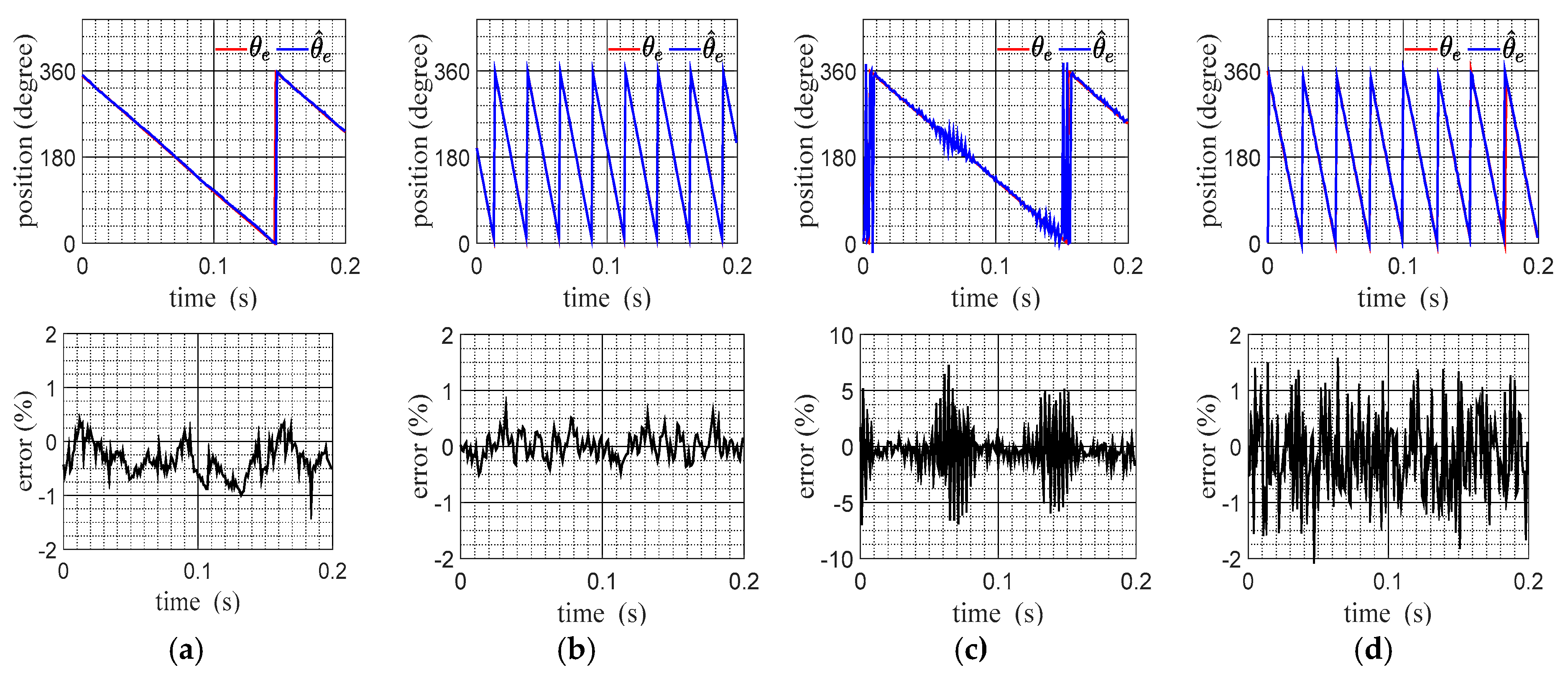
Figure 5 and Figure 6 give the performance with appropriate observer parameters under no-load and load conditions, respectively. With mechanical speeds of 100 and 600 rpm, it can be seen in the case of appropriate parameters that the loading conditions do not affect the estimation error too much. Due to current measurement noise in practical conditions, the SMO at a low speed condition did not provide less chattering than higher speed as given in simulation. Whether using loading or not, the PILO did not have chattering problems and the estimation errors were smaller.
Figure 7 and Figure 8 give the performance with mismatched observer parameters under no-load and load conditions, respectively. For the PILO, the estimation errors under no-load and load conditions are within ±1%, signifying that the mismatched parameter influence was not obvious. For the SMO, especially for low speed conditions with load, the estimation error was about ±7%, as given in Figure 8c, which was more than three times the no-loading case in Figure 7c. Besides, large oscillations could be seen. Compared with PILO, the SMO was more sensitive for parameter mismatch in a low-speed loading condition. The result is consistent with the simulation results.
As aforementioned, the PILO phase delay δ was calculated using Equation (24), and the SMO phase delay σ was manually adjusted. The two-phase compensations were compared in Figure 9 for different speeds. It was shown that phase delay of PILO was also smaller than conventional SMO. Moreover, the compensation of PILO was much simpler as it did not require extra tuning effort performed with extra tests. From the test results, it can be seen that the compensation using Equation (24) works well with only a small steady-state error less than 1%, which is acceptable.

5. Conclusions

This paper has proposed a PILO observer using a virtual variable and has given a comparative study of PMSM sensorless control using SMO and PILO. Unlike an SMO based on pure proportional gain, the PILO worked with proportional integral gain by using a virtual variable. Moreover, by introducing a virtual variable, the whole observer relation could be simplified, it was also able to get smaller phase shift, adapt mismatched motor parameters, and obtain a fixed phase relation, as indicated by experimental results.
The PILO is simple because it has only one bandwidth parameter to tune, and phase-delay compensation is easy. The PILO has good dynamic and steady-state performance. Compared with SMO, it does not suffer from a chattering problem, and it is less sensitive to mismatched parameters. The superiority of the observer has been indicated through simulation and experiment.

Author Contributions

Conceptualization, B.W.; investigation, Y.W.; validation, L.F. and J.H.; formal analysis, S.J. and Q.W.

Funding

This research was funded by the National Natural Science Foundation of China, grant number 51607045, and the Heilongjiang Postdoctoral Fund, under Grant LBH-Z15067.

Conflicts of Interest

The authors declare no conflict of interest.

References

  1. Suzuki, T.; Shimizu, Y.; Iwaji, Y.; Takahata, R.; Aoyagi, S. Minimum Current Start-Up Method by Combined Use of Two Position-Sensorless Controls. IEEE Trans. Ind. Appl. 2015, 51, 3086–3093. [Google Scholar] [CrossRef]
  2. Kim, D.; Kwon, Y.C.; Sul, S.K.; Kim, J.H.; Yu, R.S. Suppression of Injection Voltage Disturbance for High-Frequency Square-Wave Injection Sensorless Drive with Regulation of Induced High-Frequency Current Ripple. IEEE Trans. Ind. Appl. 2016, 52, 302–312. [Google Scholar] [CrossRef]
  3. Zaim, S.; Nahid-Mobarakeh, B.; Meibody-Tabar, F. Robust Position Sensorless Control of Nonsalient PMSM at Standstill and Low Speeds. IEEE J. Emerg. Select. Top. Power Electron. 2014, 2, 640–650. [Google Scholar] [CrossRef]
  4. Chen, J.-Y.; Yang, S.-C.; Tu, K.-H. Comparative Evaluation of a Permanent Magnet Machine Saliency-Based Drive with Sine-Wave and Square-Wave Voltage Injection. Energies 2018, 11, 2189. [Google Scholar] [CrossRef]
  5. Kim, J.; Jeong, I.; Nam, K.; Yang, J.; Hwang, T. Sensorless Control of PMSM in a High-Speed Region Considering Iron Loss. IEEE Trans. Ind. Electron. 2015, 62, 6151–6159. [Google Scholar] [CrossRef]
  6. Quang, N.K.; Hieu, N.T.; Ha, Q.P. FPGA-Based Sensorless PMSM Speed Control Using Reduced-Order Extended Kalman Filters. IEEE Trans. Ind. Electron. 2014, 61, 6574–6582. [Google Scholar] [CrossRef]
  7. Hu, K.W.; Liaw, C.M. Position sensorless surface-mounted permanent-magnet synchronous generator and its application to power DC microgrid. IET Power Electron. 2015, 8, 1636–1650. [Google Scholar] [CrossRef]
  8. Teja, A.V.R.; Chakraborty, C.; Maiti, S.; Hori, Y. A New Model Reference Adaptive Controller for Four Quadrant Vector Controlled Induction Motor Drives. IEEE Trans. Ind. Electron. 2012, 59, 3757–3767. [Google Scholar] [CrossRef]
  9. Zhu, Y.; Cheng, M.; Hua, W.; Zhang, B. Sensorless Control Strategy of Electrical Variable Transmission Machines for Wind Energy Conversion Systems. IEEE Trans. Magnet. 2013, 49, 3383–3386. [Google Scholar] [CrossRef]
  10. Idkhajine, L.; Monmasson, E.; Maalouf, A. Fully FPGA-Based Sensorless Control for Synchronous AC Drive Using an Extended Kalman Filter. IEEE Trans. Ind. Electron. 2012, 59, 3908–3918. [Google Scholar] [CrossRef]
  11. Park, J.B.; Wang, X. Sensorless Direct Torque Control of Surface-Mounted Permanent Magnet Synchronous Motors with Nonlinear Kalman Filtering. Energies 2018, 11, 969. [Google Scholar] [CrossRef]
  12. Chan, T.F.; Wang, W.; Borsje, P.; Wong, Y.K.; Ho, S.L. Sensorless permanent-magnet synchronous motor drive using a reduced-order rotor flux observer. IET Electr. Power Appl. 2008, 2, 88–98. [Google Scholar] [CrossRef]
  13. Wang, B.; Xu, Y.; Shen, Z.; Zou, J.; Li, C.; Liu, H. Current Control of Grid-Connected Inverter with LCL Filter Based on Extended-State Observer Estimations Using Single Sensor and Achieving Improved Robust Observation Dynamics. IEEE Trans. Ind. Electron. 2017, 64, 5428–5439. [Google Scholar] [CrossRef]
  14. Dominguez, J.R.; Navarrete, A.; Meza, M.A.; Loukianov, A.G.; Canedo, J. Digital Sliding-Mode Sensorless Control for Surface-Mounted PMSM. IEEE Trans. Ind. Inform. 2014, 10, 137–151. [Google Scholar] [CrossRef]
  15. Lee, H.; Lee, J. Design of Iterative Sliding Mode Observer for Sensorless PMSM Control. IEEE Tran. Control Syst. Technol. 2013, 21, 1394–1399. [Google Scholar] [CrossRef]
  16. Qiao, Z.; Shi, T.; Wang, Y.; Yan, Y.; Xia, C.; He, X. New Sliding-Mode Observer for Position Sensorless Control of Permanent-Magnet Synchronous Motor. IEEE Trans. Ind. Electron. 2013, 60, 710–719. [Google Scholar] [CrossRef]
  17. Bernardes, T.; Montagner, V.F.; Grundling, H.A.; Pinheiro, H. Discrete-Time Sliding Mode Observer for Sensorless Vector Control of Permanent Magnet Synchronous Machine. IEEE Trans. Ind. Electron. 2014, 61, 1679–1691. [Google Scholar] [CrossRef]
  18. Ertugrul, M.; Kaynak, O.; Sabanovic, A.; Ohnishi, K. A generalized approach for Lyapunov design of sliding mode controllers for motion control applications. In Proceedings of the 4th IEEE International Workshop on Advanced Motion Control, Mie, Japan, 18–21 March 1996; Volume 1, pp. 407–412. [Google Scholar]
  19. Kim, H.; Son, J.; Lee, J. A High-Speed Sliding-Mode Observer for the Sensorless Speed Control of a PMSM. IEEE Trans. Ind. Electron. 2011, 58, 4069–4077. [Google Scholar]
  20. Song, X.; Fang, J.; Han, B.; Zheng, S. Adaptive Compensation Method for High-Speed Surface PMSM Sensorless Drives of EMF-Based Position Estimation Error. IEEE Trans. Power Electron. 2016, 31, 1438–1449. [Google Scholar] [CrossRef]
  21. Lee, K.W.; Park, S.; Jeong, S. A Seamless Transition Control of Sensorless PMSM Compressor Drives for Improving Efficiency Based on a Dual-Mode Operation. IEEE Trans. Power Electron. 2015, 30, 1446–1456. [Google Scholar] [CrossRef]
Figure 1. PMSM sensorless control structure.
Energies 12 00877 g001
Figure 2. Simulation results with appropriate motor parameters: (a) PILO, and (b) SMO. (Top: actual rotor position θ e and estimated θ ^ e ; middle: percentage estimation error of the position; bottom: actual mechanical speed and actual electromagnetic torque).
Energies 12 00877 g002
Figure 3. Simulation results with mismatched motor parameters: (a) PILO, and (b) SMO. (Top: actual rotor position θ e and estimated θ ^ e ; middle: percentage estimation error of the position; bottom: actual mechanical speed and actual electromagnetic torque).
Energies 12 00877 g003
Figure 4. Experimental rig.
Energies 12 00877 g004
Figure 5. Experimental results with appropriate parameters under no-load conditions: (a) PILO at 100 rpm, (b) PILO at 600 rpm, (c) SMO at 100 rpm, and (d) SMO at 600 rpm. (Top: actual electrical rotor position θ e and estimated θ ^ e ; Bottom: percentage estimation error of the position θ ˜ e ).
Energies 12 00877 g005
Figure 6. Experimental results with appropriate parameters under load conditions: (a) PILO at 100 rpm, (b) PILO at 600 rpm, (c) SMO at 100 rpm, and (d) SMO at 600 rpm. (Top: actual electrical rotor position θ e and estimated θ ^ e ; Bottom: percentage estimation error of the position θ ˜ e ).
Energies 12 00877 g006
Figure 7. Experimental results with mismatched motor parameters under no-load conditions: (a) PILO at 100 rpm, (b) PILO at 600 rpm, (c) SMO at 100 rpm, and (d) SMO at 600 rpm. (Top: actual electrical rotor position θ e and estimated θ ^ e ; Bottom: percentage estimation error of the position θ ˜ e ).
Energies 12 00877 g007
Figure 8. Experimental results with mismatched motor parameters under load conditions: (a) PILO at 100 rpm, (b) PILO at 600 rpm, (c) SMO at 100 rpm, and (d) SMO at 600 rpm. (Top: actual electrical rotor position θ e and estimated θ ^ e ; Bottom: percentage estimation error of the position θ ˜ e ).
Energies 12 00877 g008
Figure 9. Position estimation phase delay of the two observers.
Energies 12 00877 g009
Table 1. Parameters of the tested motor.
ParametersUnitsValues
Number of phases 3
Stator phase resistance R s m Ω 40
Stator phase inductance L s μ H 215
Flux induced by magnets Vs 0.043
Pole pairs p 4
DC supply voltageV30
Table 2. Parameters of PILO.
ParametersUnitsValues
Bandwidth ω 0 rad/s6283
Table 3. Parameters of SMO.
ParametersUnitsValues
Cut-off frequency of LPF (low pass filter)rad/s1112
SMO gain 30
SMO sign function linear zone 0.6
Table 4. Mismatched parameters used in observers.
ParametersUnitsValues
Stator phase inductance μ H 430
Stator phase resistance m Ω 20

