Intertemporal Static and Dynamic Optimization of Synthesis, Design, and Operation of Integrated Energy Systems of Ships


School of Naval Architecture and Marine Engineering, National Technical University of Athens, 15780 Zografou, Greece
*
Author to whom correspondence should be addressed.
Energies 2019, 12(5), 893; https://doi.org/10.3390/en12050893
Submission received: 3 January 2019
/
Revised: 15 February 2019
/
Accepted: 1 March 2019
/
Published: 7 March 2019
(This article belongs to the Special Issue Optimum Choice of Energy System Configuration and Storages for a Proper Match between Energy Conversion and Demands)
Abstract
:Fuel expenses constitute the largest part of the operating cost of a merchant ship. Integrated energy systems that cover all energy loads with low fuel consumption, while being economically feasible, are increasingly studied and installed. Due to the large variety of possible configurations, design specifications, and operating conditions that change with time, the application of optimization methods is imperative. Designing the system for nominal conditions only is not sufficient. Instead, intertemporal optimization needs to be performed that can be static or dynamic. In the present article, intertemporal static and dynamic optimization problems for the synthesis, design, and operation (SDO) of integrated ship energy systems are stated mathematically and the solution methods are presented, while case studies demonstrate the applicability of the methods and also reveal that the optimal solution may defer significantly from the solutions suggested with the usual practice. While in other works, the SDO optimization problems are usually solved by two- or three-level algorithms; single-level algorithms are developed and applied here, which tackle all three aspects (S, D, and O) concurrently. The methods can also be applied on land installations, e.g., power plants, cogenerations systems, etc., with proper modifications.
1. Introduction
The continuously increasing need for more efficient fuel utilization and reduction of the environmental pollution leads to the construction of integrated energy systems of increasing complexity that can produce several forms of energy, while at the same time are economically feasible. In a conventional design procedure of an energy system (power plant, propulsion plant, cogeneration system, etc.), the aim is usually to design a system that “works”, i.e., a system that delivers the required energy products under certain constraints. However, the scarcity of physical and economic resources and the deterioration of the environment make it necessary to build a system that not only “works”, but also it is the “best”; such a system can be designed by the application of formal optimization procedures.
During its lifetime, an energy system may operate under various conditions (load, weather state, etc.). Optimization at one set of conditions only (e.g., the “design” or “nominal” point) does not lead, in general, to the best utilization of physical and economic resources. Therefore, intertemporal optimization is needed [1], which takes into consideration the various operating conditions that the system is expected to encounter during its life time.
The optimization of an energy system can be considered at three levels—synthesis, design and operation [1,2]—which are interrelated (Figure 1). Therefore it is not correct, in general, to optimize each level in isolation from the others.
In the marine industry, the synthesis and design of energy systems is usually based on previous experience of the designer and rule-of-thumb criteria. Furthermore, the system is often designed considering full load operation only, while its off-design performance is assessed only after the system is fixed. However, the high multitude of available alternative configurations makes the study of all combinations one bvy one and the selection of the best a rather daunting task. Furthermore, it must be taken into account that the operating conditions are highly varying with time and that all modes of operation of the energy system should be considered. Thus, past experience alone is not sufficient for determining the optimum design and operation, and the development and application of mathematical optimization techniques for the synthesis, design, and operation optimization (SDOO) of marine energy systems has nowadays become a necessity with significant engineering importance.
Engineering optimization problems, involving time dependencies of the operation of the system studied, can be characterized as static or dynamic [1]. In static optimization, the values of variables that give the best value (minimum or maximum) to an objective function are requested. In dynamic optimization, the variables, the functions, and the parameters are, in general, time-dependent; therefore, the variables as functions of time that give the best value (minimum or maximum) to an objective function are requested.
It can be said that if the various modes of operation are independent of each other, i.e., the operation in a mode does not affect and is not affected by the operation in any other mode, then we have an intertemporal static optimization problem. If, however, a direct interdependency among operating modes exists (as is the case, e.g., of a system with energy storage or of a ship that needs to reach her destination at a specified time encountering various weather conditions along the way), then intertemporal dynamic optimization is needed.
In the present section, characteristic publications related to the SDOO of energy systems (including systems on ships) are presented, while a detailed literature review is beyond the limits of this article.
Several methodologies have been developed for the SDOO of energy systems [2]. Characteristic works are mentioned in the following. Pelster et al. [3] a thermoeconomic–environomic methodology that performs synthesis and design optimization via a single-level approach that utilizes a Struggle Genetic Algorithm (Str-GA) is presented and applied to a cogeneration combined cycle power plant. Mussati et al. [4] examine the synthesis and design optimization of a dual purpose desalination plant while a superconfiguration (the word ‘superstructure’, which is often used for systems on land, is not used here, because it has a different meaning on ships) is used in order to model all available synthesis options and a MINLP problem is stated. Another example where a superconfiguration is used and the synthesis and design aspects of the system are tackled at a single level can be found in Sun et al. [5], where a site utility system is optimized for cost minimization. Calise et al. [6] investigate the optimal synthesis and design of a hybrid solid oxide fuel cell‒gas turbine power plant. Full load operation is considered and again a single-level approach for the synthesis–design levels is adopted while a genetic algorithm is used for the solution of the optimization problem.
However, a single-level approach is not always preferred for the solution of the optimization problem. In [7] the SDOO is performed on a system consisting of a set of Rankine cycles that absorb and release heat at different temperature levels; part of the absorbed heat is used for electricity production. For the solution of the problem, a bilevel hybrid algorithm is applied in which the upper level is constituted of the synthesis of the system and optimized via an evolutionary algorithm, while the lower level tackles the system design characteristics and is optimized via a traditional SQP algorithm. A common characteristic of all aforementioned studies is that only a single mode is considered for the operation of the system. Thus, optimization at the operational level is meaningless and only the synthesis and design levels are optimized. Also, since only one mode of operation is considered, the time dependency of the operation is not taken into account.
The earliest publications that address, in a concise mathematical manner, the SDOO of energy systems including time dependencies at the operational level, thus forming intertemporal SDOO problems, can be found in references [8,9,10]. In these studies, the optimal SDO of a cogeneration system supplying a process plant with thermal and electrical energy is investigated. The time horizon of the problem is divided into independent periods of steady state operation, thus formulating an intertemporal static SDOO problem, while a method called Intelligent Functional Approach (IFA) is used to analyze the system as a set of interrelated units [8]. The problem is solved by a three‒level algorithm, which employs an iterative procedure among the three (SDO) levels of optimization until the global optimal for the objective function is found. In an application example, the internal economy of the system allows for the three‒level procedure described previously to be simplified by combining the levels of synthesis and design into a single one [9]. In another example, the Thermoeconomic Functional Approach (TFA) is applied in order to divide the system into a set of interrelated units, while periods of steady state operation independent of each other are considered [10]. Again, a bi-level algorithm is preferred, in which the optimal operation is determined at the lower level while the synthesis and design are tackled simultaneously at the upper level.
Other intertemporal static SDOO studies include those in which the Local Global Optimization (LGO) and Iterative Local Global Optimization (ILGO) algorithms are implemented [11]. In LGO, the system is separated into a set of units and a nested set of optimizations is performed, with the unit level problems embedded within the problem of the overall system optimization. Based on LGO, the ILGO algorithm additionally uses shadow prices (derivatives of the optimal value of a function with respect to certain variables) to intelligently move towards the system level optimum.
Munoz and Von Spakovsky discuss the theory behind LGO and ILGO [11] and proceed with SDO optimization of a turbofan engine connected to an environmental control system for a military aircraft via the ILGO algorithm [12]. The ILGO optimization algorithm is also applied for SDOO of aircraft energy systems where a bi-level optimization approach is implemented [13], and for SDOO of a stationary total energy system (TES) for residential/commercial applications, which is based on proton exchange membrane fuel cell (PEMFC) [14]. Oyarzabal et al. [15] the optimal SDO of a PEM fuel cell cogeneration system is investigated and the LGO algorithm is utilized. Also, the trip of a military aircraft that includes many modes of operation (take-off, flight, and landing) is studied under the scope of optimizing the SDO of its energy system [16]. Transient operation of several system components is also considered and both LGO and ILGO algorithms are applied.
Not all studies involve the decomposition of the system in units via special decomposition techniques such as IFA or LGO. Olsommer et al. [17], the optimal SDO of a waste incineration system with cogeneration and a gas turbine topping cycle is under investigation for minimization of the present worth cost of the system over its entire economic lifetime. The time horizon of the system operation is divided into independent periods of steady state operation and a bilevel (synthesis/design and operation) solution procedure is applied with the utilization of an evolutionary algorithm (Str-GA).
The HEATSEP method, initially developed in order to study the heat transfer interactions in separate from the rest of the energy system [18,19], has been further developed for the SDOO of energy systems and is given the name SYNTHSEP [7,20]. It operates at two levels: The upper level, which uses an evolutionary algorithm, automatically synthesizes a basic configuration of the system consisting of elementary thermodynamic cycles and determines its intensive design parameters. The lower level, which uses a sequential quadratic programming (SQP) algorithm, determines the optimal mass flow rates of the system taking into consideration the heat transfer feasibility constraints. The method is applied for the optimization of an organic Rankine cycle (ORC) system.
Regarding the domain of marine energy systems, Dimopoulos et al. [21] the overall energy system of a cruise liner, with various technological alternatives for the synthesis, is considered and optimized for cost minimization. Time varying operational requirements are considered and an intertemporal static SDOO problem is formulated, while two levels of optimization are considered: a synthesis‒design outer level and an operation inner level. The same approach is also applied for the case of a Liquefied Natural Gas (LNG) carrier [22]. In both cases a Particle Swarm Optimization (PSO) algorithm is used for the solution of the problem. In another study, the SDOO of an organic Rankine cycle system for applications on ships is performed [23]. The intertemporal static SDOO problem is tackled by a hybrid numerical scheme that combines a Genetic Algorithm (GA) and the SQP algorithm.
As mentioned in the preceding, most of the works apply a bi-level procedure for the solution of the SDOO problem, which is based on the assumption that the conditions of decomposition are strictly applicable. However if they are not, there is a danger of missing (i.e. not identifying) optimal solutions. In order to eliminate such a danger, a single-level approach has been developed and presented in Sakalis and Frangopoulos [24]: the operation optimization problem is solved for all time intervals simultaneously. At the end of this procedure, the optimal synthesis and design specifications of the system are derived. It is written in the same publication: “The single-level approach for the SDOO of systems is best suited for intertemporal optimization, as it inherently takes into account the effects that all the various operating conditions have on the synthesis of the system and the design characteristics of its components simultaneously. It also conversely takes into account the fact that the synthesis of the system and the design characteristics of the components define the possibilities for the operating options at all the instances of time during which the system is going to operate”.
However, in many cases either the operating modes are not independent of each other or the whole period of operation cannot be decomposed in distinct and independent modes. In such cases, an intertemporal dynamic SDOO problem is formulated.
Very few studies on intertemporal dynamic SDOO problems can be found in the literature. Rancruel [25] and Rancruel and Von Spakovsky [26], the SDOO of an auxiliary power unit based on a solid oxide fuel cell is performed with the life cycle cost of the system as the objective function. Transient operation of certain components is considered and for the solution of the problem, the DILGO algorithm—which is the dynamic version of the ILGO algorithm—is applied. DILGO is also applied in Wang et al. [27], where the dynamic SDOO of a PEMFC energy system is performed. The same PEMFC system is examined in Kim et al. [28,29] with the additions of stochastic modeling and uncertainty analysis methodologies in order to calculate the uncertainties on the system outputs.
Arcuri et al. [30], an intertemporal dynamic SDOO problem of a small size trigeneration plant is tackled. Two levels of optimization are considered and a bi-level optimization algorithm is applied. Buoro et al. [31], the optimal SDO for advanced energy supply system for a standard and a domotic home is investigated. The annual cost minimization is set as the objective function and the whole year of operation is modeled via 12 characteristic days of operation. A superconfiguration is used and the problem is solved at a single level. Other studies that also employ a superconfiguration and formulate a single level approach to the problem can be found in Petruschke et al. [32], where intertemporal dynamic SDOO is performed in renewable energy systems via a hybrid method that exploits synergies between heuristic and optimization based approaches, Goderbauer et al. [33] where a decentralized energy supply system is optimized for an appropriate cost function via adaptive discretization algorithm and in Zhu et al. [34], where a large scale combined heat and power (CHP) system is examined. Finally, another noteworthy study can be found in Fuentes-Cortés et al. [35], where multiobjective intertemporal dynamic SDOO that encompasses economic, environmental and safety aspects, is performed for residential CHP systems.
Considering the field of marine engineering, no studies of intertemporal dynamic SDOO of energy systems of ships have been found.
In the present article, intertemporal static and intertemporal dynamic SDOO of energy systems of ships are performed. For each case, the optimization problem is stated in a suitable mathematical framework and the modeling of the energy system components is briefly presented. Also, for each problem, the solution method applied is described in brief and a numerical example is presented, which demonstrates the applicability of the method and also reveals that the optimal solution may defer significantly from the solutions suggested in the usual practice. It is important to highlight that the problems are formulated and solved in an appropriate manner so that the SDO aspects of optimization are treated simultaneously via a single level approach.
It is noted that the general mathematical statement as well as a collection of several solution approaches for the intertemporal static and dynamic SDOO problems can be found in Frangopoulos [1].
2. Intertemporal Static SDOO of an Energy System of Ship with Gas Turbines as Main Engines
2.1. Studies on Gas Turbines as Ship Propulsion Engines
Due to the relatively low thermal efficiency of gas turbines in comparison with Diesel engines, which are most usually installed on ships, heat recovery may be of utmost importance, in order for a system to be an economically viable alternative to Diesel engines. Furthermore, the high flow rate and temperature of the exhaust gases make gas turbines ideal for combined cycle systems.
In the present work, a novel approach of the SDO optimization problem, initially appearing in [24] for the case of integrated ship energy systems with Diesel main engines is extended to the case of gas turbine systems, as it is considered that the utilization of gas turbines on ships is an important subject attracting a continuous research interest.
A thorough review of the possibility of using gas turbine-based combined cycles on merchant ships has been reported in the series of works [36,37,38]. The possibility of using such systems in place of Diesel engines is investigated as a means of reducing pollutants emissions and their environmental and health impacts, while at the same time complying with more and more strict emission regulations. It is indicated that gas turbine combined cycles can very well satisfy these regulations. Furthermore, the benefits of lower volume and weight of these systems on commercial vessels is assessed as an extra motive for their utilization.
Altosole et al. [39] a case study is conducted for the possibility of the application of a gas turbine-based combined cycle power plant instead of two-stroke Diesel engines on a large containership, after optimization for three different bottoming steam cycle designs. In addition to the benefits related to the overall weight and volume decrease of the machinery, a significant decrease in fuel consumption in comparison with the fuel consumption decrease achieved by bottoming cycles based on Diesel engines is reported.
A comparison between the thermodynamic performance of systems using gas turbines or low-speed Diesel engines with steam bottoming cycles is presented in Dzida [40]. Performance data of commercially available engines of both types are used and it is concluded that both types of the overall systems can achieve comparable efficiencies with the employment of the steam bottoming cycle.
The majority of modern combined cycle applications employ variable geometry gas turbines for better partial load performance. The effects of variable geometry inlet guide vanes and the fuel feeding regulation on the thermal efficiency and the overall performance of the prime movers during partial load operation are studied in Hanglid [41] for the cases of single-shaft and two-shaft marine gas turbines, while the efficiency of the overall system is studied in Hanglid [42]. The results suggest that, even though the efficiency of the gas turbine itself tends to generally deteriorate, especially at low loads, the use of variable geometry gas turbines is evidently beneficial for the thermal efficiency of an appropriately designed combined cycle. Another possibility of variable geometry gas turbines studied specifically for use in marine applications appears in Wang et al. [43], where the off-design performance of a marine gas turbine with compressor variable stator vanes is studied, and appropriate control strategies are proposed.
Other possibilities of integrating gas turbines with other technologies for marine applications have also been reported. Besides the utilization of water/steam in bottoming cycles, alternative waste heat cycles and configurations, possibly more suitable for ship applications, have been proposed, as for example in Sharma et l. [44] and Hou et al. [45], where supercritical CO2 waste heat recovery cycles are proposed. Both studies suggest significant power enhancement and a very important increase of the thermal efficiency of the overall power plant. The improved partial load performance of such cycles is also highlighted [45].
Wang et al. [46], a system based on the waste heat recovery using both a standard steam bottoming cycle and an organic Rankine cycle operating in a cascaded way for the construction of a cogeneration system is studied in various operating conditions, and the improvements in comparison with a sole water/steam cycle are quantified.
Other works suggest the integration of gas turbines with fuel cells in energy systems of ships [47]. In such systems, the waste heat of the exhaust gas is used to preheat the fuel used in the fuel cell to the required temperature of operation. Tse et al. [48], a system combining fuel cell and gas turbine modules is extended with the use of absorption heat pumps for the production of cooling power, constructing a trigeneration or CCHP system studied for marine applications.
Apart from the cases where gas turbines are used in conjunction with steam bottoming cycles or other waste heat recovery configurations, studies have also appeared in which gas turbine configurations are used solely for the production of mechanical power in ship energy systems. Armellini et al. [49,50], a comparison is made between the alternatives of using (a) gas turbines as main engines, (b) Diesel engines with no pollution abatement, and (c) Diesel engines complemented with pollutant emission control devices (SCR, scrubber). These three different systems are simulated and optimized for the case of a cruise ship with the aim of maximizing the overall energy efficiency in several operating conditions, while the pollutants emissions are afterwards quantified. The results show that the employment of gas turbines leads to important environmental benefits, comparable with the alternative of using emission control devices in a Diesel engine-based system, while at the same time the complexity of the engine room is avoided.
Doulgeris et al. [51], gas turbine-based systems are assessed as an alternative for installation on a RoPax fast ferry ship. Simple cycle and intercooled–recuperated configurations are studied. In the method presented, several technical, economic, and environmental parameters concerning the operation of the system during the whole life cycle of the ship are taken into account. The study reports the benefits of using intercooled–recuperated gas turbines in comparison with simple cycle configurations. De Leon et al. [52], the development of a computer simulation framework is described which is used for assessing the differences of the thermodynamic efficiency and other performance characteristics of intercooled−recuperated, intercooled−reheated, and intercooled–reheated–recuperated configurations.
The need for enhanced performance characteristics throughout the whole operating power range of gas turbines used in marine applications, has led to the study of several advanced gas turbine thermodynamic cycles. The off-design operation and performance of an intercooled two-stage compression configuration is studied and optimized for certain operating states in Ji et al. [53].
An important factor considering the possibility of employing gas turbines in the energy system of ships is the potential of using natural gas as a fuel. In the study presented in El-Gohary and Seddiek [54] and further extended in El-Gohary and Ammar [55], a comparison is made regarding the utilization of this type of fuel instead of diesel oil, demonstrating that the thermodynamic performance of the gas turbine operating on natural gas is very close to the case in which diesel oil is used, and that the natural gas can be thought of as a very appealing replacement for diesel oil, taking also into account the other advantages related to the economic and environmental benefits.
Natural gas is ideal for gas turbines and, as a consequence, gas turbines are very good candidates for LNG carriers, where they operate on the boil off gas. A technoeconomic study is presented in El-Gohary [56], where the potential economic benefits of using a gas turbine-based power plant burning LNG instead of reciprocating engines operating on HFO are demonstrated. The possibilities of using combined cycles for power plants of LNG carriers are also examined in Fernández et al. [57], where alternative configurations are proposed as potential solutions for the overall energy system.
In this section, the SDOO of an integrated energy system of ship comprising gas turbines and the possibility of combined cycle is performed. In contrast with the works presented in Dimopoulos et al. [21,22], where the solution is obtained with a two-level approach (level A for synthesis and design and level B for operation), as described in the preceding, a unified approach for the solution of the complete SDOO problem is applied. The general method and the pertaining mathematical formulation are presented in detail in Sakalis and Frangopoulos [24], where a generic type of main engines is considered.
The SDOO problem is initially formulated and solved considering three different types of gas turbine configurations and two types of fuels. Afterwards, the effects that the fuel price and the capital cost have on the optimal solutions for the best performing gas turbine configuration are studied.
It has to be noted that for the present application, the system is considered to be operating in static conditions. This means that the energy profile of the ship is assumed to be adequately approximated by considering a predetermined number of operating modes, which also are characterized by predetermined magnitudes of the loads to be covered and their respective duration during a typical year of ship operation.
2.2. Description of the System and Formulation of The Optimization Problem
The system is used for covering the demands for propulsion (), electrical () and thermal power (), during different operating modes of a ship. The number of the operating modes is considered predetermined and equal to NT. The superconfiguration of the system considered is presented in Figure 2.
The gas turbines (GT) are coupled to the propellers by means of a speed reducing gearbox. The exhaust gases of the gas turbines are fed into heat recovery steam generators which produce superheated steam at two pressure levels and saturated steam for potentially covering thermal loads. The superheated steam drives steam turbines; their power outputs can be fed to the propeller and/or to electric generators. The proper allocation of the steam turbine power between the propulsion and the electrical loads is among the results of optimization.
Provision is taken for the possibility that the employment of a steam bottoming cycle may not be an optimal solution. For this reason, the potential inclusion of Diesel generator sets (DG) and fuel fed auxiliary boilers for covering the electrical and thermal loads is considered, which will cover electric and thermal loads also in port, where the main engines and, consequently, the bottoming cycle, do not operate. In any case, the proper allocation of the energy loads among the bottoming cycle components and the independently operating components (that is, the Diesel generator sets and the auxiliary boilers) is to be determined by the optimization procedure. An exhaust gas boiler (EGB) may also be included in the system for covering thermal loads when the exhaust gas flows are not exploited in heat recovery steam generators (HRSGs).
The steam is produced in the existing HRSGs at common pressure levels and it is delivered to collectors, one for each pressure level (only one collector is depicted in Figure 2 for simplicity).
In Figure 2, the dots among components imply that the final number of each type of component present will be decided by the optimization procedure.
Overall, the number of each type of components present in the system and the physical and functional interconnections between them, as also their design characteristics and operating point at each instant of time will collectively be determined by the solution of the optimization problem.
The minimization of the present worth cost (PWC) of building and operating the energy system for a predetermined number of years is selected as the optimization objective:
In Equation (1), the 1st line includes the capital costs of the components, the 2nd line consists of the fuel costs, and the 3rd line consists of the operating and maintenance costs.
The simulation procedure of the system as a whole is carried out with the purpose of calculating the value of the objective function, which expresses the complete SDOO problem, in a single computational step. In this simulation procedure, proper variables (that are to be used as independent variables of the optimization problem) determine the number of operating components during each operating mode and their proper functional interconnections among them in order for the loads to be covered. This modeling procedure is presented in Sakalis and Frangopoulos [24] and is briefly repeated in the present section for convenience, while the details of the modeling procedure of certain individual components are presented in Section 2.3 and in the aforementioned publication.
For the problem formulation, the operating profile of the energy system is represented (with an acceptable degree of approximation) by a number NT of modes, during which steady state operation is assumed. Each mode y (y = 1, 2, …, NT) has a predetermined duration ty. During each operating mode, the energy demands for propulsion (), electricity (), and heat () are also predetermined and have constant values.
The power balance equations are valid at each instance of time:
In Equations (2)–(4), the ni (i = GT, ST,DC,HRSG,AB) symbols represent the number of operating components according to their type during mode y, is the power delivered by gas turbine x to the propeller (), is the propulsion power part of steam turbine (), is the output of Diesel generator set x (), is the electrical power part delivered by steam turbine generator , is the thermal power covered by the HRSG z to thermal loads , and is the output of auxiliary boiler u (). Due to the fact that the propulsion power may be partially covered by steam turbines, the total power delivered by the gas turbines can be lower than the total power required, and thus it holds that
The power output of each of the operating nGT,y engines during mode y is calculated as follows
The maximum of the values of among all operating modes y will also determine the final number of main engines that will be present in the system:
The nominal power of each main engine is temporarily set as
The nominal power of the main engines on ships is usually slightly oversized (sea margin), in order for the upcoming hull and propeller fouling effects to be counteracted appropriately, as also for the conditions that the ship may operate in adverse weather conditions. In a gas turbine combined cycle, the steam turbine power production is expected to be, in general, much higher than in the case of combined cycle based on Diesel engines, due to the favorable exhaust gas characteristics. By an appropriate design of the bottoming cycle, it is thus possible that the steam turbine may have quite a significant contribution to the propulsion load, affecting, in this way, the appropriate (optimal) operational and nominal characteristics of the gas turbines. The need for sea margin is considered in the determination of the nominal power output of the system in the following way.
Among the operational modes, one will present the highest propulsion load, which is symbolized with . The sea margin excess power requirement is herein expressed with Equation (11), which relates the sum of the nominal power rating of the operating gas turbines and the sum of steam turbine propulsion powers symbolized with .
where the index ml implies the aforementioned operating mode in which appears and is the sea margin factor, usually taken equal to 0.85.
For the sum of the steam turbine propulsion powers in mode ml, the following equation must hold.
where is the fraction of propulsion power delivered by the gas turbines and is an independent variable of the optimization problem. If the characteristics of the steam produced cannot result in an sufficient for covering , then the candidate solution is discarded by the optimization procedure as nonfeasible.
Equations (11) and (12) lead to inequality (13), which expresses the requirement for the sum of nominal power ratings of the gas turbines:
If inequality (13) does not hold, the values of are proportionally increased until (13) holds as an equality, and the temporary values are obtained.
The nominal power rating for each gas turbine x is finally determined by the equation
The fuel consumption and exhaust gas properties (mass flow rate and temperature ) of each of the main engines can afterwards be calculated (as the nominal power rating and partial load brake powers are already determined) for each mode by applying the computational simulation procedures of gas turbines described in Section 2.3.
In each operating mode y, the exhaust gas inlet in the HRSG z is determined according to
where each gx,y variable refers to gas turbine x and denotes the number of the HRSG towards which its exhaust gas is driven.
The nominal mass flow rate and temperature , for which the HRSG z is designed, are calculated as
where and are intended to be used as independent optimization variables.
The bottoming cycle operates at two pressure levels—PHP and PLP—common among the HRSGs. In nominal conditions of operation for HRSG z, during which the exhaust gas characteristics are determined by Equations (16) and (17), the steam produced in the two pressure levels for feeding the turbines will have mass flow rates , , and temperatures and .
The HRSGs are of double-pressure and the nominal values of PHP, PLP, , , , and for HRSG z are to be used as inputs for simulating the integrated energy system. With values for these variables set, the design procedure described in Section 2.3.2 can be initiated for each HRSG. The design procedure is used for the determination of the heat exchange areas throughout the HRSG and with these areas determined, the off-design operation properties of steam (that is, mass flow rates and and temperatures and ) can also be calculated.
The total mass flow rates and , in each steam collector, before feeding the turbines, are readily calculated with mass balances, and the respective temperatures and after stream mixing is determined by energy balances.
For the determination of the steam mass flow rate delivered to each turbine, the following equations hold (for the high-pressure level).
where represents the number of steam turbines that operate during mode y.
The mas flow rate and temperature for the design of steam turbine v are calculated as
Similar equations are used for the low pressure level. During design point operation, the pressure levels at the steam turbine inlets are the same with the ones of HRSGs.
With the values of intensive and extensive thermodynamic properties of the steam feeding the steam turbines at the regarded as design point operation, the steam turbine design procedure described in detail in Sakalis and Frangopoulos [24], is applied, the design power production is calculated, and off-design power assessment can also be carried out.
The power produced by steam turbine v is allocated between propulsion and electrical loads during each mode y. The following equation must hold for the propulsion parts.
If during mode y the number of operating steam turbines is higher than one, their total propulsion power is allocated among them in proportion to the total power output of each one:
The total electrical power produced by the steam turbine generators, is calculated as the power that remains (if any) after the covering of the propulsion load:
The total power delivered by the Diesel generator sets is readily calculated with the following equation, in case that total electrical power delivered by the steam turbines is not sufficient to cover the loads:
In Equation (26), is the total electric load during mode y.
During mode y, Diesel generator sets will be operating. If , the power delivered by each Diesel generator set x, , will be calculated with the following equations.
Variables are used for the determination of the nominal power rating of the Diesel generator x, similarly to the case of main engines.
The thermal load during mode y is allocated between the HRSGs and the auxiliary boiler as follows
The is allocated among the HRSGs accordingly:
The EGB, which may be included, is employed only in cases in which exhaust gas is available from any engine because it is not exploited for the production of superheated steam (due to technical reasons or because this could be dictated by an optimal solution), so that its heat content can be used for covering thermal loads only.
Equations (2)–(34) are a closed form set of equations which is used for the determination of the number of operating components as well as heir functional interconnections that should exist in order for the energy system to fulfill its purpose. This number and the functional interconnections may be different among different operating modes. The final synthesis of the system is thus dependent on the “temporary” syntheses during each mode. Furthermore, the component design characteristics are determined in a procedure that takes into account the different values of the loads to be covered during all of the operating modes.
Generally, the inputs to the model of the overall system are intended to be used as independent variables of the optimization problem, which are collectively reported in Table 1. The optimization problem formulated is of the mixed integer nonlinear programing type and is solved with the use of genetic algorithms (the number of variables for voyage operating modes is NT − 1, while number NT is reserved for harbor operating mode).
More details concerning the nature of the independent variables and the mathematical form of the objective function, as well as the tuning parameters and the application of the genetic algorithm can be found in Sakalis and Frangopoulos [24].
2.3. Modeling of Individual Components
In the present section, the simulation models used for the gas turbine configurations and the HRSGs operating in conjunction with this type of main engines are presented. Modeling of other components, as well as the individual heat exchangers appearing in the HRSGs, is presented in detail in Sakalis and Frangopoulos [24].
2.3.1. Modeling of Gas Turbines
Three different gas turbine types depicted in Figure 3 are considered as main engines.
All three have a separate power turbine coupled to the propeller. Types with a separate power turbine are favorable for mechanical ship propulsion, as the rotational speed of the propeller is low and highly variant, and particularly so in case of a fixed pitch propeller.
Modeling and optimization is performed with two alternative fuels for each configuration: Marine Diesel Oil (MDO), with a lower heating value LHVMDO = 42,500 kJ/kg, and natural gas (NG), with LHVNG = 47,100 kJ/kg and composition as presented in Table 2.
For the simulation of the three gas turbine types, a dedicated software has been developed by the NTUA Laboratory of Thermal Turbomachines [58], which calculates all the intensive and extensive thermodynamic properties of the working medium throughout the system, according to design point specifications and the operation point (off-design operation). Real gas properties are used throughout the configurations; isentropic efficiencies are calculated according to the gas properties and pressure ratios with the incorporation of loss models, the combustion process is based on specialized simulation procedures according to chemical kinetics and, regarding the off-design operation, appropriate maps are generated for the compressors and turbines.
For the integration of gas turbines in the simulation of the overall superconfiguration of the energy system, this simulation program is used for the calculation of the specific fuel consumption SFC, the mass flow rate and the temperature of the exhaust gases as functions of the nominal power output and the load factor. The following general mathematical form is thus obtained:
The capital cost of the gas turbines is estimated as described in Appendix A, based on the cost model presented in Frangopoulos [59].
2.3.2. Modeling of Heat Recovery Steam Generators
Each HRSG consists of a water preheater, low pressure economizer, evaporator and superheater, and high-pressure economizer, evaporator, and superheater (Figure 4), which are multipass heat exchangers. The HRSG feeds the steam turbine (points 14 and 25 in Figure 4 with mass flow rates and , respectively), while a fraction of the saturated low pressure steam is used for thermal loads (point 17 with mass flow rate ). A deaerator is also integrated with the HRSG, and a heating stream (point 31, ) originating from the low pressure drum is used, if necessary, for heating the feed water to the appropriate conditions for deaeration.
Each HRSG is designed according to the procedure described in Sakalis and Frangopoulos [24]. The required inputs include the nominal exhaust gas properties (mass flow rate and temperature Tgz, which correspond to the point g1 in Figure 4), steam pressure levels (PHP and PLP), and steam mass flow rates and temperatures ( and and THPz, and TLPz). These quantities are calculated before the HRSG design algorithm is applied, during the modeling of the system as a whole, or they are used as independent variables of the SDOO problem [24].
In the design algorithm, mass and energy balances are initially performed throughout the HRSG, which give the thermodynamic state of the fluids at the various points. Several checks are performed for ensuring feasibility of the design with the inputs given, which can be thought of as constraints of the SDOO of the system. Examples of constraints are the minimum temperature difference between fluids in each heat exchanger, the minimum exhaust gas temperature at the exit of the HRSG (specified at 130 °C for MDO and 100 °C for natural gas), the minimum temperature of water at the inlet of the HRSG (specified at 105 °C for MDO and 75 °C for natural gas), and the requirement that no steaming will be induced in the economizers and the preheater by an excessive heat transfer.
After the initial mass and energy balance calculations, each heat exchanger is designed with the P−NTU or the method according to its type, with the procedure described in Sakalis and Frangopoulos [24]. Among the results are the structural characteristics and the heat exchange surface area of each heat exchanger, which are also required for the simulation of off-design operation.
In operating mode y, HRSG z will be fed with exhaust gas of mass flow rate and temperature that will be, in general, different from the nominal ones ( and Tgz referred above). The off-design operation is simulated with a computational algorithm developed for this purpose. Heat balances and heat transfer calculations with the P−NTU or the method for each heat exchanger are again performed, resulting in a system of nonlinear equations, in which the values of heat transfer areas are now fixed. By solving this system of equations, the feasibility of off-design operation with the particular values of and is investigated for each operating mode y. If the operation is feasible, the final outcomes of the off-design simulation algorithm include the mass flow rates , , and temperatures and of the steam (points 25 and 14, respectively), during each operating mode y of the system.
2.3.3. Other Components
The steam turbines included in the system are designed according to the procedure described in Sakalis and Frangopoulos [24]. The main required inputs for the design, from the point of view of the integrated system, are the mass flow rates and the thermodynamic properties of the steam streams feeding the turbines. After the design has taken place, the off-design performance and power production can be calculated with dedicated simulation algorithms also presented in the aforementioned publication.
The Diesel generator sets are simulated with regression models developed from data available from manufactures. Essentially, for the purposes of the present work, the quantity that has to be calculated is the fuel consumption; the related regression models are functions of the design power and the load factor (in the same sense as in Equation (35)).
The EGB consists of an economizer, an evaporator and a steam drum only, and the procedures for its design and operation are similar to those of the HRSGs. For the auxiliary boilers, it is considered that they operate with constant thermal efficiency and their design power output is equal to the maximum operating that is presented to each of them.
2.4. Application Examples
The SDOO problem for the system of Figure 2 with minimization of the present worth cost as objective is first solved for each one of the six combinations of gas turbine type (Figure 3) and fuel (MDO, NG). Then a parametric study with respect to fuel price and capital cost is presented.
2.4.1. Data and Assumptions
The annual energy profile of the ship is assumed to be satisfactorily represented with three voyage modes and one harbor mode, with energy needs and duration as given in Table 3. The values of pertinent economic parameters, including nominal prices of fuels and operation and maintenance unit costs (excluding fuel), are given in Table 4 (O&M costs are estimated with adaptation of data presented initially in Dimopoulos and Frangopoulos [22]). In Table 4, NY is the number of years of operation of the system, f is the inflation rate, and i is the market interest rate.
2.4.2. Optimization Results for the Nominal Values of Parameters
The solution of the SDOO problem results in the same optimal synthesis of the system for all six combinations of gas turbine type and fuels: it consists of one unit of each type, as given in Table 5. It is noted that, as an optimization constraint, the maximum number for each type of units was set equal to two. It is noted that one Diesel generator set is included in the optimal configuration, as also one auxiliary boiler, because they are needed for port operation (mode 4), while during the three voyage modes, the electrical and thermal loads are covered by the steam bottoming cycle.
The optimal design characteristics of the components and their capital cost for the six cases are presented in Table 6.
Figure 5 depicts the simulation results for the specific fuel consumption and exhaust gas mass flow rate and temperature as functions of the load factor, for the three gas turbine types operating on MDO presented in Table 6. The curves for operation with natural gas have similar forms. Type (a) (simple gas turbine) has the largest specific fuel consumption, which also exhibits a larger increase as the load factor decreases.
The results in Table 6 show that, in the optimal design, the power capacity of the steam bottoming cycle (thermal power of HRSG and mechanical power of the steam turbine) decreases as the complexity of the gas turbine type increases from (a) to (c) (Figure 3). This tendency can be attributed to the fact that the thermal efficiency of the gas turbine unit increases as its thermodynamic cycle becomes more advanced (Figure 5), with consequence the production of exhaust gases with decreasing energy content, i.e., decreasing capacity for additional power production.
The operational technical and economic characteristics of the six combinations are presented in Table 7, Table 8, Table 9, Table 10, Table 11 and Table 12, where and refer to the specific fuel consumption of the gas turbine unit and the combined cycle, respectively. In the general case where more than one main engines or steam turbines operate in any mode y, the SFCCC can be defined as follows
As seen from the design and operational characteristics of the systems, gas turbine type (a) gives the largest potential of power production with a bottoming cycle for both fuels. Its higher specific fuel consumption is counterbalanced by the exploitation of the thermal energy content of the exhaust gases, which results in a higher contribution of the steam turbine power to the propulsion load and to the lowest annual fuel cost among the three types. Furthermore, the combined cycle specific fuel consumption is the lowest when type (a) is used.
The PWC (objective function) for each one of the six combinations is presented in Table 13, and is lower when type (a) is used for both fuels. As seen, the simplest of the gas turbine types is the best choice in terms of PWC, even if the specific fuel consumption of the gas turbine itself is higher. Furthermore, the simplicity of construction of this type of gas turbine in comparison to the two other types studied probably makes it more appealing for application in integrated ship energy systems. For these reasons, the effects that important parameters have on the optimal solution are investigated for energy systems in which gas turbines of type (a) are used.
2.4.3. Effect of Fuel Price on Optimal Solutions
For the system with gas turbine type (a), which has the best economic performance, the variations of the optimal solution with varying fuel price have been investigated. For this purpose, the SDOO problem has been solved for price of MDO in the range of 300 to 700 $/ton and natural gas price in the range of 100 to 300 $/ton, while the rest of parameters remain at their nominal values. The synthesis of the system remains unaltered and is the same as reported in Table 5, i.e., the inclusion of steam bottoming cycle is economically feasible in all cases. The design characteristics of the system components are given in Table 14 and Table 15 for the various prices of MDO and natural gas, respectively.
With increasing fuel price, the power capacity of the steam bottoming cycle generally also increases. For a better visualization of the operating performance of the bottoming cycle, the variation of and and of the fraction is diagrammatically presented in Figure 6a,b for three voyage modes as functions of the fuel price. It is generally noticed that as the fuel price increases, the steam bottoming cycle recovers more thermal energy from the exhaust gas and produces more mechanical power during all operating modes, with this trend being more evident in the case of natural gas.
With both fuels, and in the whole range of fuel prices examined, the fraction has a significantly large value, indicating the importance of the steam bottoming cycle in energy systems where gas turbines are used as main engines. One more important attribute observed in Figure 6a,b is that the value of the fraction increases significantly in operating mode 3; mode 2 is higher than in mode 1, as in mode 1 the gas turbine operates closer to the nominal power rating and has higher thermal efficiency. This means that the design of the bottoming cycle is carried out in a way that the need for increasing the thermal efficiency of the overall energy system in modes where the main engine does not operate quite efficiently is taken into account in the optimization procedure.
The optimal PWC of the investment for varying fuel price is presented in Table 16. The variation of the PWC with the fuel price is nearly linear for both fuels, indicating the major contribution that the cost of fuel has on the objective function.
2.4.4. Effect of Capital Cost on Optimal Solutions
For the system with gas turbine type (a), the effect of the capital cost on the optimal solution has also been investigated. For this purpose, the components capital costs were multiplied with a capital cost factor, which was given the values 0.5 and 2, and the optimization problems were solved for both fuels. The optimal synthesis of the system again remains unaltered. The variation of the design characteristics of the components is reported in Table 17.
Figure 7a,b depicts the variation of and and of the fraction with the capital cost in the three sailing modes. The variation of and with the capital cost is not significant in the case of MDO, with a slight reduction of the mechanical power production being observed as the capital cost increases. More noticeable is the effect of capital cost in case of natural gas, with a significant increase of the contribution of the bottoming cycle when the capital costs are decreased to half the nominal values.
The capital cost of the bottoming cycle components is given in Table 18, along with the O&M PWC of the bottoming cycle. The increased power production in the case of natural gas for capital cost factor 0.5 is reflected in the increased related O&M cost.
2.5. General Comments on the Results of Section 2
The method for the synthesis, design, and operation optimization of integrated energy systems of ships, presented in a preceding paper, has been applied here properly supplemented with additional steps for the SDOO of a system with gas turbines in three different types as main engines operating either on MDO or natural gas. It is found that, with minimization of the present worth cost of the system as objective and for the values of parameters considered in this study, a steam bottoming cycle is always feasible, while the simple gas turbine configuration results in the lowest value of the present worth cost. The effect of varying fuel prices and capital costs on the optimal synthesis, design and operation of the system is further investigated.
The increase of fuel price results in a steam bottoming cycle of, generally, increased power capacity. Also, the fact that the MDO price is, in general, higher than the price of natural gas (per unit of fuel energy) results in a bottoming cycle of higher capacity. The capital costs also affect the optimization results with the effect being stronger in case of natural gas.
The modeling of the system and the procedure for solution of the synthesis, design and operation optimization problem allow for taking into consideration the effects of all the operating modes simultaneously.
3. Intertemporal Dynamic SDOO of an Energy System of Ship based on Gas Turbines, 2-X Diesel Engines, and 4-X Diesel Engines as Main Engines
3.1. Description of the System
In this problem, the optimal SDO of an integrated energy system of a ship that will serve all energy demands is requested, taking into consideration weather conditions changing with space and time.
The problem is specified in an appropriate way that simultaneously the time horizon of a whole year of operation is considered. Specifically, the ship performs a characteristic round trip (between ports A and B) which includes the necessary amount of time (and service of energy needs) that is required while staying at both ports. The duration of each trip (in all round trips) for each season is variable and under optimization. In that way, the number of round trips per season and consequently the total number of round trips per year is not fixed, but it is also optimized. It is noted that the number of round trips for each season can be a decimal number so as to model the (possible) passage from one season to the next in the same round trip. However, the problem is set in an appropriate manner so as the total number of annual round trips is an integer.
The propulsion power demand is not prespecified, because it is a function of speed and weather conditions. The ship speed at any instant of time is an optimization variable. Also, the wind speed and direction encountered by the ship during each trip, for each season, are given as inputs. The wave height and direction are then calculated, since they are correlated with the wind speed with the help of the Beaufort scale. Once these parameters are determined, the resistance and propulsion power calculations are performed.
The electrical and thermal loads are also parameters of the problem and are given as inputs. They are defined to vary with time but in a different manner for each of the four seasons.
In Figure 8, a superconfiguration of the ship energy system is presented. Three types of gas turbines, 4-stroke Diesel engines and 2-stroke Diesel engines are available as technology alternatives for the synthesis of the propulsion plant. The number and type of propulsion engines that will be installed is determined by the optimization and they will drive a single propeller. Furthermore, single-pressure HRSGs and steam turbine(s) may be installed. Saturated steam extraction from the drum of the HRSGs will be used to, completely or partly, serve the ship thermal demands, while the superheated steam produced by the HRSGs will be led to the steam turbine(s). The number of HRSGs and STs that will be installed is again determined by the optimization. The produced steam turbine(s) power will be distributed between the propeller and a generator, which will supply electric power for the electric loads. Finally, a number of (decided by the optimization) Diesel generator sets and an auxiliary boiler will be included in the system, in order to supply electric and thermal power during voyages, if the STGs and HRSGs cannot completely satisfy the demands. Also, the thermal and electric demands in ports will be completely served by the auxiliary boiler and Diesel generator set(s).
For each trip, a suitable freight rate is defined and, thus, the corresponding revenue can be calculated. The economic criterion that serves as the objective function of the optimization problem is the Net Present Value (NPV) after 20 years of operation and the goal is its maximization. The problem is solved for the nominal parameter values; then, a parametric study for the fuel price and the freight rate is performed.
3.2. Mathematical Statement of the Optimization Problem
The dynamic optimization problem can be mathematically stated using a Differential Algebraic Equation (DAE) formulation. The objective function, maximization of the NPV, is stated mathematically as
where
: present worth of revenue
: freight rate (in €/nm/TEU); : safety loading factor of containership; : distance between ports A and B; : containership cargo capacity; : total (annual) number of round trips; : nominal technical life of the system; : market interest rate; : Present Worth Factor.
present worth cost:
capital present worth cost,
fuel present worth cost,
operation and maintenance present worth cost,
and vectors containing the control (optimization) variables of the problem. Vector consists of the single trip durations for each season:
Based on this definition, the total annual number of round trips can be given as the sum of the round trips of each season:
where
maximum permissible annual hours of operation for season s,
duration of trip from port A to B for season s,
duration of trip from port B to A for season s.
time spend in port A for season s (in a round trip),
time spend in port B for season s (in a round trip).
Vector consists of the vectors of synthesis, design, and operation optimization variables (, and , respectively):
with
where
and
number of two stroke Diesel engines (integer variable),
number of four stroke Diesel engines (integer variable),
number of type (a) gas turbines (integer variable),
number of type (b) gas turbines (integer variable),
number of type (c) gas turbines (integer variable),
number of heat recovery steam generators (integer variable),
number steam turbines (integer variable),
number of Diesel generator sets (integer variable),
variable determining the existence of the auxiliary boiler (binary variable),
nominal brake power output of jth engine of type i (invariant, i.e., time-independent optimization variable),
nominal exhaust gas mass flow rate of kth HRSG (invariant),
nominal exhaust gas temperature of kth HRSG (invariant),
nominal steam mass flow rate of kth HRSG (invariant),
nominal steam mass flow rate of lth ST (invariant),
nominal power output of mth generator set (invariant),
nominal thermal power output of auxiliary boiler (invariant),
brake power output of jth engine of type i,
fraction of kth HRSG steam mass flow rate for serving thermal loads:
steam mass flow rate drawn from kth HRSG drum for serving thermal loads,
steam mass flow rate of kth HRSG unit,
fraction of lth steam turbine power output delivered to generator:
lth steam turbine generator power for serving electric loads,
lth steam turbine power output,
mth Diesel generator set power output.
Indexes j, k, l, and m run through all the values from 0 up to an upper value. At the beginning of the optimization, the upper values of indexes j, k, l, and m are not fixed, since they are in fact defined by the values of their respective integer synthesis variables. However, they are bound from above with the same upper bounds of these respective integer synthesis variables, which must be well determined and fixed at the start of the optimization. Specifically, as can be seen from Equation (47), the upper value of index j depends on the index i which determines the type of propulsion equipment and from the respective value of the, under optimization, integer variable that determines how many components of type i will be installed. Thus, the integer values of the synthesis control variables dictate the number of the design and operation variables for the components. Variable that determines the existence of the auxiliary boiler is binary. In both cases of integer and binary variables, value 0 denotes that the unit is not installed.
The main differential variables for the specific problem are as follows. The distance travelled by the ship:
The fuel consumption of the propulsion engines and Diesel generator sets, given by the product of the Specific Fuel Consumption (SFC) with the produced brake power as
and the fuel consumption of the auxiliary boiler
where the efficiency of the boiler, , is considered a constant parameter.
Another family of differential variables is derived from the energy output of each component, which is generally given as
The operational costs of the system, such as the fuel and operation and maintenance costs for each component, are calculated based on the energy output and the fuel consumption of each component. The capital costs for each component are calculated using the values of the design variables. For the gas turbines, the cost function given in Appendix A has been used. For the remaining components, the capital costs are calculated as described in Tzortzis and Frangopoulos [60].
Since the propulsion plant characteristics, i.e., type, number, and nominal power of the engines, are not known in advance but they are derived by optimization, the Specific Fuel Consumption (SFC) should not be given only as a function of the load factor. Thus, based on appropriate models and manufacturer data, SFC surfaces are constructed, where the SFC for each engine of type i as well as the exhaust gas properties (mass flow rate and temperature) are given as functions of the nominal power and the load factor. The same procedure is also applied in the modeling of Diesel generator sets SFC and exhaust gas properties. The models used for the propulsion engines and the Diesel generator sets are presented in Section 3.3.
The sum of the brake power of the main engines and the steam turbine(s) must be equal to the brake power demand, as stated by the equality constraint of Equation (57). Also, the electric and thermal power produced by the integrated system must be equal to the electric and thermal demands of the ship, as stated in Equations (58) and (59), respectively.
where : propulsion power from lth ST, : required brake power from the engines, : electric load, : heat drawn from kth HRSG drum for serving thermal loads, : thermal load.
It is noted that the brake power demand is calculated as a function of the ship resistance, , propulsive efficiency, , and ship speed, , as
where, : weather state and; : constant parameters describing the vessel.
Also, there are a significant number of equalities and inequalities related to the simulation of each component, but their full presentation is beyond the limits of this text. Noteworthy inequality constraints include the bounds imposed on the speed of the ship and the load factor, , of all components (main engines, steam turbines, Diesel generator sets, etc.) that ensure the compliance with the operational limits specified by the manufacturer:
Of course, all control variables are accompanied by upper and lower bounds. However, the upper and lower bounds may not be necessary for all state variables.
Finally, additional constraints can easily be imposed by emission regulations if, for example, the ship travels within emission controlled areas (ECAs). However, such a scenario is not studied in this work.
3.3. Modeling of Main Components
For the simulation of the individual components (at both design and off-design operating points) that constitute the integrated marine energy system presented in Figure 8, specific models are used that can be divided in two categories. Those that have been developed using a first principles approach combined with literature data, such as the models for the single pressure HRSG, the ST and the resistance–propulsion model, and those that are based on regression analysis of data, such as the models for the Diesel engines (two and four stroke), the auxiliary boiler and the DG sets. All details considering the mathematical formulation of these models, the specific values of all model parameters and the relative references can be found in Tzortzis and Frangopoulos [60].
For each of these components, apart from performance models, cost models for the capital cost of equipment and for the operation and maintenance costs are also developed. Again, the corresponding equations, values of parameters and references can be found in Tzortzis and Frangopoulos [60].
Considering the GTs, the same modeling procedure, in terms of performance and in terms of (capital and operation and maintenance) costs that was described in Section 2, is applied.
3.4. Treatment of Synthesis Variables, Solution Procedure and Related Software
According to the mathematical statement presented in Section 3.2, the problem is stated (and consequently treated by the optimization procedure) in a single level as a Mixed Integer Dynamic Optimization Problem (MIDO). The distinction between the three levels of synthesis, design, and operation is only conceptual; however, it is reflected in the general mathematical formulation in terms of the type of variables used to describe each level.
For the level of operation continuous real variables are used that change at each instant of time, for the level of design “static” or invariant real variables are used, and for the level of synthesis integer and binary static variables are used.
The values of the integer synthesis variables have a tremendous effect on the whole problem, since the specific value of each variable affects the underlying design and operation levels in terms of the number of (design and operation) variables that should be present in the problem as well as in terms of the underlying system of equations. Essentially, this means that each time one integer variable changes value, the optimization problem must be reformulated either by adding the necessary extra variables and their related equations or by subtracting them, depending on the increase or the decrease of the value of the integer variable.
Of course, this adversity could be treated by using a conventional “if…then…else” custom algorithmic formulation for each integer variable, where for each value of the variable the underlying system (variables and equations) would be reformulated. However, this would not be a true single-level treatment of the problem, and it would be impossible to apply any gradient based dynamic optimization method for the solution of the problem. Furthermore, the complexity of the required code would be highly increased.
In order to tackle with this specific difficulty, a transcription technique of integer variables to binary variables based on the idea of the superconfiguration (Figure 8) has been applied. The idea is to simultaneously consider all possible technology alternatives of the system and for each alternative to consider the maximum number of units, given by the upper bound of the respective integer variable. Then, each unit can be represented by a binary variable that determines the existence or not of the said unit. In this way, each integer variable that is present in the formulation of Section 3.2 is translated into a series of binary variables and thus all integer variables are eliminated from the system. In other words, each value of each integer variable now corresponds to a binary variable.
Furthermore, since now only binary variables are used, it can be arranged so that the value 1 corresponds to the existence of the specific component while the value 0 will correspond to the exclusion of the specific component from the system. This feature can be used to our advantage, since now, instead of using an “if…then…else” strategy, a more compact formulation can be applied. The problem can be stated with the maximum possible number of design and operation variables with all their accompanying equations (model equations, constraints, costs, etc.) multiplied by the respected binary variable. The idea is that, if the optimizer dictates the installation of a component (thus it will set the relative binary variable equal to 1) the accompanying system of equations will not be affected. The cost calculations, pertinent to the component, will participate in the objective function calculations and the relative gradients will not be zero. However, if the relative binary variable is set to zero, although all relative to the component variables and equations will still be present in the system, they will not affect the optimization.
In order to solve the MIDO problem posed in this study, a direct sequential method (Figure 9) is selected and implemented. The basic procedure is presented in Figure 9 and is summarized as follows.
- Insertion of the initial value of the duration of each control interval and the initial values of the control variables over each interval.
- Integration of the dynamic system model over the entire time horizon and determination of the variation (with time) of all state variables in the system.
- Calculation of the values of the objective function and constraints as well as the values of their partial derivatives (sensitivities) with respect to all quantities specified.
- Revision of the choices made on step 1 by a suitable NLP optimizer and repetition of the procedure until convergence criteria are met.
The application of the sequential method and the dynamic simulation of the models used to calculate ship resistance, propulsion, performance of main engines, HRSGs, steam turbines, and Diesel generator set units and their interconnections, as well as the effects of the dynamically varying weather and loads, was implemented in the commercial gPROMS® software. For the control variables a piecewise constant parameterization scheme, over equally spaced time intervals, is selected. In the gPROMS® environment, the overall direct sequential method is implemented via the solver CVP_SS. The user imports the control variable parameterization and CVP_SS links everything to the NLPSQP solver which handles the NLP optimization problem. The DAE problem is tackled by the DASOLV solver, which also performs the computation of sensitivities. The BDNLSOL solver performs the initialization and re-initialization activities when DASOLV is used for simulation. Finally, the OAERAP solver handles the mixed integer part of the problem (i.e., the binary variables). Details on all solvers are available in the gPROMS® user guides [61], which can be downloaded from the PSE website.
Often in the literature, as well as in the gPROMS® documentation, the sequential method presented above is referred to as a “single shooting” method. The term is derived from step 2 of the algorithm presented above, which involves a single integration of the dynamic model (DAE system of equations) over the entire time horizon. Further details about the single shooting methods can be found in the literature [62].
3.5. Data and Assumptions
A containership with carrying capacity of 9572 TEU and DWT of 111,529 MT is considered that for each season performs a characteristic round trip between ports A and B−. All vessel characteristics, such as ship dimensions and coefficients, which are used in order to provide an accurate calculation of ship resistance and required propulsion power, are given in Table 19.
The operational profile of the ship is approximated with four modes of operation (loading and off-loading at ports, loaded trip from port A to port B and loaded trip for port B to port A). In this study, maneuvering periods are not considered since their duration is much shorter compared to the duration of the whole round trip. Thus, their effect on the objective function can be neglected. The time schedule of the ship for each round trip and all seasons is given in Table 20.
The electric and thermal loads used as inputs are given in Table 21 and Table 22. They are defined as functions of time for an 8-day time horizon, differing for each season; also, they are considered constant at ports.
The wind speed is a function of time and space for each season and can be found in Table A2, Table A3, Table A4 and Table A5 (Appendix B). The wind direction is given in Table A6, also as a function of time and space, but is assumed to remain constant over all seasons. All data have been gathered from internet sites that are accessible to anyone, which are specialized in accurate real-time, as well as historical weather data, for any region (sea or land) [63].
Values of certain cost parameters that are used for the PWC and NPV calculations are given in Table 23. For the gas turbines, MDO is considered as fuel with a Lower Heating Value (LHV) of 42,700 kJ/kg, while for the 2-X Diesel engines, the 4-X Diesel engines, the Diesel generator sets, and the auxiliary boiler, HFO is considered as a fuel with a lower heating value (LHV) of 39,550 kJ/kg.
In Table 24, a list of lower and upper bounds of certain SDO variables is presented. Details regarding several numerical solution parameters are given in Table 25. It is noted that each control variable is essentially decomposed to a number of static variables; in fact, as many as the number of intervals used for the time horizon discretization, which leads to a significant increase in the scale of the problem and, consequently, the computing time.
3.6. Numerical Results for the Nominal Values of Fuel Price and Freight Rate
The optimal synthesis and design of the system are presented in Table 26 and Table 27. Optimal round trip durations and number of round trips for each season are given in Table 28. Optimal cost values for each component of the system and revenues are given in Table 29. Optimal values of certain control variables per time interval and season are presented in Table 30, Table 31, Table 32 and Table 33.
The optimal NPV after 20 years of operation is 149,176,017€. The optimal number of total round trips per year is 17. The optimization was completed in 11,060 s, performing 41 major NLP iterations.
For the nominal values of fuel price and freight rate, one 2-stroke Diesel engine with a single HRSG, a single ST, and one Diesel generator set are installed.
Thermal loads are always fully covered by the bottoming cycle and the ST power output is given to serve the electric loads with the exception of the return trip in winter, when brake power demand is the highest and 35%—on average—of the ST power output is directed to the propeller.
3.7. Parametric Study for Fuel Cost and Freight Rate
For the sensitivity analysis, variation of the fuel price and the freight rate is considered. For the fuel price, four more values were considered: 200, 400, 500, and 600 €/ton, in addition to the nominal value of 300 €/ton. For the freight rate, apart from the nominal, the double price is also considered. Sensitivity analysis results for the optimal synthesis and design characteristics of the system are presented in Table 34, Table 35, Table 36 and Table 37. The variation of the optimal NPV is given in Table 38 and Table 39. Table 40, Table 41, Table 42 and Table 43 summarize the effect of fuel price and freight rate on the optimal trip durations and number of round trips per season for the whole year.
For all fuel price and freight rate values a single two-stroke Diesel engine was installed. For both freight rates and fuel prices 300 €/ton and above, a bottoming cycle was installed with a single HRSG and ST, while for fuel price 200 €/ton and all freight rates no bottoming cycle was installed. For double freight rate and a fuel price equal to or higher than 300 €/ton, two Diesel generator sets were installed, while in all other cases a single Diesel generator set was selected. Thermal loads are always fully covered by the bottoming cycle, when installed; alternatively an auxiliary boiler of higher nominal power output is installed.
Trip durations generally seem to increase as fuel price rises (need for cost effective system) and for nominal freight rate and fuel price 400 €/ton and above they reach their upper limit. Also, it is interesting the fact that for double freight rate and fuel price at 200 €/ton, all trip durations fall under the 6-day period.
For nominal freight rate and fuel price values 300 €/ton and above, the Diesel engine nominal power was low (21–24 MW) since speeds decreased, thus reducing the available thermal energy of the exhaust gases. As a result a ST of ~750–850 kW was designed in all cases. Due to the small power output of the ST, the installation of one Diesel generator set is optimal since no more than 50% of the electric loads can be covered during trips by the STG even if all the ST power output was directed to the electric loads.
For double freight rate, ship speeds are higher and thus the nominal power output is higher (28–64 MW). This means that the bottoming cycle system is of higher nominal power output too and can serve a larger percentage of electric loads during trips (when compared to the nominal freight rate cases) leaving only a small remainder that is covered by a DG set of low power output. Thus, two Diesel generator sets are installed: one of relatively low power output (350–700 kW), that covers the remainder electric loads that the STG cannot cover during trips and one of higher power output (800–1200 kW) that operates at ports, in parallel with the first one. Also, the second DG set operates during winter (trip from port A to port B) since then the ST power is mainly diverted to the propeller in order to accommodate the high brake power demands. If a single DG set was to be installed, it would have to be of adequate power output in order to serve the electric demand at ports (1500 kW) and thus it would operate in very low load factors in order to cover the low remaining electric demands during trips. This would be very inefficient in terms of SFC and thus not optimal.
Considering the number of total round trips per year, it is noted that the maximum number of round trips per year is observed in the smallest fuel price for both freight rates. For nominal freight rate, the number of round trips per year remains the same (at its lower limit) for fuel price 400 €/ton and above, while for double freight rate, the number of round trips per year decreases as the fuel price increases. It is evident that, as freight rates increase, the need for more trips (and more revenue) becomes more important than cost effectiveness.
The required computational time for all optimizations varied between 11,500 and 12,700 s.
3.8. General Comments on the Results of Section 3
In this study, a general mathematical framework appropriate for the statement and solution of synthesis, design and operation intertemporal dynamic optimization problems on marine energy systems is introduced. The mathematical formulation of the complete three-level optimization problem is presented and a solution procedure that treats all three levels in a single-step is proposed. The method is properly applied for an energy system of a containership with gas turbines, four-stroke and two-stroke Diesel engines allowed as propulsion alternatives. Also, the impact of fuel price and freight rate on the optimal solution is investigated.
In each case, the optimal solution for the SDO of the energy system is achieved in reasonable computational times. It is noted that, the optimal system, for all fuel prices and freight rates, consists of a single two-stroke Diesel engine. In all cases, with the exception of those with the lowest considered fuel price, a steam bottoming cycle is always installed, while, the number, design characteristics, and operational strategy of the DG set(s) vary with the variation of the fuel price and freight rate.
Also, the increase of freight rate or decrease of fuel price leads to the increase of total annual round trips of the ship and vice versa. Moreover, in all cases, the optimization results reveal the optimum ship speed profile that minimizes the fuel consumption, which would be impossible to be identified by experience alone.
In the present work, the goal was to focus on the presentation of the methodology. Thus, certain simplifying assumptions were made in order to avoid needless complexities. For example, the weather conditions throughout the ship route(s) have been considered known (deterministic), while in reality they are stochastic; component degradation of machinery during the operation of the ship and hull and propeller fouling have also been ignored. In case more accurate results are needed, these simplifications should be relaxed.
4. A General Remark
We consider it important to copy here a remark written in Reference [24]: “The energy system of a ship has to comply with rules and regulations of classification societies and national agencies. For example, the number and nominal power of the generator sets have to be determined so that sufficient redundancy exists and, under emergency conditions, at least the critical loads are covered. In some of the solutions presented here, the energy system contains only one Diesel generator set. It goes without saying that any result of the optimization procedure will form the basis, which will lead to the final selection by taking into consideration pertinent rules and regulations”.
5. Closure
General comments coming out of the particular examples have been written at the end of Section 2 and Section 3. It is worth noting that the installation of a bottoming cycle for better exploitation of fuel energy is economically feasible in all cases, except if the price of fuel is below a certain threshold revealed by the optimization which, however, is unrealistically low.
As demonstrated in Section 2 and Section 3, optimization can reveal solutions (design and operation) for energy systems that cannot be identified by experience alone and they are often different from those appearing in common practice. Thus, the extra effort required by an engineer in order to obtain the knowledge and apply optimization is rewarding in many respects.
Mathematical optimization of energy systems has been the subject of systematic research over the last thirty years and the journal articles have an impressive increase in quantity and improvement in quality with time.
The problem of triple optimization—synthesis, design, and operation—is still challenging, and is more so if dynamic conditions are considered. A contribution to the field has been attempted with the present article and, even though the examples are related to marine energy systems, the methods described can also be applied for optimization of energy systems on land.
As indicated in reference [1], there are many subjects still open for further investigation.
Author Contributions
Funding
This research received no external funding.
Conflicts of Interest
The authors declare no conflicts of interest.
Nomenclature
| Cc | Capital cost ($) |
| cf | Fuel cost ($/ton) |
| com | Operation and maintenance (O&M) cost ($/kWh) |
| CCHP | Combined cooling, heat and power |
| CHP | Combined heat and power |
| f | Inflation ratio |
| fL | Load factor |
| gx,y | Number of the HRSG receiving exhaust gas of gas turbine x during operating mode y |
| HFO | Heavy fuel oil |
| i | Market interest rate |
| LHV | Fuel lower heating value |
| LNG | Liquefied natural gas |
| Heating steam mass flow rate for deaerator | |
| Nominal steam mass flow rate of steam turbine v, k = HP, LP (kg/s) | |
| Nominal steam mass flow rate of HRSG z, k = HP, LP (kg/s) | |
| Collector steam mass flow rate, k = HP, LP (kg/s) | |
| Fuel consumption (kg/s) | |
| Nominal exhaust gas mass flow rate of HRSG z (kg/s) | |
| Variable for determination of | |
| Heating steam for preheating HRSG feed water | |
| Variable for determination of k = HP, LP | |
| nk | Number of components of type k in the system |
| NT | Number of operation modes |
| NY | Number of years of the investment |
| O&M | Operation and maintenance |
| PHP | High-pressure level of steam production (bar) |
| PLP | Low pressure level of steam production (bar) |
| PWC | Present worth cost |
| PWF | Present worth factor |
| Thermal power of the auxiliary boiler u (kW) | |
| Thermal load (kW) | |
| Thermal load covered by HRSG z (kW) | |
| SCR | Selective catalytic reduction |
| SDO | Synthesis, design and operation |
| SFC | Specific fuel consumption (gr/kWh) |
| ty | Duration of operating mode y (h) |
| Nominal exhaust gas temperature of HRSG z (oC) | |
| Variable for determination of | |
| Nominal power rating of Diesel generator set x (kW) | |
| Total power delivered by the Diesel generator sets in mode y | |
| Variable for determination of Diesel generator set power | |
| Nominal power rating of gas turbine (kW) | |
| Variable for determination of main engine brake power | |
| Electrical load (kW) | |
| Variable for determination of | |
| Propulsion load (kW) | |
| Steam turbine power (kW) | |
| Part of used for electrical loads (kW) | |
| Part of used for propulsion (kW) |
| Subscripts | |
| AB | Auxiliary boiler |
| DG | Diesel generator Set |
| GT | Gas turbine |
| hl | Heat load serving mass flow rate |
| HRSG | Heat recovery steam generator |
| k | General index for component of type k, or pressure levels HP/LP |
| max | Maximum propulsion load |
| ME | Main Engine |
| sm | Sea margin |
| ST | Steam turbine |
| x | Main engine x index |
| y | Operating mode y |
| z | HRSG z index |
| Hellenic symbols | |
| Electrical efficiency of generator | |
| Fraction of covered by the main engine | |
| Fraction of covered by the HRSGs | |
| Sea margin coefficient | |
Appendix A
The capital cost of the gas turbines is estimated with the related cost model presented in Frangopoulos [59], with the unit cost parameters modified for taking into account the current level of technology and to approximate capital cost data available from various sources. A common regression formula has been developed for the gas turbine configurations examined in the present work and has the general mathematical expression of Equation (A1). The values of the coefficients for each gas turbine types are presented in Table A1.

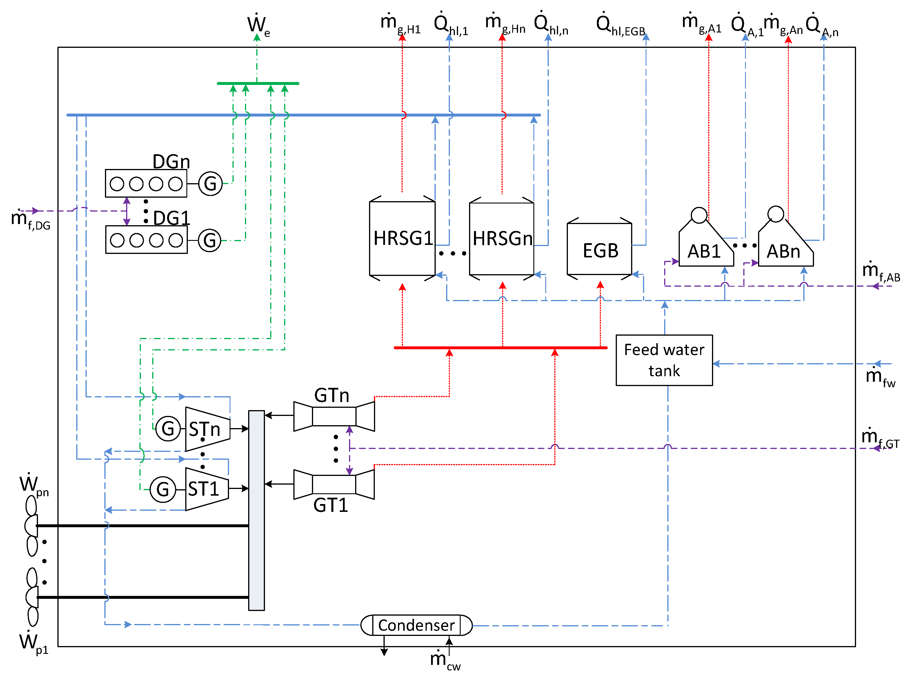
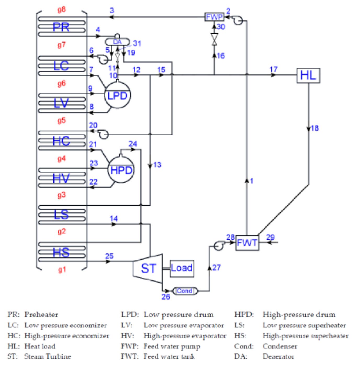
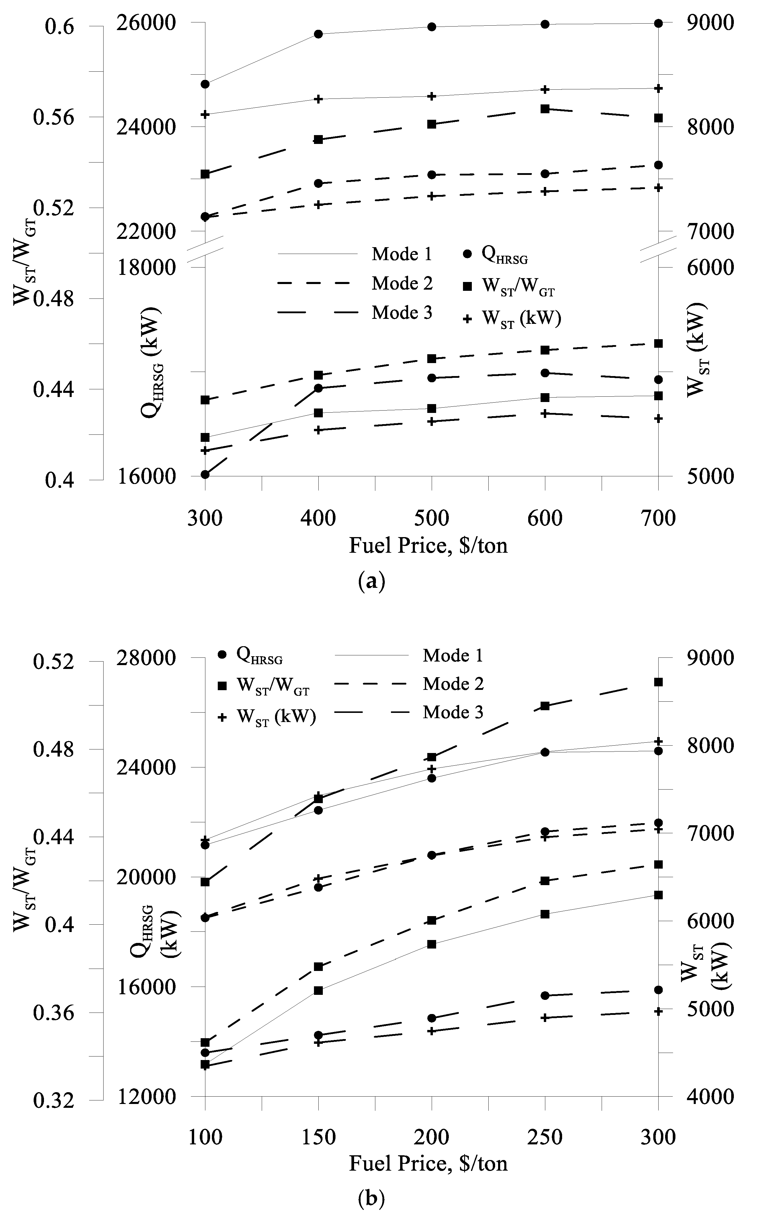
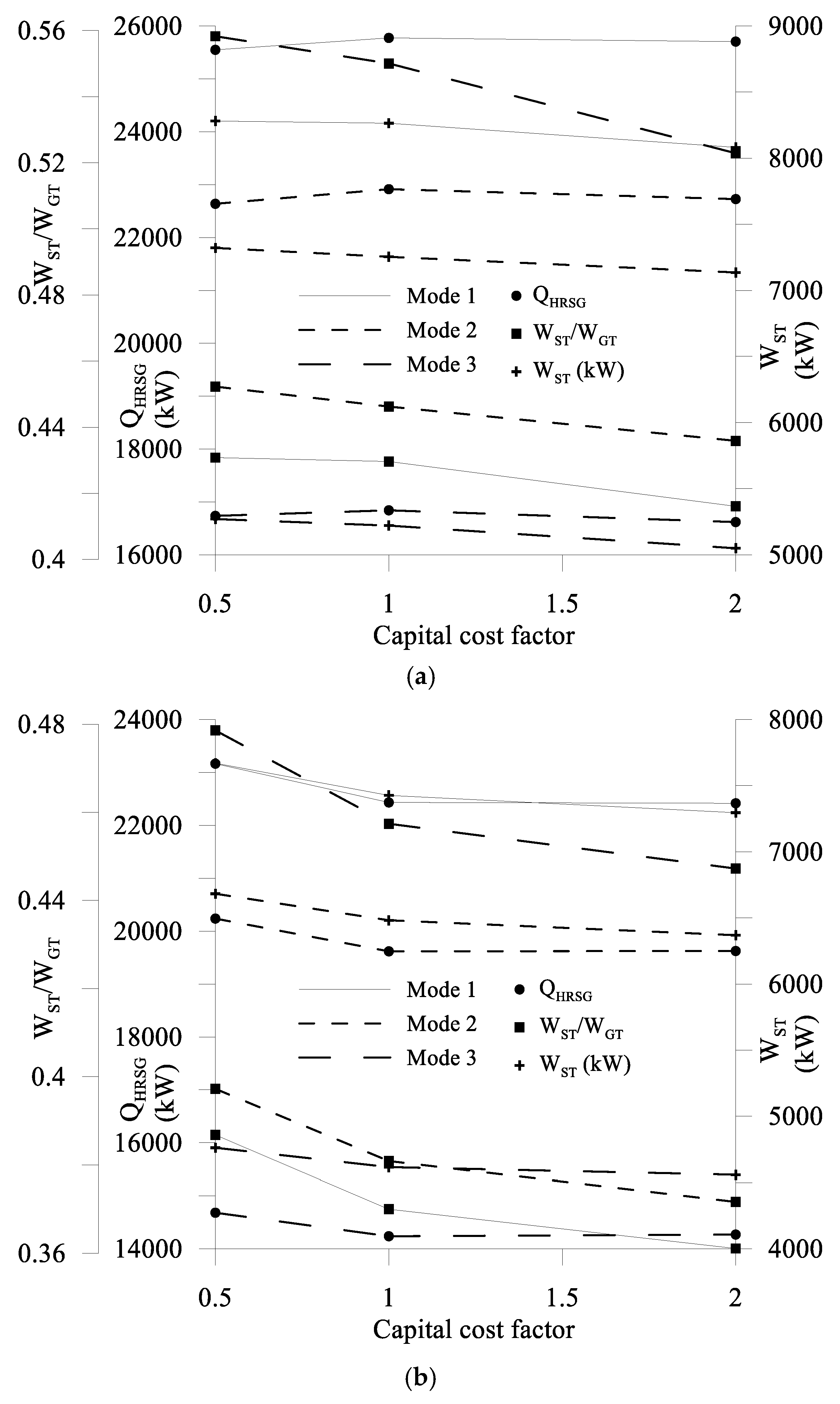
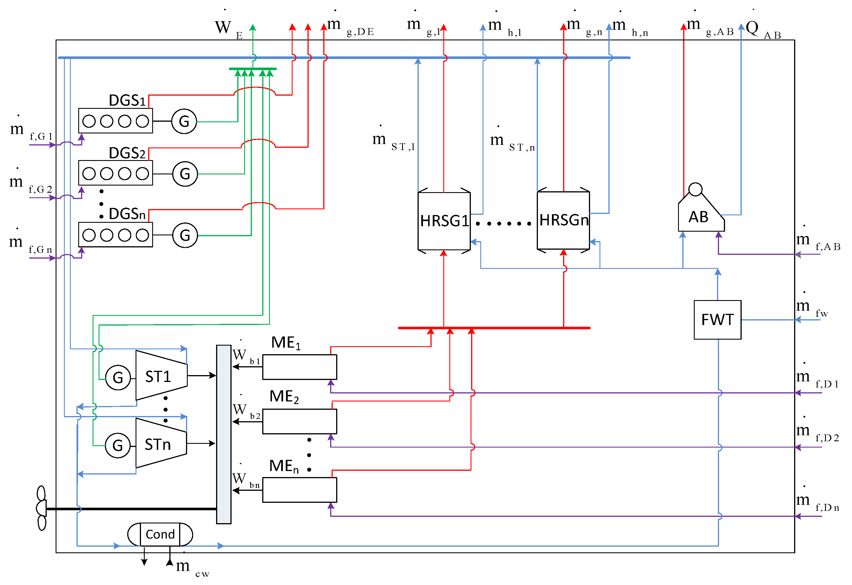
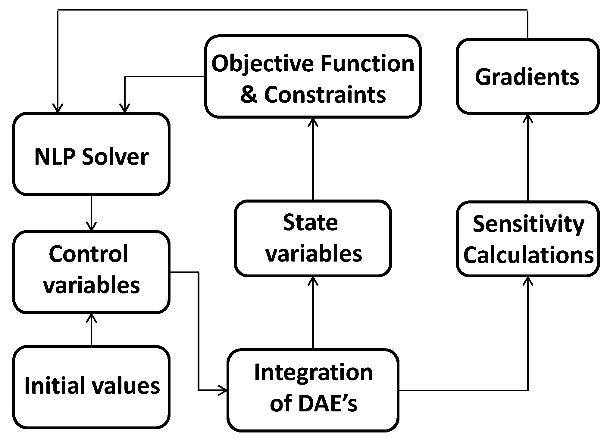
Table A1.
Coefficients for Equation (A1).
| Coefficient | GT Type (a) | GT Type (b) | GT Type (c) |
|---|---|---|---|
| a | 0.451124718450259 | 0.451124718937363 | 0.45112471762403 |
| b | 11.6601660998132 | 11.8085861004949 | 11.9225303717006 |
| c | 8.15305188415185 × 10⁻⁷ | 8.15305206333862 × 10⁻⁷ | 8.15305153736658 × 10⁻⁷ |
The capital costs of other components of the system are estimated as explained in Sakalis and Frangopoulos [24].
Appendix B
Wind speed and direction data for the numerical example of Section 3.
Table A2.
Wind speed (in kn) as a function of time and space in Summer.
| Time (Days) | Distance from Port A (nm) | |||||
|---|---|---|---|---|---|---|
| 513 | 1026 | 1539 | 2052 | 2565 | 3078 | |
| 1 | 4.43 | 4.91 | 4.32 | 5.45 | 4.91 | 6.05 |
| 2 | 13.61 | 15.87 | 16.41 | 13.71 | 13.12 | 16.36 |
| 3 | 17.87 | 16.25 | 17.44 | 18.03 | 16.79 | 15.71 |
| 4 | 9.18 | 11.39 | 9.40 | 9.94 | 10.48 | 17.87 |
| 5 | 24.95 | 19.22 | 16.79 | 24.19 | 26.30 | 24.35 |
| 6 | 21.65 | 23.00 | 24.62 | 26.84 | 26.35 | 22.89 |
| 7 | 22.73 | 21.06 | 27.21 | 24.62 | 26.89 | 23.98 |
| 8 | 23.65 | 23.97 | 22.08 | 22.30 | 22.89 | 25.11 |
Table A3.
Wind speed (in kn) as a function of time and space in Fall.
| Time (Days) | Distance from Port A (nm) | |||||
|---|---|---|---|---|---|---|
| 513 | 1026 | 1539 | 2052 | 2565 | 3078 | |
| 1 | 4.75 | 5.35 | 4.75 | 5.94 | 5.35 | 6.53 |
| 2 | 14.85 | 17.22 | 17.82 | 14.85 | 14.25 | 17.82 |
| 3 | 19.60 | 17.82 | 19.01 | 19.60 | 18.41 | 17.22 |
| 4 | 10.10 | 12.47 | 10.10 | 10.69 | 11.28 | 19.60 |
| 5 | 27.32 | 20.79 | 18.41 | 26.13 | 28.51 | 27.73 |
| 6 | 23.76 | 24.95 | 26.73 | 29.10 | 28.51 | 26.95 |
| 7 | 24.95 | 23.16 | 29.70 | 26.73 | 29.10 | 23.76 |
| 8 | 25.54 | 26.13 | 23.76 | 24.35 | 24.95 | 24.95 |
Table A4.
Wind speed (in kn) as a function of time and space in Winter.
| Time (Days) | Distance from Port A (nm) | |||||
|---|---|---|---|---|---|---|
| 513 | 1026 | 1539 | 2052 | 2565 | 3078 | |
| 1 | 5.23 | 5.88 | 5.23 | 6.53 | 5.88 | 7.19 |
| 2 | 16.33 | 18.95 | 19.60 | 16.33 | 15.68 | 19.60 |
| 3 | 21.56 | 19.60 | 20.91 | 21.56 | 20.25 | 18.95 |
| 4 | 11.11 | 13.72 | 11.11 | 11.76 | 12.41 | 21.56 |
| 5 | 30.05 | 22.87 | 20.25 | 28.75 | 31.36 | 29.40 |
| 6 | 26.13 | 27.44 | 29.40 | 32.01 | 31.36 | 28.44 |
| 7 | 27.44 | 25.48 | 32.67 | 29.40 | 32.01 | 28.13 |
| 8 | 28.09 | 28.75 | 26.13 | 26.79 | 28.44 | 29.44 |
Table A5.
Wind speed (in kn) as a function of time and space in Spring.
| Time (Days) | Distance from Port A (nm) | |||||
|---|---|---|---|---|---|---|
| 513 | 1026 | 1539 | 2052 | 2565 | 3078 | |
| 1 | 3.89 | 4.37 | 3.89 | 4.86 | 4.37 | 5.35 |
| 2 | 12.15 | 14.09 | 14.58 | 12.15 | 11.66 | 14.58 |
| 3 | 16.04 | 14.58 | 15.55 | 16.04 | 15.06 | 14.09 |
| 4 | 8.26 | 10.21 | 8.26 | 8.75 | 9.23 | 16.04 |
| 5 | 22.35 | 17.01 | 15.06 | 21.38 | 23.33 | 21.87 |
| 6 | 19.44 | 20.41 | 21.87 | 23.81 | 23.33 | 20.41 |
| 7 | 20.41 | 18.95 | 24.30 | 21.87 | 23.81 | 19.94 |
| 8 | 20.90 | 21.38 | 19.44 | 19.92 | 22.41 | 21.41 |
Table A6.
Wind direction in degrees (°) with respect to north, counting counterclockwise, as a function of time and space for all seasons.
Table A6.
Wind direction in degrees (°) with respect to north, counting counterclockwise, as a function of time and space for all seasons.
| Time (Days) | Distance from Port A (nm) | |||||
|---|---|---|---|---|---|---|
| 513 | 1026 | 1539 | 2052 | 2565 | 3078 | |
| 1 | 318 | 320 | 310 | 345 | 300 | 260 |
| 2 | 315 | 330 | 330 | 330 | 300 | 250 |
| 3 | 315 | 325 | 334 | 300 | 285 | 260 |
| 4 | 320 | 325 | 330 | 250 | 265 | 255 |
| 5 | 321 | 328 | 345 | 260 | 244 | 230 |
| 6 | 317 | 320 | 305 | 255 | 230 | 225 |
| 7 | 323 | 333 | 300 | 245 | 250 | 228 |
| 8 | 320 | 330 | 328 | 260 | 242 | 230 |
References
- Frangopoulos, C.A. Recent developments and trends in optimization of energy systems. Energy 2018, 164, 1011–1020. [Google Scholar] [CrossRef]
- Frangopoulos, C.A.; Von Spakovsky, M.R.; Sciubba, E.A. Brief Review of Methods for the Design and Synthesis Optimization of Energy Systems. Int. J. Appl. Thermodyn. 2002, 5, 151–160. [Google Scholar]
- Pelster, S.; Favrat, D.; Von Spakovsky, M.R. The Thermoeconomic and Environomic Modeling and Optimization of the Synthesis, Design, and Operation of Combined Cycles with Advanced Options. J. Eng. Gas Turbines Power 2001, 123, 717–726. [Google Scholar] [CrossRef]
- Mussati, S.F.; Aguirre, P.A.; Scenna, N.J. A Rigorous, Mixed-integer, Nonlineal Programming Model (MINLP) for Synthesis and Optimal Operation of Cogeneration Seawater Desalination Plants. Desalination 2004, 166, 339–345. [Google Scholar] [CrossRef]
- Sun, L.; Gai, L.; Smith, R. Site Utility System Optimization with Operation Adjustment under Uncertainty. Appl. Energy 2017, 186, 450–456. [Google Scholar]
- Calise, F.; Dentice d’ Accadia, M.; Vanoli, L.; Von Spakovsky, M.R. Full Load Synthesis/Design Optimization of a Hybrid SOFC–GT Power Plant. Energy 2007, 32, 446–458. [Google Scholar] [CrossRef]
- Toffolo, A. A Synthesis/Design Optimization Algorithm for Rankine Cycle Based Energy Systems. Energy 2014, 66, 115–127. [Google Scholar] [CrossRef]
- Frangopoulos, C.A. Intelligent Functional Approach: A Method for Analysis and Optimal Synthesis–Design–Operation of Complex Systems. Int. J. Energy Environ. Econ. 1991, 1, 267–274. [Google Scholar]
- Frangopoulos, C.A. Optimization of Synthesis–Design–Operation of a Cogeneration System by the Intelligent Functional Approach. Int. J. Energy Environ. Econ. 1991, 1, 275–287. [Google Scholar]
- Frangopoulos, C.A. Optimal Synthesis and Operation of Thermal Systems by the Thermoeconomic Functional Approach. J. Eng. Gas Turbines Power 1992, 114, 707–714. [Google Scholar] [CrossRef]
- Munoz, J.R.; Von Spakovsky, M.R. A Decomposition Approach for the Large Scale Synthesis/Design Optimization of Highly Coupled, Highly Dynamic Energy Systems. Int. J. Appl. Thermodyn. 2001, 4, 19–33. [Google Scholar]
- Munoz, J.R.; Von Spakovsky, M.R. The Application of Decomposition to the Large Scale Synthesis/Design Optimization of Aircraft Energy Systems. Int. J. Appl. Thermodyn. 2001, 4, 61–76. [Google Scholar]
- Rancruel, D.F.; Von Spakovsky, M.R. Decomposition with Thermoeconomic Isolation Applied to the Optimal Synthesis/Design of an Advanced Tactical Aircraft System. Int. J. Thermodyn. 2003, 6, 93–105. [Google Scholar] [CrossRef]
- Georgopoulos, N.G.; Von Spakovsky, M.R.; Muñoz, J.R. A Decomposition Strategy Based on Thermoeconomic Isolation Applied to the Optimal Synthesis/Design and Operation of a Fuel Cell Based Total Energy System. In Proceedings of the IMECE2002 ASME, International Mechanical Engineering Congress & Exposition, New Orleans, LA, USA, 17–22 November 2002. [Google Scholar]
- Oyarzabal, B.; Von Spakovsky, M.R.; Ellis, M.W. Optimal Synthesis/Design of a PEM Fuel Cell Cogeneration System for Multi-unit Residential Applications–Application of a Decomposition Strategy. J. Energy Resour. Technol. 2004, 126, 30–39. [Google Scholar] [CrossRef]
- Munoz, J.R.; Von Spakovsky, M.R. Decomposition in Energy System Synthesis/Design Optimization for Stationary and Aerospace Applications. J. Aircr. 2003, 40, 35–42. [Google Scholar]
- Olsommer, B.; Favrat, D.; Von Spakovsky, M.R. An Approach for the Time-dependent Thermoeconomic Modeling and Optimization of Energy System Synthesis, Design and Operation Part I: Methodology and Results. Int. J. Appl. Thermodyn. 1999, 2, 97–114. [Google Scholar]
- Lazzaretto, A.; Toffolo, A. A method to separate the problem of heat transfer interactions in the synthesis of thermal systems. Energy 2008, 33, 163–170. [Google Scholar] [CrossRef]
- Toffolo, A.; Lazzaretto, A.; Morandin, M. The HEATSEP method for the synthesis of thermal systems: An application to the S-Graz cycle. Energy 2010, 35, 976–981. [Google Scholar] [CrossRef]
- Lazzaretto, A.; Manente, G.; Toffolo, A. SYNTHSEP: A general methodology for the synthesis of energy system configurations beyond superstructures. Energy 2018, 147, 924–949. [Google Scholar] [CrossRef]
- Dimopoulos, G.G.; Kougioufas, A.V.; Frangopoulos, C.A. Synthesis, Design and Operation Optimization of a Marine Energy System. Energy 2008, 33, 180–188. [Google Scholar] [CrossRef]
- Dimopoulos, G.G.; Frangopoulos, C.A. Synthesis, Design and Operation Optimization of the Marine Energy System for a Liquefied Natural Gas Carrier. Int. J. Thermodyn. 2008, 11, 203–211. [Google Scholar]
- Kalikatzarakis, M.; Frangopoulos, C.A. Thermo-economic Optimization of Synthesis, Design and Operation of a Marine Organic Rankine Cycle System. Proc Inst. Mech. Eng. Part M J. Eng. Marit. Environ. 2017, 231, 137–152. [Google Scholar] [CrossRef]
- Sakalis, G.N.; Frangopoulos, C.A. Intertemporal optimization of synthesis, design and operation of integrated energy systems of ships: General method and application on a system with Diesel main engines. Appl. Energy 2018, 226, 991–1008. [Google Scholar] [CrossRef]
- Rancruel, D.F. Dynamic Synthesis/Design and Operational/Control Optimization Approach Applied to a Solid Oxide Fuel Cell Based Auxiliary Power Unit Under Transient Conditions. Ph.D. Dissertation, Virginia Polytechnic Institute and State University, Blacksburg, VA, USA, 2005. [Google Scholar]
- Rancruel, D.F.; Von Spakovsky, M.R. Development and Application of a Dynamic Decomposition Strategy for the Optimal Synthesis/Design and Operational/Control of a SOFC Based APU under Transient Conditions. In Proceedings of the International Mechanical Engineering Congress and Exposition—IMECE, Orlando, FL, USA, 5–11 November 2005; ASME: New York, NY, USA, 2005. Paper No. 82986. [Google Scholar]
- Wang, M.; Kim, K.; Von Spakovsky, M.R.; Nelson, D. Multi- versus Single-level of Dynamic Synthesis/Design and Operation/Control Optimizations of a PEMFC System. In Proceeding of the IMECE2008—ASME International Mechanical Engineering Congress and Exposition, Boston, MA, USA, 31 October–6 November 2008. [Google Scholar]
- Kim, K.; Von Spakovsky, M.R.; Wang, M.; Nelson, D.J. A Hybrid Multi-level Optimization Approach for the Dynamic Synthesis/Design and Operation/Control under Uncertainty of a Fuel Cell System. Energy 2011, 36, 3933–3943. [Google Scholar] [CrossRef]
- Kim, K.; Wang, M.; Von Spakovsky, M.R.; Nelson, D.J. Dynamic Synthesis/Design and Operation/Control Optimization under Uncertainty of a PEMFC System. In Proceedings of the IMECE 2008 ASME International Mechanical Engineering Congress and Exposition, Boston, MA, USA, 31 October–6 November 2008; ASME: New York, NY, USA, 2008. paper no. 68070. pp. 679–689. [Google Scholar]
- Arcuri, P.; Beraldi, P.; Florio, F.; Fragiacomo, P. Optimal Design of a Small Size Trigeneration Plant in Civil Users: A MINLP (Mixed Integer Non Linear Programming) Model. Energy 2015, 80, 628–641. [Google Scholar] [CrossRef]
- Buoro, D.; Casisi, M.; Pinamonti, P.; Reini, M. Optimal Synthesis and Operation of Advanced Energy Supply Systems for Standard and Domotic Home. Energy Convers. Manag. 2012, 60, 96–105. [Google Scholar] [CrossRef]
- Petruschke, P.; Gasparovic, G.; Voll, P.; Krajacic, G.; Duic, N.; Bardow, A. A Hybrid Approach for the Efficient Synthesis of Renewable Energy Systems. Appl. Energy 2014, 135, 625–633. [Google Scholar] [CrossRef]
- Goderbauer, S.; Bahl, B.; Voll, P.; Lübbeckeb, M.; Bardow, A.; Koster, A.M.C.A. An Adaptive Discretization MINLP Algorithm for Optimal Synthesis of Decentralized Energy Supply Systems. Comput. Chem. Eng. 2016, 95, 38–48. [Google Scholar] [CrossRef]
- Zhu, Q.; Luo, X.; Zhang, B.; Chen, Y. Mathematical Modeling and Optimization of a Large–scale Combined Cooling, Heat and Power System that Incorporates Unit Changeover and Time–of–use Electricity Price. Energy Convers. Manag. 2017, 133, 385–398. [Google Scholar]
- Fuentes–Cortés, L.F.; Ponce–Ortega, J.M.; Nápoles–Rivera, F.; Serna–González, M.; El–Halwagi, M. Optimal Design of Integrated CHP Systems for Housing Complexes. Energy Convers. Manag. 2015, 99, 252–263. [Google Scholar] [CrossRef]
- Hanglid, F. A review on the use of gas and steam turbine combined cycles as prime movers for large ships. Part I: Background and design. Energy Convers. Manag. 2008, 49, 3458–3467. [Google Scholar]
- Hanglid, F. A review on the use of gas and steam turbine combined cycles as prime movers for large ships. Part II: Previous work and implications. Energy Convers. Manag. 2008, 49, 3468–3475. [Google Scholar]
- Hanglid, F. A review on the use of gas and steam turbine combined cycles as prime movers for large ships. Part III: Fuels and emissions. Energy Convers. Manag. 2008, 49, 3476–3482. [Google Scholar]
- Altosole, M.; Benvenuto, G.; Campora, U.; Laviola, M.; Trucco, A. Waste Heat Recovery from Marine Gas Turbines and Diesel Engines. Energies 2017, 10, 718. [Google Scholar] [CrossRef]
- Dzida, M. Comparing combined gas tubrine/steam turbine and marine low speed piston engine/steam turbine systems in naval applications. Pol. Marit. Res. 2011, 18, 43–48. [Google Scholar] [CrossRef] [Green Version]
- Hanglid, F. Variable geometry gas turbines for improving the part–load performance of marine combined cycles—Gas turbine performance. Energy 2010, 35, 562–570. [Google Scholar]
- Hanglid, F. Variable geometry gas turbines for improving the part–load performance of marine combined cycles—Combined cycle performance. Appl. Therm. Eng. 2011, 31, 467–476. [Google Scholar]
- Wang, Z.; Li, J.; Fan, K.; Li, S. The Off–Design Performance Simulation of Marine Gas Turbine Based on Optimum Scheduling of Variable Stator Vanes. Math. Probl. Eng. 2017, 2671251. [Google Scholar] [CrossRef]
- Sharma, O.P.; Kaushik, S.C.; Manjunath, K. Thermodynamic analysis and optimization of a supercritical CO2 regenerative recompression Brayton cycle coupled with a marine gas turbine for shipboard waste heat recovery. Therm. Sci. Eng. Prog. 2017, 3, 62–74. [Google Scholar] [CrossRef]
- Hou, S.; Wu, Y.; Zhou, Y.; Yu, L. Performance analysis of the combined supercritical CO2 recompression and regenerative cycle used in waste heat recovery of marine gas turbine. Energy Convers. Manag. 2017, 151, 73–85. [Google Scholar] [CrossRef]
- Wang, Z.; Li, Y.G.; Li, S. Performance simulation of 3–stage gas turbine CHP plant for marine applications. In Proceedings of the ASME Turbo Expo 2016: Turbomachinery Technical Conference and Exposition GT2016, Seoul, Korea, 13–17 June 2016. GT2016–56312. [Google Scholar]
- Welaya, Y.M.A.; Mosleh, M.; Ammar, N.R. Thermodynamic analysis of a combined gas turbine power plant with a solid oxide fuel cell for marine applications. Int. J. Nav. Archit. Ocean Eng. 2013, 5, 529–545. [Google Scholar] [CrossRef] [Green Version]
- Tse, L.K.C.; Wilkins, S.; McGlashana, N.; Urbanb, B.; Martinez–Botasa, R. Solid oxide fuel cell/gas turbine trigeneration system for marine applications. J. Power Sources 2011, 196, 3149–3162. [Google Scholar] [CrossRef]
- Armellini, A.; Daniotti, S.; Pinamonti, P. Gas Turbines for power generation on board of cruise ships: A possible solution to meet the new IMO regulations? Energy Procedia 2015, 81, 540–547. [Google Scholar] [CrossRef]
- Armellini, A.; Daniotti, S.; Pinamonti, P.; Reini, M. Evaluation of gas turbines as alternative energy production systems for a large cruise ship to meet new maritime regulations. Appl. Energy 2018, 211, 306–317. [Google Scholar] [CrossRef]
- Doulgeris, G.; Korakianitis, T.; Pilidis, P.; Tsoudis, E. Techno–economic and environmental risk analysis for advanced marine propulsion systems. Appl. Energy 2012, 99, 1–12. [Google Scholar] [CrossRef]
- De Leon, L.S.; Zachos, P.K.; Pachidis, V. A comparative assessment of dry gas turbine cycles for marine applications. In Proceedings of the ASME Turbo Expo 2013: Turbine Technical Conference and Exposition GT2013, San Antonio, TX, USA, 3–7 June 2013. GT2013–95321. [Google Scholar]
- Ji, N.; Li, S.; Wang, Z.; Zhao, N. Off–Design Behavior Analysis and Operating Curve Design of Marine Intercooled Gas Turbine. Math. Probl. Eng. 2017, 8325040. [Google Scholar] [CrossRef]
- El-Gohary, M.M.; Seddiek, I.S. Utilization of alternative marine fuels for gas turbine power plant onboard ships. Int. J. Nav. Arch. Ocean Eng. 2013, 5, 21–32. [Google Scholar] [CrossRef] [Green Version]
- El-Gohary, M.M.; Ammar, N.R. Thermodynamic analysis of alternative marine fuels for marine gas turbine power plants. J. Mar. Sci. Appl. 2016, 15, 95–103. [Google Scholar] [CrossRef]
- El-Gohary, M.M. The future of natural gas as a fuel in marine gas turbine for LNG carriers. Proc. Inst. Mech. Eng. Part M J. Eng. Marit. Environ. 2012, 226, 371–377. [Google Scholar] [CrossRef]
- Fernández, I.A.; Gómez, M.R.; Gómez, J.R.; Insuab, Á.B. Review of propulsion systems on LNG carriers. Renew. Sustain. Energy Rev. 2017, 67, 1395–1411. [Google Scholar] [CrossRef]
- Software MarineGTs, Laboratory of Thermal Turbomachines, National Technical University of Athens, Greece. Information. Available online: https://www.ltt.ntua.gr/index.php/en/softwaremn/marine-gts (accessed on 2 January 2019).
- Frangopoulos, C.A. Application of the thermoeconomic functional approach to the CGAM problem. Energy 1994, 19, 323–342. [Google Scholar] [CrossRef]
- Tzortzis, G.J.; Frangopoulos, C.A. Dynamic optimization of synthesis, design and operation of marine energy systems. J. Eng. Marit. Environ. 2018. [Google Scholar] [CrossRef]
- gPROMS. User Guide, version 4.1.1; Process Systems Enterprise Ltd.: London, UK, 2016.
- Bard, Y. Nonlinear Parameter Estimation; Academic Press: New York, NY, USA, 1974. [Google Scholar]
- Internet Sites with Weather Data. Available online: https://earth.nullschool.net and http://www.meteoearth.com and http://www.accuweather.com and http://enterprisesolutions.accuweather.com (accessed on 15 July 2017).
Figure 1.
The three interrelated levels of optimization.

Figure 2.
Superconfiguration of the energy system.

Figure 3.
The three gas turbine types considered as main engines.

Figure 4.
Bottoming cycle and internal structure of the HRSG.

Figure 5.
Variation of specific fuel consumption (SFC) and exhaust gas characteristics in partial load operation (fuel MDO).
Figure 5.
Variation of specific fuel consumption (SFC) and exhaust gas characteristics in partial load operation (fuel MDO).

Figure 6.
(a) Effect of MDO price on the optimal values of , and (b) the effect of natural gas price on the optimal values of , , and .
Figure 6.
(a) Effect of MDO price on the optimal values of , and (b) the effect of natural gas price on the optimal values of , , and .

Figure 7.
(a) Effect of capital cost on the optimal values of and and on the fraction with MDO. (b) Effect of capital cost on the optimal values of and and on the fraction for natural gas.
Figure 7.
(a) Effect of capital cost on the optimal values of and and on the fraction with MDO. (b) Effect of capital cost on the optimal values of and and on the fraction for natural gas.

Figure 8.
Superconfiguration of the generic energy system. (AB: auxiliary boiler; Cond: condenser; DGS: Diesel generator set; FWT: feed water tank, G: generator; HRSG: heat recovery steam generator; ME: main engine, ST: steam turbine).
Figure 8.
Superconfiguration of the generic energy system. (AB: auxiliary boiler; Cond: condenser; DGS: Diesel generator set; FWT: feed water tank, G: generator; HRSG: heat recovery steam generator; ME: main engine, ST: steam turbine).

Figure 9.
Sketch of the sequential approach used.

Table 1.
Independent variables of the optimization problem.
Table 2.
Natural gas composition.
| Component | Composition % Volume |
|---|---|
| CH4 | 88.5 |
| C2H6 | 4.7 |
| C3H8 | 1.6 |
| C4H10 | 0.2 |
| N2 | 5.0 |
Table 3.
Annual energy profile of the ship.
| Mode y | ||||
|---|---|---|---|---|
| 1 | 26,000 | 1500 | 400 | 2690 |
| 2 | 22,000 | 1500 | 300 | 1575 |
| 3 | 14,000 | 700 | 200 | 1620 |
| 4 | 0 | 1200 | 150 | 1000 |
Table 4.
Values of economic parameters.
| Parameter | Value | Parameter | Value |
|---|---|---|---|
| cf,MDO | 400$/ton | com,GT | 0.006$/kWh |
| cf,NG | 150$/ton | com,DG | 0.007$/kWh |
| NY | 20 | com,HRSG , com,AB | 0.005$/kWh |
| f | 3% | com,ST | 0.004$/kWh |
| i | 8% | com,GT | 0.006$/kWh |
Table 5.
Optimal synthesis of the system.
| |
Table 6.
Optimal design characteristics and capital cost of components for the six combinations of gas turbine type and fuel.
Table 6.
Optimal design characteristics and capital cost of components for the six combinations of gas turbine type and fuel.
| Type/Fuel | (a)/MDO | (b)/MDO | (c)/MDO | (a)/NG | (b)/NG | (c)/NG |
|---|---|---|---|---|---|---|
| 23828 | 26941 | 28656 | 24662 | 27373 | 29379 | |
| 23663 | 19708 | 13765 | 20623 | 15799 | 9605 | |
| 47.36 | 77.57 | 62.27 | 54.42 | 67.48 | 54.47 | |
| 5.561 | 4.532 | 3.091 | 5.565 | 3.904 | 2.663 | |
| 1.631 | 2.136 | 1.604 | 0.608 | 1.263 | 0.442 | |
| 63.58 | 17.65 | 19.23 | 63.67 | 21.66 | 23.29 | |
| 6.12 | 4.71 | 4.27 | 9.00 | 7.71 | 7.25 | |
| 584.90 | 377.12 | 348.63 | 554.08 | 420.34 | 387.15 | |
| 153.57 | 157.77 | 157.8 | 226.91 | 218.22 | 234.92 | |
| 552.46 | 347.26 | 316.43 | 522.89 | 387.34 | 354.53 | |
| 182.85 | 170.55 | 174.51 | 199.51 | 187.29 | 188.97 | |
| 8624 | 5009 | 3376 | 7589 | 4925 | 2706 | |
| 6.431 | 4.696 | 3.139 | 6.276 | 4.505 | 2.944 | |
| 1.608 | 2.111 | 1.590 | 0.549 | 1.320 | 0.458 | |
| 543.53 | 327.49 | 307.88 | 513.43 | 386.07 | 324.17 | |
| 179.87 | 162.31 | 171.1 | 187.96 | 207.95 | 193.76 | |
| 1206 | 1210 | 1203 | 1207 | 1209 | 1207 | |
| 10,718,229 | 13,107,957 | 15,083,626 | 10,878,489 | 13,197,730 | 15,245,075 | |
| 2,684,082 | 2,344,735 | 1,905,809 | 2,332,648 | 1,621,354 | 1,110,526 | |
| 1,498,472 | 1,202,482 | 993,061 | 1,425,071 | 1,151,211 | 887,139 | |
| 874,689 | 875,808 | 873,849 | 874,958 | 875,529 | 874,969 |
Table 7.
Operational technical and economic characteristics for the system with gas turbine type (a) and fuel MDO.
Table 7.
Operational technical and economic characteristics for the system with gas turbine type (a) and fuel MDO.
| Mode 1 | Mode 2 | Mode 3 |
|---|---|---|
| 19,240.01 | 16,256.68 | 9491.33 |
| 223.808 | 233.3587 | 275.5277 |
| 25,774.74 | 22,915.2 | 16,841.91 |
| 54.59 | 50.52 | 39.2 |
| 543.07/135.48 | 530.50/138.90 | 510.07/139.16 |
| 6.329 | 5.635 | 4.186 |
| 1.632 | 1.515 | 1.129 |
| 0.1545 | 0.1159 | 0.0772 |
| 8265.38 | 7274.15 | 5226.8 |
| 156.5536 | 161.2199 | 177.6805 |
| GT annual fuel cost ($) | ||
| 463,3329.06 | 2,389,991.03 | 1,694,600.04 |
| GT annual O&M cost ($) | ||
| 310,533.75 | 153,625.61 | 92,255.71 |
| HRSG O&M cost ($) | ||
| 350,171.93 | 182,279.96 | 137,797.45 |
| Steam turbine O&M cost $ | ||
| 88,935.51 | 46,041.35 | 33,999.27 |
Table 8.
Operational technical and economic characteristics for the system with gas turbine type (b) and fuel MDO.
Table 8.
Operational technical and economic characteristics for the system with gas turbine type (b) and fuel MDO.
| Mode 1 | Mode 2 | Mode 3 |
|---|---|---|
| 22,324.94 | 18,887.21 | 11,776.75 |
| 199.9417 | 206.3503 | 229.9452 |
| 21,188.97 | 18,445.27 | 12,476.87 |
| 78.21 | 73.76 | 62.69 |
| 378.40/144.49 | 359.51/143.62 | 314.96/143.13 |
| 5.05 | 4.381 | 2.972 |
| 2.12 | 1.928 | 1.379 |
| 0.1552 | 0.1164 | 0.0776 |
| 5175.14 | 4643.9 | 2938.45 |
| 162.3154 | 165.6268 | 184.0279 |
| GT annual fuel cost ($) | ||
| 4,802,925.31 | 2,455,350.95 | 1,754,787.9 |
| GT annual O&M cost ($) | ||
| 360,324.5 | 178,484.18 | 114,469.96 |
| HRSG annual O&M cost ($) | ||
| 287,870.41 | 146,723.72 | 102,083.46 |
| Steam turbine annual O&M cost ($) | ||
| 55,684.52 | 29,256.6 | 19,365.14 |
Table 9.
Operational technical and economic characteristics for the system with gas turbine type (c) and fuel MDO.
Table 9.
Operational technical and economic characteristics for the system with gas turbine type (c) and fuel MDO.
| Mode 1 | Mode 2 | Mode 3 |
|---|---|---|
| 24,058.85 | 20,517.82 | 12,884.59 |
| 185.0074 | 189.1652 | 204.3804 |
| 14,274.47 | 12,308.24 | 8190.35 |
| 58.99 | 54.96 | 44.28 |
| 356.47/147.56 | 340.05/146.72 | 307.06/147.37 |
| 3.304 | 2.81 | 1.84 |
| 1.557 | 1.427 | 1.017 |
| 0.1554 | 0.1166 | 0.0777 |
| 3444.36 | 2997.19 | 1833.82 |
| 161.8380 | 165.0545 | 178.9159 |
| GT annual fuel cost ($) | ||
| 4,789,345.29 | 2,445,191.84 | 1,706,415.29 |
| GT annual O&M cost ($) | ||
| 388,309.76 | 193,893.47 | 125,238.22 |
| HRSG annual O&M cost ($) | ||
| 193,930.97 | 97,906.42 | 67,011.93 |
| Steam turbine O&M cost ($) | ||
| 37,061.28 | 18,882.29 | 12,207.16 |
Table 10.
Operational technical and economic characteristics for the system with gas turbine type (a) and fuel NG.
Table 10.
Operational technical and economic characteristics for the system with gas turbine type (a) and fuel NG.
| Mode 1 | Mode 2 | Mode 3 |
|---|---|---|
| 20,074.11 | 17,020.17 | 10,089.86 |
| 206.1992 | 213.9852 | 248.7073 |
| 22,434.93 | 19,618.54 | 14,238.04 |
| 55.03 | 51.31 | 40.34 |
| 541.77/189.81 | 525.31/195.20 | 500.82/196.08 |
| 6.186 | 5.472 | 4.037 |
| 0.592 | 0.521 | 0.374 |
| 0.1535 | 0.1151 | 0.0768 |
| 7427.69 | 6482.47 | 4615.36 |
| 150.5089 | 154.9641 | 170.6484 |
| GT annual fuel cost ($) | ||
| 1,670,193.45 | 860,437.60 | 609,789.37 |
| GT annual O&M cost ($) | ||
| 323,996.13 | 160,840.64 | 98,073.42 |
| HRSG annual O&M cost ($) | ||
| 304,797.79 | 156,056.61 | 116,493.10 |
| Steam turbine O&M cost ($) | ||
| 79,921.97 | 40,839.54 | 29,907.51 |
Table 11.
Operational technical and economic characteristics for the system with gas turbine type (b) and fuel NG.
Table 11.
Operational technical and economic characteristics for the system with gas turbine type (b) and fuel NG.
| Mode 1 | Mode 2 | Mode 3 |
|---|---|---|
| 22,785.05 | 19,424.37 | 12,170.46 |
| 185.0029 | 190.456 | 211.1788 |
| 17,376.5 | 15,159.49 | 9817.69 |
| 77.38 | 73.12 | 62.1 |
| 382.16/188.30 | 363.97/184.99 | 319.25/182.76 |
| 4.449 | 3.921 | 2.56 |
| 1.349 | 1.196 | 0.828 |
| 0.1539 | 0.1154 | 0.0769 |
| 4716.93 | 4092.76 | 2532.37 |
| 154.2726 | 157.3103 | 174.8060 |
| GT annual fuel cost ($) | ||
| 1,700,873.65 | 874,003.99 | 624,544.51 |
| GT annual O&M cost ($) | ||
| 367,750.71 | 183,560.28 | 118,296.86 |
| HRSG annual O&M cost ($) | ||
| 236,074.62 | 120,586.84 | 80,326.59 |
| Steam turbine annual O&M cost ($) | ||
| 50,754.12 | 25,784.36 | 16,409.77 |
Table 12.
Operational technical and economic characteristics for the system with gas turbine type (c) and fuel NG.
Table 12.
Operational technical and economic characteristics for the system with gas turbine type (c) and fuel NG.
| Mode 1 | Mode 2 | Mode 3 |
|---|---|---|
| 24,790.93 | 21,155.23 | 132,36.94 |
| 171.9147 | 175.8823 | 190.2175 |
| 10,311.13 | 8965.8 | 5865.57 |
| 59.51 | 55.89 | 45.2 |
| 360.39/210.81 | 342.95/204.46 | 308.26/196.24 |
| 2.934 | 2.584 | 1.706 |
| 0.459 | 0.409 | 0.286 |
| 0.154 | 0.1155 | 0.077 |
| 2709.48 | 2348.92 | 1471.93 |
| 153.9768 | 158.3053 | 171.1823 |
| GT annual fuel cost ($) | ||
| 1,719,687.12 | 879,046.09 | 611,849.37 |
| GT annual O&M cost ($) | ||
| 400,125.68 | 199,916.93 | 128,663.12 |
| HRSG annual O&M cost ($) | ||
| 140,085.56 | 71,318.87 | 47,991.06 |
| Steam turbine annual O&M cost ($) | ||
| 29,154.02 | 14,798.17 | 9538.08 |
Table 13.
Optimal PWC for the six combinations of gas turbines and fuels.
| Type of Gas Turbine | PWC | |
|---|---|---|
| MDO | NG | |
| A | 141,171,375 | 71,545,007 |
| B | 145,300,524 | 72,237,706 |
| C | 143,784,701 | 71,711,376 |
Table 14.
Optimal design characteristics and capital cost of the system components for various MDO prices.
Table 14.
Optimal design characteristics and capital cost of the system components for various MDO prices.
| Fuel Price ($/ton) | 300 | 400 | 500 | 600 | 700 |
|---|---|---|---|---|---|
| 23,976 | 23,828 | 23,803 | 23,739 | 23,731 | |
| 22,688 | 23,663 | 24,293 | 25,893 | 26,579 | |
| 47.53 | 47.36 | 48.22 | 51.07 | 51.82 | |
| 5.461 | 5.561 | 5.708 | 6.078 | 6.224 | |
| 1.351 | 1.631 | 1.696 | 1.799 | 1.838 | |
| 65.34 | 63.58 | 66.25 | 66.62 | 65.62 | |
| 8.24 | 6.12 | 5.73 | 5.67 | 5.68 | |
| 592.00 | 584.90 | 585.18 | 585.72 | 590.07 | |
| 179.90 | 153.57 | 150.20 | 148.03 | 147.24 | |
| 560.26 | 552.46 | 550.63 | 555.46 | 561.56 | |
| 193.51 | 182.85 | 180.53 | 179.56 | 176.17 | |
| 8677 | 8624 | 8613 | 8731 | 8636 | |
| 6.380 | 6.431 | 6.412 | 6.396 | 6.384 | |
| 1.320 | 1.608 | 1.658 | 1.670 | 1.730 | |
| 567.72 | 543.53 | 542.84 | 553.76 | 541.26 | |
| 188.78 | 179.87 | 178.17 | 182.69 | 176.23 | |
| 1205 | 1206 | 1204 | 1210 | 1205 | |
| 10,746,899 | 10,718,229 | 10,713,354 | 10,700,901 | 10,699,234 | |
| 2,495,601 | 2,684,082 | 2,777,585 | 2,982,490 | 3,043,967 | |
| 1,485,766 | 1,498,472 | 1,500,705 | 1,506,214 | 1,507,158 | |
| 874,410 | 874,689 | 874,130 | 875,808 | 874,410 |
Table 15.
Optimal design characteristics and capital cost of the system components for various prices of natural gas.
Table 15.
Optimal design characteristics and capital cost of the system components for various prices of natural gas.
| Fuel Price ($/ton) | 100 | 150 | 200 | 250 | 300 |
|---|---|---|---|---|---|
| 25,167 | 24,662 | 24,380 | 24,170 | 23,831 | |
| 19,119 | 20,623 | 22,119 | 23,320 | 23,551 | |
| 57.50 | 54.42 | 50.92 | 50.17 | 47.30 | |
| 5.396 | 5.565 | 5.464 | 5.582 | 5.498 | |
| 0.325 | 0.608 | 1.196 | 1.503 | 1.634 | |
| 62.85 | 63.67 | 65.69 | 65.60 | 67.69 | |
| 7.54 | 9.00 | 9.45 | 7.15 | 6.44 | |
| 538.97 | 554.08 | 575.65 | 575.85 | 591.51 | |
| 251.91 | 226.91 | 200.61 | 174.60 | 161.73 | |
| 507.53 | 522.89 | 544.63 | 544.11 | 559.62 | |
| 191.47 | 199.51 | 199.82 | 189.16 | 185.16 | |
| 6983 | 7589 | 7943 | 8174 | 8491 | |
| 6.254 | 6.276 | 6.152 | 6.231 | 6.329 | |
| 0.290 | 0.549 | 1.096 | 1.386 | 1.531 | |
| 476.26 | 513.43 | 529.52 | 530.73 | 544.12 | |
| 180.24 | 187.96 | 185.65 | 167.34 | 162.92 | |
| 1205 | 1207 | 1208 | 1209 | 1207 | |
| 10,973,925 | 10,878,489 | 10,824,556 | 10,784,367 | 10,718,674 | |
| 2,149,778 | 2,332,648 | 2,454,784 | 2,643,177 | 2,663,628 | |
| 1,378,655 | 1,425,071 | 1,452,170 | 1,469,284 | 1,469,208 | |
| 874,410 | 874,958 | 875,249 | 875,529 | 874,969 |
Table 16.
Optimal PWC for varying fuel price.
| MDO | Natural Gas | ||
|---|---|---|---|
| Fuel Price ($/ton) | PWC ($) | Fuel Price ($/ton) | PWC ($) |
| 300 | 114,302,675 | 100 | 58,889,296 |
| 400 | 141,171,375 | 150 | 71,545,007 |
| 500 | 167,995,232 | 200 | 84,112,723 |
| 600 | 194,661,060 | 250 | 96,522,638 |
| 700 | 221,544,251 | 300 | 110,365,050 |
Table 17.
Optimal design characteristics and capital cost of components for various capital costs.
| Fuel | MDO | Natural Gas | ||||
|---|---|---|---|---|---|---|
| Capital cost factor | 0.5 | 1 | 2 | 0.5 | 1 | 2 |
| 23,811 | 23,828 | 24,014 | 24,420 | 24,662 | 24,793 | |
| 24,659 | 23,663 | 23,489 | 22,124 | 20,623 | 20,427 | |
| 47.05 | 47.36 | 50.84 | 49.36 | 54.42 | 54.84 | |
| 5.720 | 5.561 | 5.437 | 5.652 | 5.565 | 5.560 | |
| 1.716 | 1.631 | 1.762 | 0.890 | 0.608 | 0.506 | |
| 65.52 | 63.58 | 57.47 | 64.09 | 63.67 | 52.50 | |
| 6.72 | 6.12 | 5.06 | 9.12 | 9.00 | 7.44 | |
| 602.23 | 584.90 | 571.27 | 586.45 | 554.08 | 554.76 | |
| 149.76 | 153.57 | 172.40 | 199.45 | 226.91 | 233.17 | |
| 571.52 | 552.46 | 538.83 | 557.20 | 522.89 | 522.39 | |
| 180.02 | 182.85 | 177.36 | 201.83 | 199.51 | 193.40 | |
| 9085 | 8624 | 8323 | 8471 | 7589 | 7491 | |
| 6.264 | 6.431 | 6.386 | 6.281 | 6.276 | 6.296 | |
| 1.701 | 1.608 | 1.625 | 0.879 | 0.549 | 0.494 | |
| 607.69 | 543.53 | 575.96 | 590.38 | 513.43 | 535.96 | |
| 191.89 | 179.87 | 175.92 | 204.76 | 187.96 | 200.54 | |
| 1206 | 1206 | 1209 | 1204 | 1207 | 1209 | |
| 5,357,419 | 10,718,229 | 21,508,254 | 5,416,119 | 10,878,489 | 21,806,551 | |
| 1,398,610 | 2,684,082 | 4,927,116 | 1,251,530 | 2,332,648 | 4,315,563 | |
| 767,846 | 1,498,472 | 2,947,318 | 750,324 | 1,425,071 | 2,832,784 | |
| 437,345 | 874,689 | 1,751,058 | 437,065 | 874,958 | 1,751,058 | |
Table 18.
Optimal PWC and bottoming cycle (BC) costs for varying capital cost factors.
| Fuel | Capital Cost Factor | Total PWC ($) | Capital Cost of BC ($) | PWC of O&M of BC ($) |
|---|---|---|---|---|
| MDO | 0.5 | 132,975,803 | 2,148,514 | 10,310,416 |
| 1 | 141,171,375 | 4,182,555 | 10,280,546 | |
| 2 | 157,641,585 | 7,892,692 | 10,269,102 | |
| NG | 0.5 | 63,561,140 | 1,974,960 | 9,204,124 |
| 1 | 71,545,007 | 3,757,720 | 8,918,232 | |
| 2 | 87,119,816 | 7,141,844 | 8,915,494 |
Table 19.
Vessel dimensions propulsion power and related coefficients for containership.
| Parameter | Symbol | Value |
|---|---|---|
| Ship Dimensions | ||
| Overall length (m) | 336 | |
| Length between perpendiculars (m) | 321 | |
| Length at the waterline (m) | 317 | |
| Breadth (m) | 45 | |
| Draught (m) | 15 | |
| Forward molded draught (m) | 14.7 | |
| Aft molded draught (m) | 15.2 | |
| Draught at midship (m) | 15 | |
| Wetted volume (m2) | 146,491 | |
| Wetted Surface | 19,029 | |
| Ship Hull Coefficients | ||
| Block coefficient | 0.6506 | |
| Prismatic coefficient | 0.6605 | |
| Waterplane area coefficient | 0.8560 | |
| Midship section coefficient | 0.9850 | |
| Longitudinal position at the centre of buoyancy (m) | 152.7 | |
| Height at the centre of transverse area (m) | 22 | |
| Propulsion Power Coefficients | ||
| Bearing efficiency | 0.98 | |
| Stern-tube efficiency | 0.97 | |
| Gearing efficiency | 0.99 | |
| Rotative efficiency | 0.98 | |
| Open water efficiency | 0.99 | |
| Service speed (kn) | 24 | |
| Brake power at service speed (kW) | 69,439 | |
Table 20.
Time schedule of the ship.
| Mode | Description | Duration |
|---|---|---|
| 1 | Off-loading and loading at port A (all seasons) | 2 days |
| 2 | Loaded trip from port A to port B (all seasons) | Variable |
| 3 | Off-loading and loading at port B (all seasons) | 2 days |
| 4 | Loaded trip from port B to port A (all seasons) | Variable |
| Total round trip | Variable |
Table 21.
Thermal power demands for each season.
| Time (Days) | Thermal Power (kW) | |||
|---|---|---|---|---|
| Summer | Fall | Winter | Spring | |
| From port A to port B | ||||
| 1 | 850 | 860 | 1000 | 990 |
| 2 | 880 | 900 | 1050 | 980 |
| 3 | 860 | 950 | 1080 | 1010 |
| 4 | 900 | 970 | 1100 | 1020 |
| 5 | 840 | 930 | 1060 | 950 |
| 6 | 850 | 960 | 1100 | 970 |
| 7 | 845 | 959 | 1100 | 980 |
| 8 | 851 | 963 | 1090 | 970 |
| From port B to port A | ||||
| 1 | 860 | 930 | 1100 | 1040 |
| 2 | 870 | 950 | 1080 | 970 |
| 3 | 870 | 980 | 1060 | 960 |
| 4 | 890 | 970 | 990 | 950 |
| 5 | 860 | 890 | 1040 | 980 |
| 6 | 870 | 910 | 1070 | 960 |
| 7 | 880 | 920 | 1080 | 970 |
| 8 | 870 | 910 | 1050 | 960 |
| Ports | ||||
| A | 950 | 950 | 950 | 950 |
| B | 950 | 950 | 950 | 950 |
Table 22.
Electric power demands for each season.
| Time (Days) | Electric Power (kW) | |||
|---|---|---|---|---|
| Summer | Fall | Winter | Spring | |
| From port A to port B | ||||
| 1 | 1495 | 1508 | 1482 | 1625 |
| 2 | 1599 | 1573 | 1586 | 1599 |
| 3 | 1560 | 1547 | 1482 | 1547 |
| 4 | 1514 | 1560 | 1508 | 1495 |
| 5 | 1508 | 1495 | 1586 | 1534 |
| 6 | 1495 | 1495 | 1495 | 1521 |
| 7 | 1490 | 1495 | 1485 | 1525 |
| 8 | 1495 | 1495 | 1490 | 1520 |
| From port B to port A | ||||
| 1 | 1625 | 1547 | 1534 | 1521 |
| 2 | 1560 | 1625 | 1521 | 1625 |
| 3 | 1534 | 1664 | 1625 | 1573 |
| 4 | 1521 | 1508 | 1651 | 1625 |
| 5 | 1560 | 1501 | 1495 | 1599 |
| 6 | 1521 | 1547 | 1521 | 1586 |
| 7 | 1520 | 1539 | 1520 | 1580 |
| 8 | 1525 | 1550 | 1521 | 1580 |
| Ports | ||||
| A | 1500 | 1500 | 1500 | 1500 |
| B | 1500 | 1500 | 1500 | 1500 |
Table 23.
Economic parameters.
| Parameter | Symbol | Value |
|---|---|---|
| MDO fuel cost nominal value | 0.450 €/kg | |
| HFO fuel cost nominal value | 0.300 €/kg | |
| Technical life of the system | 20 years | |
| Maximum permissible hours of operation—Summer | 2160 | |
| Maximum permissible hours of operation—Fall | 2160 | |
| Maximum permissible hours of operation—Winter | 1450 | |
| Maximum permissible hours of operation—Spring | 2160 | |
| Market interest rate | 10% | |
| Freight rate (nominal value) | 0.0326€/TEU nm | |
| Loading factor of containership | 0.85 |
Table 24.
Bounds on synthesis, design, and operation variables.
| Variable | Lower Value | Upper Value |
|---|---|---|
| Number of gas turbines of (each type) | 0 | 2 |
| Number of 2-X Diesel engines | 0 | 3 |
| Number of 4-X Diesel engines | 0 | 4 |
| Number of total propulsion engines | 1 | 6 |
| Number of DG sets | 0 | 4 |
| Number of HRSGs | 0 | 2 |
| Number of STs | 0 | 2 |
| Gas turbine nominal power output (kW) (any type) | 3000 | 90,000 |
| 2-X Diesel engines nominal power output (kW) | 3500 | 90,000 |
| 4-X Diesel engines nominal power output (kW) | 3500 | 21,000 |
| Generator set nominal power output (kW) | 300 | 5000 |
| Load factors (all equipment) | 0.15 | 1 |
| Ship speed (kn) | 14 | 25.4 |
| Single trip duration (days) | 5 | 8 |
Table 25.
Numerical solution parameters.
| Parameter | Value |
|---|---|
| Single trip distance | 3000 nm |
| Round trip distance | 6000 nm |
| Single trip duration from port A to B (all seasons) | variable |
| Single trip duration from port B to A (all seasons) | variable |
| Total round trip duration | variable |
| Length of time intervals on trips | 1 day |
| Length of time intervals in ports | 2 days |
| Number of time intervals used | 66 |
| Optimization convergence tolerance | 10−4 |
Table 26.
Optimal synthesis of the system.
| Type of Propulsion Engines | 2–Stroke Diesel |
|---|---|
| Number of Diesel engines (prime movers) | 1 |
| Number of HRSGs | 1 |
| Number of steam turbines | 1 |
| Number of DG sets | 1 |
| Number of auxiliary boilers | 1 |
Table 27.
Optimal design specifications of the system components.
| Variable | Optimal Value |
|---|---|
| Main engine nominal brake power (kW) | 22,411 |
| DG set 1 nominal electric power (kW) | 1500 |
| DG set 2 nominal electric power (kW) | – |
| Heat recovery steam generator | |
| Thermal power (kW) | 4115 |
| Exhaust gas mass flow rate (kg/s) | 41.8 |
| Nominal inlet exhaust gas temperature (°C) | 252.5 |
| Auxiliary boiler nominal thermal power (kW) | 950 |
| Steam-turbine | |
| Nominal power (kW) | 836 |
| Nominal steam mass flow rate (kg/s) | 1.24 |
Table 28.
Trip durations and round trips per season.
| Season | Summer | Fall | Winter | Spring |
|---|---|---|---|---|
| Trip from port A to B duration (days) | 7.61 | 7.62 | 7.68 | 7.59 |
| Trip from port B to A duration (days) | 7.81 | 7.87 | 8 | 7.79 |
| Round trip duration (days) | 19.42 | 19.49 | 19.68 | 19.38 |
| Number of round trips | 4.6 | 4.6 | 3.1 | 4.7 |
| Total round trips per year | 17 | |||
Table 29.
Cost items (in €).
| Season | Summer | Fall | Winter | Spring |
|---|---|---|---|---|
| Present worth of revenue | 61,917,011 | 61,917,011 | 41,726,681 | 63,263,033 |
| Present worth cost of fuel | 16,481,054 | 16,587,940 | 11,901,074 | 16,789,753 |
| Present worth cost of O&M | 1,927,287 | 1,942,087 | 1,383,655 | 1,969,489 |
| Capital cost | 10,665,380 | |||
| Total PWC | 79,647,719 | |||
| Total present worth of revenue | 228,823,736 | |||
| Net Present Value (objective) | 149,176,017 | |||
Table 30.
Optimal ship speed versus time (in kn).
| Summer | Fall | Winter | Spring | ||||
|---|---|---|---|---|---|---|---|
| Day | Day | Day | Day | ||||
| From port A to port B | |||||||
| 1 | 16.59 | 1 | 16.55 | 1 | 16.51 | 1 | 16.58 |
| 2 | 16.47 | 2 | 16.46 | 2 | 16.40 | 2 | 16.51 |
| 3 | 16.54 | 3 | 16.52 | 3 | 16.44 | 3 | 16.55 |
| 4 | 16.57 | 4 | 16.55 | 4 | 16.51 | 4 | 16.55 |
| 5 | 16.18 | 5 | 16.17 | 5 | 16.00 | 5 | 16.33 |
| 6 | 16.35 | 6 | 16.33 | 6 | 16.08 | 6 | 16.44 |
| 7 | 16.33 | 7 | 16.34 | 7 | 16.01 | 7 | 16.35 |
| 7.61 | 16.36 | 7.62 | 16.32 | 7.68 | 16.18 | 7.59 | 16.50 |
| From port B to port A | |||||||
| 1 | 15.80 | 1 | 15.68 | 1 | 15.49 | 1 | 15.98 |
| 2 | 14.82 | 2 | 14.40 | 2 | 13.58 | 2 | 15.09 |
| 3 | 16.55 | 3 | 16.55 | 3 | 16.68 | 3 | 16.43 |
| 4 | 16.37 | 4 | 16.30 | 4 | 16.34 | 4 | 16.31 |
| 5 | 16.06 | 5 | 15.97 | 5 | 15.78 | 5 | 16.18 |
| 6 | 16.11 | 6 | 16.06 | 6 | 15.71 | 6 | 16.13 |
| 7 | 16.05 | 7 | 15.95 | 7 | 15.69 | 7 | 16.10 |
| 7.81 | 16.17 | 7.87 | 16.11 | 8 | 15.73 | 7.79 | 16.18 |
Table 31.
Propulsion power from Diesel engine(s) and ST versus time (in kW).
| Summer | Fall | Winter | Spring | ||||||||
|---|---|---|---|---|---|---|---|---|---|---|---|
| Day | Day | Day | Day | ||||||||
| From port A to port B | |||||||||||
| 1 | 19,000 | 0 | 1 | 18,991 | 0 | 1 | 18,924 | 0 | 1 | 18,935 | 0 |
| 2 | 19,108 | 0 | 2 | 19,080 | 0 | 2 | 19,026 | 0 | 2 | 18,995 | 0 |
| 3 | 19,043 | 0 | 3 | 19,020 | 0 | 3 | 18,989 | 0 | 3 | 18,955 | 0 |
| 4 | 19,015 | 0 | 4 | 18,991 | 0 | 4 | 18,924 | 0 | 4 | 18,960 | 0 |
| 5 | 19,398 | 0 | 5 | 19,362 | 0 | 5 | 19,418 | 0 | 5 | 19,171 | 0 |
| 6 | 19,232 | 0 | 6 | 19,206 | 0 | 6 | 19,345 | 0 | 6 | 19,069 | 0 |
| 7 | 19,240 | 0 | 7 | 19,225 | 0 | 7 | 19,314 | 0 | 7 | 19,100 | 0 |
| 7.61 | 19,290 | 0 | 7.62 | 19,208 | 0 | 7.68 | 19,423 | 0 | 7.59 | 19,050 | 0 |
| From port B to port A | |||||||||||
| 1 | 20,188 | 53 | 1 | 20,356 | 0 | 1 | 21,889 | 358 | 1 | 20,158 | 0 |
| 2 | 20,310 | 776 | 2 | 21,047 | 128 | 2 | 22,131 | 422 | 2 | 20,762 | 45 |
| 3 | 19,536 | 0 | 3 | 19,549 | 0 | 3 | 21,145 | 122 | 3 | 19,731 | 0 |
| 4 | 19,717 | 0 | 4 | 19,802 | 0 | 4 | 21,415 | 174 | 4 | 19,847 | 0 |
| 5 | 20,011 | 0 | 5 | 20,113 | 0 | 5 | 21,683 | 373 | 5 | 19,973 | 0 |
| 6 | 19,962 | 0 | 6 | 20,024 | 0 | 6 | 21,752 | 352 | 6 | 20,020 | 0 |
| 7 | 19,980 | 0 | 7 | 20,100 | 0 | 7 | 21,761 | 345 | 7 | 20,010 | 0 |
| 7.81 | 19,960 | 0 | 7.87 | 20,050 | 0 | 8 | 21,751 | 353 | 7.79 | 20,030 | 0 |
Table 32.
Contribution of the HRSG and auxiliary boiler to thermal loads versus time for all seasons (in kW).
Table 32.
Contribution of the HRSG and auxiliary boiler to thermal loads versus time for all seasons (in kW).
| Summer | Fall | Winter | Spring | ||||||||
|---|---|---|---|---|---|---|---|---|---|---|---|
| Day | Day | Day | Day | ||||||||
| From port A to port B | |||||||||||
| 1 | 850 | 0 | 1 | 860 | 0 | 1 | 1000 | 0 | 1 | 990 | 0 |
| 2 | 880 | 0 | 2 | 900 | 0 | 2 | 1050 | 0 | 2 | 980 | 0 |
| 3 | 860 | 0 | 3 | 950 | 0 | 3 | 1080 | 0 | 3 | 1010 | 0 |
| 4 | 900 | 0 | 4 | 970 | 0 | 4 | 1100 | 0 | 4 | 1020 | 0 |
| 5 | 840 | 0 | 5 | 930 | 0 | 5 | 1060 | 0 | 5 | 950 | 0 |
| 6 | 850 | 0 | 6 | 960 | 0 | 6 | 1100 | 0 | 6 | 970 | 0 |
| 7 | 845 | 0 | 7 | 959 | 0 | 7 | 1100 | 0 | 7 | 980 | 0 |
| 7.61 | 851 | 0 | 7.62 | 963 | 0 | 7.68 | 1090 | 0 | 7.59 | 970 | 0 |
| From port B to port A | |||||||||||
| 1 | 860 | 0 | 1 | 930 | 0 | 1 | 1100 | 0 | 1 | 1040 | 0 |
| 2 | 870 | 0 | 2 | 950 | 0 | 2 | 1080 | 0 | 2 | 970 | 0 |
| 3 | 870 | 0 | 3 | 980 | 0 | 3 | 1060 | 0 | 3 | 960 | 0 |
| 4 | 890 | 0 | 4 | 970 | 0 | 4 | 990 | 0 | 4 | 950 | 0 |
| 5 | 860 | 0 | 5 | 890 | 0 | 5 | 1040 | 0 | 5 | 980 | 0 |
| 6 | 870 | 0 | 6 | 910 | 0 | 6 | 1070 | 0 | 6 | 960 | 0 |
| 7 | 880 | 0 | 7 | 920 | 0 | 7 | 1080 | 0 | 7 | 970 | 0 |
| 7.81 | 870 | 0 | 7.87 | 910 | 0 | 8 | 1050 | 0 | 7.79 | 960 | 0 |
| Ports | |||||||||||
| A | 0 | 950 | A | 0 | 950 | A | 0 | 950 | A | 0 | 950 |
| B | 0 | 950 | B | 0 | 950 | B | 0 | 950 | B | 0 | 950 |
Table 33.
Electric power of STG and DG versus time for all seasons (in kW).
| Summer | Fall | Winter | Spring | ||||||||
|---|---|---|---|---|---|---|---|---|---|---|---|
| Day | Day | Day | Day | ||||||||
| From port A to port B | |||||||||||
| 1 | 786 | 709 | 1 | 784 | 724 | 1 | 745 | 737 | 1 | 748 | 877 |
| 2 | 781 | 818 | 2 | 775 | 798 | 2 | 734 | 852 | 2 | 752 | 847 |
| 3 | 785 | 775 | 3 | 760 | 787 | 3 | 725 | 757 | 3 | 743 | 804 |
| 4 | 774 | 740 | 4 | 755 | 805 | 4 | 719 | 789 | 4 | 741 | 754 |
| 5 | 798 | 710 | 5 | 774 | 721 | 5 | 741 | 845 | 5 | 764 | 770 |
| 6 | 792 | 703 | 6 | 762 | 733 | 6 | 728 | 767 | 6 | 756 | 765 |
| 7 | 789 | 701 | 7 | 762 | 733 | 7 | 721 | 763 | 7 | 757 | 769 |
| 7.61 | 792 | 703 | 7.62 | 762 | 733 | 7.68 | 725 | 765 | 7.59 | 755 | 765 |
| From port B to port A | |||||||||||
| 1 | 758 | 867 | 1 | 796 | 751 | 1 | 425 | 1109 | 1 | 763 | 758 |
| 2 | 35 | 1525 | 2 | 678 | 947 | 2 | 371 | 1150 | 2 | 749 | 876 |
| 3 | 794 | 740 | 3 | 765 | 899 | 3 | 656 | 969 | 3 | 774 | 799 |
| 4 | 792 | 729 | 4 | 773 | 735 | 4 | 628 | 1023 | 4 | 779 | 846 |
| 5 | 807 | 753 | 5 | 801 | 700 | 5 | 422 | 1073 | 5 | 774 | 825 |
| 6 | 803 | 718 | 6 | 794 | 753 | 6 | 436 | 1085 | 6 | 781 | 805 |
| 7 | 801 | 719 | 7 | 790 | 749 | 7 | 434 | 1086 | 7 | 780 | 804 |
| 7.81 | 803 | 722 | 7.87 | 793 | 757 | 8 | 436 | 1085 | 7.79 | 780 | 802 |
| Ports | |||||||||||
| A | 0 | 1500 | A | 0 | 1500 | A | 0 | 1500 | A | 0 | 1500 |
| B | 0 | 1500 | B | 0 | 1500 | B | 0 | 1500 | B | 0 | 1500 |
Table 34.
Effect of fuel price on the optimal synthesis of the system for nominal freight rate.
| Fuel Price (€/ton): | 200 | 300 | 400 | 500 | 600 |
|---|---|---|---|---|---|
| DEs | 1 | 1 | 1 | 1 | 1 |
| HRSGs | – | 1 | 1 | 1 | 1 |
| STs | – | 1 | 1 | 1 | 1 |
| DG sets | 1 | 1 | 1 | 1 | 1 |
| AB | 1 | 1 | 1 | 1 | 1 |
Table 35.
Effect of fuel price on the optimal synthesis of the system for double freight rate.
| Fuel Price (€/ton): | 200 | 300 | 400 | 500 | 600 |
|---|---|---|---|---|---|
| DE | 1 | 1 | 1 | 1 | 1 |
| HRSG | – | 1 | 1 | 1 | 1 |
| ST | – | 1 | 1 | 1 | 1 |
| DG sets | 1 | 2 | 2 | 2 | 2 |
| AB | 1 | 1 | 1 | 1 | 1 |
Table 36.
Effect of fuel price on the optimal design specifications of the system for nominal freight rate price (the numbers give the nominal power in kW).
Table 36.
Effect of fuel price on the optimal design specifications of the system for nominal freight rate price (the numbers give the nominal power in kW).
| Fuel Price (€/ton): | 200 | 300 | 400 | 500 | 600 |
|---|---|---|---|---|---|
| DE | 31,051 | 22,411 | 21,797 | 22,665 | 23,414 |
| HRSG | – | 4115 | 3588 | 3611 | 3629 |
| ST | – | 836 | 744 | 750 | 762 |
| DG 1 | 1664 | 1500 | 1500 | 1500 | 1500 |
| DG 2 | – | – | – | – | – |
| AB | 1100 | 950 | 950 | 950 | 950 |
Table 37.
Effect of fuel price on the optimal design specifications of the system for double freight rate (the numbers give the nominal power in kW).
Table 37.
Effect of fuel price on the optimal design specifications of the system for double freight rate (the numbers give the nominal power in kW).
| Fuel Price (€/ton) | 200 | 300 | 400 | 500 | 600 |
|---|---|---|---|---|---|
| DE | 64,117 | 48,114 | 38,359 | 32,019 | 27,224 |
| HRSG | – | 8456 | 6713 | 5364 | 4562 |
| ST | – | 1882 | 1477 | 1150 | 934 |
| DG 1 | 1664 | 490 | 326 | 610 | 697 |
| DG 2 | – | 1020 | 1180 | 900 | 812 |
| AB | 1100 | 950 | 950 | 950 | 950 |
Table 38.
Effect of fuel price on the optimal NPV for nominal freight rate (values in €).
| Item | Fuel Price (€/ton) | ||||
|---|---|---|---|---|---|
| 200 | 300 | 400 | 500 | 600 | |
| Capital Cost | 10,954,420 | 10,665,380 | 10,404,230 | 10,603,600 | 10,769,740 |
| Fuel PWC (total) | 56,663,379 | 61,759,821 | 73,607,171 | 91,767,488 | 109,912,009 |
| OPM PWC (total) | 8,073,774 | 7,222,518 | 6,432,542 | 6,440,651 | 6,450,140 |
| Total PWC | 75,691,573 | 79,647,719 | 90,443,943 | 108,811,739 | 127,131,889 |
| Total PWR | 242,283,956 | 228,823,736 | 215,363,516 | 215,363,516 | 215,363,516 |
| NPV (objective) | 166,592,383 | 149,176,017 | 124,919,573 | 106,551,776 | 88,231,627 |
Table 39.
Effect of fuel price on the optimal NPV for double freight rate (values in €).
| Item | Fuel Price (€/ton) | ||||
|---|---|---|---|---|---|
| 200 | 300 | 400 | 500 | 600 | |
| Capital Cost | 16,525,690 | 17,161,440 | 14,994,690 | 13,501,900 | 12,315,590 |
| Fuel PWC (total) | 102,168,004 | 110,804,019 | 119,978,572 | 125,697,852 | 128,678,938 |
| OPM PWC (total) | 14,573,599 | 12,949,546 | 10,548,733 | 8,856,380 | 7,566,637 |
| Total PWC | 133,267,293 | 140,915,005 | 145,521,995 | 148,056,132 | 148,561,165 |
| Total PWR | 565,329,230 | 538,408,790 | 511,488,351 | 484,567,911 | 457,647,472 |
| NPV (objective) | 432,061,936 | 397,493,785 | 365,966,355 | 336,511,779 | 309,086,306 |
Table 40.
Effect of fuel price on the optimal trip durations for nominal freight rate (numbers in days).
Table 40.
Effect of fuel price on the optimal trip durations for nominal freight rate (numbers in days).
| Trip | Fuel Price (€/ton) | ||||
|---|---|---|---|---|---|
| 200 | 300 | 400 | 500 | 600 | |
| Summer 1 | 6.78 | 7.61 | 8 | 8 | 8 |
| Summer 2 | 6.93 | 7.81 | 8 | 8 | 8 |
| Fall 1 | 6.79 | 7.62 | 8 | 8 | 8 |
| Fall 2 | 6.97 | 7.87 | 8 | 8 | 8 |
| Winter 1 | 6.82 | 7.68 | 8 | 8 | 8 |
| Winter 2 | 7.14 | 8 | 8 | 8 | 8 |
| Spring 1 | 6.77 | 7.59 | 8 | 8 | 8 |
| Spring 2 | 6.99 | 7.79 | 8 | 8 | 8 |
Table 41.
Effect of fuel price on the optimal trip durations for double freight rate (numbers in days).
Table 41.
Effect of fuel price on the optimal trip durations for double freight rate (numbers in days).
| Trip | Fuel Price (€/ton) | ||||
|---|---|---|---|---|---|
| 200 | 300 | 400 | 500 | 600 | |
| Summer 1 | 5.57 | 6.08 | 6.54 | 6.97 | 7.38 |
| Summer 2 | 5.64 | 6.18 | 6.66 | 7.12 | 7.56 |
| Fall 1 | 5.57 | 6.09 | 6.56 | 6.97 | 7.39 |
| Fall 2 | 5.65 | 6.20 | 6.69 | 7.15 | 7.61 |
| Winter 1 | 5.58 | 6.11 | 6.57 | 7.01 | 7.44 |
| Winter 2 | 5.72 | 6.30 | 6.83 | 7.34 | 7.83 |
| Spring 1 | 5.56 | 6.08 | 6.53 | 6.95 | 7.36 |
| Spring 2 | 5.63 | 6.16 | 6.65 | 7.10 | 7.54 |
Table 42.
Effect of fuel price on the optimal number of round trips for nominal freight rate.
| Season | Fuel Price (€/ton) | ||||
|---|---|---|---|---|---|
| 200 | 300 | 400 | 500 | 600 | |
| Summer | 4.9 | 4.6 | 4.3 | 4.3 | 4.3 |
| Fall | 4.8 | 4.6 | 4.3 | 4.3 | 4.3 |
| Winter | 3.4 | 3.1 | 3 | 3 | 3 |
| Spring | 4.9 | 4.7 | 4.4 | 4.4 | 4.4 |
| Total per year | 18 | 17 | 16 | 16 | 16 |
Table 43.
Effect of fuel price on the optimal number of round trips for double freight rate.
| Season | Fuel Price (€/ton) | ||||
|---|---|---|---|---|---|
| 200 | 300 | 400 | 500 | 600 | |
| Summer | 5.7 | 5.3 | 5.1 | 4.8 | 4.7 |
| Fall | 5.6 | 5.5 | 5.2 | 4.9 | 4.5 |
| Winter | 4 | 3.7 | 3.5 | 3.3 | 3.1 |
| Spring | 5.7 | 5.5 | 5.2 | 5.0 | 4.7 |
| Total per year | 21 | 20 | 19 | 18 | 17 |
© 2019 by the authors. Licensee MDPI, Basel, Switzerland. This article is an open access article distributed under the terms and conditions of the Creative Commons Attribution (CC BY) license (http://creativecommons.org/licenses/by/4.0/).
Share and Cite
MDPI and ACS Style
Sakalis, G.N.; Tzortzis, G.J.; Frangopoulos, C.A. Intertemporal Static and Dynamic Optimization of Synthesis, Design, and Operation of Integrated Energy Systems of Ships. Energies 2019, 12, 893. https://doi.org/10.3390/en12050893
AMA Style
Sakalis GN, Tzortzis GJ, Frangopoulos CA. Intertemporal Static and Dynamic Optimization of Synthesis, Design, and Operation of Integrated Energy Systems of Ships. Energies. 2019; 12(5):893. https://doi.org/10.3390/en12050893
Chicago/Turabian StyleSakalis, George N., George J. Tzortzis, and Christos A. Frangopoulos. 2019. "Intertemporal Static and Dynamic Optimization of Synthesis, Design, and Operation of Integrated Energy Systems of Ships" Energies 12, no. 5: 893. https://doi.org/10.3390/en12050893
Note that from the first issue of 2016, this journal uses article numbers instead of page numbers. See further details here.