Smart Energy Systems: Guidelines for Modelling and Optimizing a Fleet of Units of Different Configurations

Veil Energy Srl–San Pietro in Gu, 35010 Padova, Italy
Energies 2019, 12(7), 1320; https://doi.org/10.3390/en12071320
Submission received: 7 February 2019
/
Revised: 2 April 2019
/
Accepted: 4 April 2019
/
Published: 6 April 2019
(This article belongs to the Special Issue Optimum Choice of Energy System Configuration and Storages for a Proper Match between Energy Conversion and Demands)
Abstract
:The need to reduce fossil fuels consumption and polluting emissions pushes towards the search of systems that combine traditional and renewable energy conversion units efficiently. The design and management of such systems are not easy tasks because of the high level of integration between energy conversion units of different types and the need of storage units to match the availability of renewables with users’ requirements properly. This paper summarizes the basic theoretical and practical concepts that are required to simulate and optimize the design and operation of fleet of energy units of different configurations. In particular, the paper presents variables and equations that are required to simulate the dynamic behavior of the system, the operational constraints that allow each unit to operate correctly, and a suitable objective function based on economic profit. A general Combined Heat-and-Power (CHP) fleet of units is taken as an example to show how to build the dynamic model and formulate the optimization problem. The goal is to provide a “recipe” to choose the number, type, and interconnection of energy conversion and storage units that are able to exploit the available sources to fulfill the users’ demands in an optimal, and therefore “smart”, way.
1. Introduction
The design of new energy systems and the management of the existing ones are tasks of increasing complexity due to the urgent need to replace fossil fuels with renewable energy sources, with stricter constraints deriving from evolving energy markets rules and the change over time in users’ demands. In fact, units fed by fossil fuels are generally able to generate the desired energy products (electricity, thermal energy, cooling, and fuels) more or less promptly depending on the unit type and size (e.g., a set of small-to-medium size internal combustion engines are more suitable to respond promptly to variable energy requirements than a big size steam power station). In contrast, the energy generated by units converting non-dispatchable renewables such as solar and wind strongly depends on the meteorological conditions and site features. Thus, the choice of type, number and size of these units becomes a more challenging task, with the possible inclusion of storage units that may become necessary to fulfill the users’ requirements, or convenient when the system is connected to the energy grids, because of the variable price at which the surplus and deficit of energy can be traded.
In this framework, the search of the best configuration of a fleet of energy units (which may serve, for instance, an industrial district, a municipality, or a whole country) cannot disregard the definition of its best operation in order to meet, at any time, both the users’ requirements and the operating constraints of the energy conversion and storage units. The experience of the designer is crucial in this process but usually not sufficient to define the optimum number, type, size, and loads of the units under variable users’ requirements, primary energy sources availability and market costs/prices. So, the application of adequate modeling and optimization approaches are needed to design optimum solutions that, when built, can actually fulfill the users’ demands in the best possible way.
Recently, two very relevant reviews on development and tools for modelling [1] and optimization [2] of energy systems have been published. The former compares a large amount of modelling tools proposed in the literature to analyze electric and CHP (Combined Heat-and-Power) fleets of units having large share of non-dispatchable renewables (up to 100%), ranging from small-scale fleet of power units and a temporal resolution of seconds (or subseconds) to the worldwide energy system and temporal resolution of decades. In medium-to-large scale fleet of energy units (i.e., energy systems including one or more tens of energy units) most of the models use a time discretization of one hour to simulate the dynamic behavior of the system. The latter provides a very clear statement and mathematical formulation of the static and dynamic optimization of energy systems of different dimension, complexity, and detail (see also [3]). Three optimization levels are considered: synthesis (choice of the energy units and interconnections that appear in the system), design (definition of technical characteristic of the energy units and properties of the substances entering and exiting each unit at nominal load) and operation (definition of the operation of each chosen and designed energy unit under specified external conditions). In general, these three levels are to be inter-related to obtain a complete optimization of the system. A brief but comprehensive review on solution methods is also presented focusing on the synthesis optimization and providing examples of suitable objective functions.
In the optimization of fleet of energy units (energy systems), the Mixed Integer NonLinear Programming (MINLP) is widely acknowledged as one of the best approaches in terms of both simplicity and accuracy. In particular, integer or binary variables are used to include or not an energy unit in the optimum configuration or to model its on/off status. On the other hand, state of the art MINLP solution algorithms may require a very high computational effort to solve optimization problems including a very high number of real and integer decision variables associated with the design and operation of systems including several energy units and interconnections. Thus, in most of the works in the literature, the optimization problem is reduced to a Mixed Integer Linear Programming (MILP) one by considering linear characteristic maps of all energy conversion units and linearizing all the other nonlinear constraints. This approach was applied for the first time in the late 1970s in [4] to determine the unit commitment (optimum operation) of a group of power units. Multi-product systems including few CHP units have been analyzed about ten years later considering first the optimum operation only (see, e.g., [5,6]), and then also the optimum design (see, e.g., [7]). From then on, the MILP approach has been applied to more complex systems including also thermal storage units (see, e.g., [8,9]) or other types of storage units (such as hydroelectric and electric storages [10]). When thermal storage units are considered, it is generally assumed that the thermal energy is stored at constant temperature.
The MINLP (or MILP) design optimization of an energy system is closely linked to the concept of superstructure (proposed for the first time in [11]) by which the space of possible configurations of the system is explicitly defined a priori. Each solution, including the optimum one, is extracted from the superstructure by excluding parts of it (see, e.g., [12,13]). Superstructure-free methods have been also proposed (see, e.g., [14]) which start from a first-attempt system configuration and add, remove or modify parts of it to define new design alternatives.
Various techniques have been introduced to limit the increasing computational effort required by the MINLP (or MILP) design and operation optimization of energy systems deriving from the increasing number of units, longer optimization periods or more complex energy markets rules and incentive mechanisms. Among these decomposition methods [15] and rolling-horizon methods [16,17] are noteworthy.
An alternative to the MINLP approach is proposed in [18] to optimize the capacity of a variable temperature thermal storage unit according to the optimum operation of the CHP system in which it is included. A two-step optimization method has been developed to reduce the problem complexity resulting from the variable temperature of the storage unit.
Despite the high interest of the literature in this topic, all works concern specific problems and a general approach to “guide” the designer in formulating dynamic optimization problems of this type of systems is still missing. An interesting contribution in this direction is [19] which, however, only considers the short-term operation of Combined Cooling, Heat-and-Power (CCHP) energy systems.
This work provides guidelines to formulate the problem of the dynamic optimization of the design and operation of an energy system consisting in a fleet of energy conversion and storage units having different and complex configurations. The goal is to provide the reader with all the necessary information for this mathematical formulation starting from scratch, i.e., the number and form of the equations, the type and numbers of variables, the “shape” of the objective function/functions, the choice of the decision variables, and the required input data.
The problem is formulated using a dynamic modeling approach based on Mixed-Integer NonLinear Programming (MINLP), which is able to describe the behavior of the system at any load with the minimum loss of information. The maximum profit is considered as example of objective function. The set of design decision variables includes binary variables, which are used to decide about the inclusion/exclusion of an energy conversion unit in the optimum configuration, and real variables to choose the optimum capacity of the storage units. The set of operation decision variables includes binary variables to decide about the on/off status of the energy conversion units and real variables to define their load. The model and the optimization problem are structured to be general, simple and to require a low computational effort:
- The generality of the problem is given by considering a general energy system configuration (Section 2) that includes both energy conversion units and storage units, which may have multiple and different inputs (renewable and fossil primary energy sources, electricity, thermal energy and cooling) and outputs (i.e., electricity, thermal energy, cooling and synthetic- or derived-fuels). In this general configuration, each unit is seen as a black box. This type of schematic allows units of very different type to be modeled and analyzed using the same type of equations but, on the other hand, does not permit to improve the “internal” configuration of the unit (which is out of the scope of this work).
- To keep the problem simple, the number of variables and equations of the model (Section 3.1) is kept as small as possible while maintaining a good accuracy in the simulation of the dynamic behavior of the energy system units. To this end, only variables associated with power streams and energy quantities are considered. Thus, mass balances and equations of state are not included in the model so that also intensive and extensive variables such as mass flow rates, pressures and temperatures do not appear explicitly in the model (Section 3.1.1). However, the operation of all system units is kept within the operating boundaries (feasible operation) by considering the values of some of these parameters in the equations describing the behavior of the units (characteristic maps, Section 3.1.2). Moreover, a criterion to define the type and number of equations is proposed to build the model by simply “assembling” the same types of equations for units having different types and numbers of input and output streams.
- Low computational effort in optimizing the operation of the energy system is obtained by reducing the MINLP problem to a linear (MILP) one in which, when possible, linear equations are used to describe the behavior of the system units (Section 3.2). In all other cases, linearization techniques are applied, which, however, require the inclusion of auxiliary variables. In the search for the optimal system design, a two-step decomposition technique is proposed to further reduce the computational effort.
The formulation of the optimization problem is applied to a general energy system including all the most common units for generation of power, heat, and Combined Heat-and-Power (CHP), and electric and thermal storage units (Section 4). This example can be used as a basic database from which equations and variables can be “extracted” to formulate optimization problems for more specific system configurations. Finally, a couple of numerical applications that were solved using the presented general formulation and equations are shown to demonstrate the potential of the suggested guidelines in the optimization of this type of system (Section 5).
2. General Energy System Made up of a Fleet of Energy Conversion and Storage Units
The energy system considered here includes a fleet of energy conversion and storage units that serves different energy users (Figure 1). To simplify the modelling of the system, the units are considered as black boxes, so their operation is described considering only the input and output flows. Dotted lines identify the control volumes of total system, units and environment. The units are connected with each other and with the external environment by arrows in the points in which mass and energy transfers take place. The solid arrows represent desired mass and/or energy inputs (Fuels) or desired outputs (Products) while dotted arrows identify undesired outputs (mass and energy Losses or emissions). Variables are associated with generic flow variables (mass flow rate or power) entering/exiting the control volume of a unit whereas variables are associated with quantities contained in the control volume of a unit (mass or energy). The symbol within brackets means that the value of the variable is a function of time. The numerical subscripts (1, 2, etc.) identify the number of the unit and the subscripts , , and refer to the flows of fuel, product, and loss/emissions, respectively. When a unit receives or releases more than one input or output, an additional numeric subscript is combined with or . Number 1 refers to the main product stream of the unit (e.g., electrical power in cogeneration systems) and the other numbers to secondary or recovery products (e.g., thermal power in cogeneration systems). No specific order is assigned to the fuel streams (i.e., they are considered to be of equal importance). The external environment is considered as a unit both on the primary energy source side () and users’ demand side (). On -side there are only product streams (), on the -side only fuel streams ().
3. Methodology
In general, the energy system behavior can be described by a mathematical model. This Section first presents the dynamic off-design model of a fleet of units operating at variable load and then the general formulation for the optimization of the design and operation of such systems, taking as reference the system in Figure 1. The model equations are subdivided into categories and rearranged to keep the construction of the model as simple as possible. In particular, a Mixed-Integer NonLinear Programming (MINLP) approach is applied using binary variables to identify the on/off status of the energy conversion units. Simplifying assumptions are also introduced to reduce the computational effort in the optimization of the design and operation of the system while maintaining feasibility of the solution.
3.1. Dynamic Off-Design Model
In general, the off-design model of an energy system includes mass and energy balances and other equations required to solve them, which relate energy to mass (and power to mass flow rate) through intensive variables (equations of state). Other relationships define the possible ranges of variation of the model variables according to technological or other constraints. Among these last relationships there are the so-called characteristic maps of the units which link the fuels of a unit ( in Figure 1) to its products ( in Figure 1).
To keep the number of equations and variables small, only power streams and energy amounts are considered in the model using the variables and in Figure 1, respectively. This is an acceptable simplification, since the evaluation or maximization of the economic profit is the final goal of the analysis (Equation (20) in Section 3.2). In fact, this profit depends on costs (investment and operation) and revenues, which can both be evaluated starting from the variables associated with power (sizes of the energy conversion units or their fuel consumption, sold outputs, and emissions) and with amounts of energy (capacity of thermal storage units) only.
Both and depend, in general, on intensive and extensive quantities which can be included in a single array (i.e., and ). For instance, in thermal units, these quantities are pressures, temperatures, mass flow rates, and fluids properties. These quantities do not have the same influence on the behavior of a unit, so only the quantities in having the strongest impact can be considered and included in an array of reduced length. As discussed below (see Equations (9) to (16)), the dependence of and on the quantities included in the array does not appear in the model explicitly, although it is indirectly considered with the aid of specific parameters , which permit to modify the relationships between and (characteristic maps) in the possible off-design operation according with the unit characteristics. This approach allows the use of equations having the same form in the description of the behavior of units with very different characteristics, belonging to both categories of storage or energy conversion units.
The general criterion used in the following to keep the model simple consists in:
- Using only the energy balance equation to describe the dynamic behavior of a storage unit. To this end, this equation is rearranged to include a variable describing the functional characteristics of the storage unit;
- Including the minimum number of characteristic maps to describe the behavior of the energy conversion units. The energy balance equations of these units are considered only when the calculation of the loss/emissions streams ( in Figure 1) is required.
3.1.1. Energy Balance Equations
The energy balance equations of the dynamic model of the general energy system in Figure 1 are subdivided here into the following three categories:
- Interconnections between units
- Interconnections between units and the external environment
- Energy conservation within the units.
Equations in category 1 (Equations (i) and (ii) in Table 1) simply state that the output power stream exiting a unit is equal to the same stream entering the unit downstream. These equations are directly derived from the configuration of the energy system.
Equations in category 2 (Equations (iii) to (vii) in Table 1) refer to the streams linking the system with the external environment, both on the input side (primary energy sources–) and output side (useful products– and emissions/losses–). For simplicity, when different units require streams of the same primary energy source (e.g., natural gas from the gas distribution network), a single stream exiting the -side is considered (i.e., the streams entering the units result from a splitter, Equation (iv) in Table 1). When the total availability of primary sources is limited (by the fixed size of the existing distribution networks, e.g., natural gas), variable (e.g., biomass, water), or fixed over time (e.g., sun, wind), the following constraints are added to the model
Similarly, when different units generate the same type of final product (e.g., thermal power sent to a district heating network), a single stream entering the -side is considered (i.e., the streams exiting the units are mixed, Equation (vii) in Table 1).
The balance equations belonging to category 3 (Equations (viii) to (xi) in Table 1) assume the general differential form
This differential form is necessary to describe correctly the behavior of a storage unit (Equation (xi) of unit 4 in Table 1). The amount of energy contained in the storage unit at any time is then calculated as
where is the initial value of the energy contained in the storage unit, and , and are the total amount of energy sent to, taken from and lost by the storage unit in the time period 0 to , respectively. In general, the loss stream () and the total energy lost (), depend on both the characteristics of the storage unit and the intensive and extensive quantities in the array . To simplify the model, Equation (3) is expressed as a function of the round-trip efficiency ( in Equation (4)), which indirectly takes into account the total energy lost (). This parameter is in fact defined as the ratio of energy entering () to energy exiting () the storage unit in an average charging/discharging process Thus, contains information on the amount of energy lost during the process being this amount the difference between energy entering and exiting the storage unit (). For simplicity it is assumed that the effect of is equally subdivided between the charging and discharging phases of the storage unit.
The following two inequalities are required to take into account the complete filling and emptying of the storage unit
where is the capacity of the storage unit, is the minimum amount of energy that can be contained in the storage unit (which can be equal to zero). An oversizing coefficient () can be considered to guarantee the correct operation of the storage unit (e.g., to maintain the thermal stratification within thermocline thermal energy storage tanks, to avoid overcharge in batteries, etc.).
The energy balances of the energy conversion units should be included in the model only if the loss/emissions streams ( in Figure 1) are to be known (e.g., when these streams are associated with an emission cost, see Equation (20) in Section 3.2). In this case, a steady-state form is adopted (Equation (i) to (iii) in Table 1) because the inertia of energy conversion units is usually negligible with respect to that of the storage units
3.1.2. Characteristic Maps
The characteristic maps describe the behavior of each energy conversion unit (Equation (xiv) to (xvii) in Table 1). Considering a unit having one fuel stream and one product stream (e.g., unit 1 in Figure 1) one characteristic map is sufficient to model the unit behavior, which can be expressed as input–output relationship
This relationship (Figure 2a) is typically nonlinear and depends on the array of intensive and extensive quantities mentioned above. For constant values of the relationship can be linearized (Figure 2b,c) for most of the existing thermal systems in the usual range of possible loads with a loss of accuracy well compensated by a strong simplification of the model. For instance, the comparison between results of the linear model and data from the manufacturer of a CHP internal combustion engine showed [10] errors between (at nominal power) and (at minimum load, i.e., of the nominal power) in the prediction of the fuel consumption, and between (at of nominal power) and (at minimum load) in the prediction of thermal power output. Higher maximum errors (up to ) were found [20] for coal fired steam units, gas turbines, and combined cycle units. However, the average errors in the entire range of possible loads were found to be much smaller ( to ). Linear models introduce acceptable errors also in simulating the behavior of hydroelectric units (e.g., errors in between and were observed at various water mass flow rates and available heads in [10]). Conversely, solar and wind units do not behave linearly, but their nonlinear models can be solved independently of the optimization problem as shown in Section 3.2, and therefore they do not need to be linearized.
The linear form of Equation (8) is
where to are (usually positive) parameters depending on the type and features of the energy conversion unit, and and are the maximum and minimum unit loads at nominal value of , respectively. The maximum load of a unit at nominal conditions () is also meant here as the unit size. The value of the four parameters to depends on only (i.e., , etc.). This dependence is not shown in Equations (9) to (11) for clarity. The two inequalities in Equations (10) and (11) are necessary to fix the extreme points of the characteristic map (A and B in Figure 2c, i.e., the operating boundaries of the energy conversion unit), which in general depend on as shown in Figure 2b. The binary variable is used to identify the on/off status of the unit:
- When is equal to zero, Equations (10) and (11) give and so Equation (9) gives (the unit is off)
- Conversely, when is equal to one, Equations (10) and (11) let vary within the range of possible loads and the fuel consumption is calculated by Equation (9) (the unit is on).
Note that the unit efficiency () resulting from Equation (9) varies according to both the unit load () and the array . In particular, for fixed and (the definition of efficiency is meaningful only when the unit is operating):
In many types of energy conversion units (e.g., internal combustion engines), the unit behavior is only marginally affected by all quantities in , and so the dependence on in the unit characteristic map can be neglected to further simplify the model. In these cases, in fact, the parameters , , and in Equations (5) to (7) are constants (see Equations (37) and (39) in Section 4.2.2).
In energy conversion units generating more than one product stream, the additional products can be generated
- i)
- by recovering waste streams (e.g., in a CHP gas turbine the thermal power output is recovered from the exhaust gases), or
- ii)
- by consuming a part of the streams used to generate the main product (e.g., in the extraction-condensing CHP steam turbines, at constant fuel a higher steam extraction for thermal use results in a lower power output).
In case i), the fuel consumption is not affected by the additional products and it can still be calculated using Equation (9). Conversely, in case ii), other terms must be added in Equation (9) to take into account the increase in fuel consumption due to the additional products. Considering a unit which generates two products (e.g., unit 2 in Figure 1) the characteristic map becomes
Equation (13) can be easily generalized for units generating a number of products equal to being usually independent from the product streams ()
In both cases i) and ii) above an additional characteristic map is to be included in the model of the system for each additional product (Figure 3), which generally links the additional product ( for ) to the main product (). Again, in most cases, these output–output maps can be well approximated by linear relationships (for constant values of .
In case i) (additional product from waste streams recovery, Figure 3a), the output–output map is described by the following equation
where are the same binary variables describing the on/off status in Equations (9) to (11), and and are parameters which depend on the type and features of the energy conversion unit, and may or not depend on . If the recovery system of the unit can be bypassed (e.g., a part of the flue gas exiting a CHP gas turbine can bypass the heat recovery heat exchanger), the “” sign in Equation (15) is substituted with the “” sign. In this case, the maximum value of is defined by Equation (15) and the minimum value by the following additional constraint (the gray area in Figure 3a represents all the feasible operating points of the energy conversion unit)
In case ii) (additional product from useful streams, Figure 3b) the feasible area is described by more than two relationships [9], examples are provided in Section 4.2.2 (Equations (44) and (47)).
Similarly, the modeling of energy conversion units having more than one fuel stream (less frequent) requires an additional characteristic map for each additional fuel stream. Again, in general the additional maps link the additional fuel stream ( for ) to the main one () (input–input characteristic map, see, e.g., Equation (38) in Section 4.2.2).
In conclusion, the total number “” of characteristic maps which are required to describe the behavior of an energy conversion unit having “” inputs and “” output is in general equal to the sum of the number of inputs and output of the unit minus one ().
3.2. Optimization Problem
The optimization of the design of a fleet of energy units is meant here as the search of the number, type, size, and interconnection of energy conversion and storage units which maximize the economic profit during a reference period of time (entire system lifespan, a reference year, representative days of the different seasons, etc.). To obtain an optimum system design able to satisfy the users’ demands and all other constraints associated with the operational characteristics of the system units and the variability of primary resources availability, the design optimization is performed in combination with the optimization of the operation of each system unit.
A binary variable (constant in the total period of time of the analysis) is used to choose whether to include or not in the optimum configuration an energy conversion unit belonging to a predefined set of available units of fixed type and size. This new binary variable is associated with the binary variable (time-varying) describing the on/off status of the unit (see Section 3.1.2) as follows
When is equal to zero, is always equal to zero, i.e., the unit is not included because it does not contribute to the power generation during the period . Conversely, when is equal to one, Equation (17) allows the unit to be turned on or off , i.e., the unit is included.
The size (maximum capacity, ) of the energy conversion units is not included in the set of the design decision variables because most of the energy conversion units (internal combustion engines, steam power station, boilers, wind turbines, etc.) are available only in specific sizes according to manufacturers’ catalogues. Moreover, the use of the actual performance of the energy conversion units available in the market guarantees more reliable results. In fact, the efficiency and other operating characteristics (e.g., maximum load ramps, time required for a start-up, etc.) of an energy conversion unit depend on its size, but accurate relationships that link these performances to the unit size are usually not available.
Different considerations apply when solar units (photovoltaic or solar thermal units) are considered, which are built by assembling components of very small size (photovoltaic modules or solar thermal panels). In this case, the performance of the total unit is almost independent of the number of the components that make it up, and so from the size of the total unit, but depends on the components type only (e.g., PV cells of different materials). So, when solar units are considered, their size can be left free to vary and no binary variables are used, as shown in Section 4.1.
Similarly, no binary variables are added for the design choices related to the storage units: the capacity of the storage unit is not fixed but is a direct outcome of the optimization procedure according to the optimum operation strategy of the total system. An optimum capacity equal to zero corresponds to the exclusion of the storage unit from the optimum configuration.
In general, the optimization of the design and operation of the energy system in Figure 1 corresponds to
where and are the arrays of the decision variables associated with the energy system design (D) and operation (O), respectively, is the objective function, and and are all the equality and inequality constraints of the system model (Section 3.1). Among the inequalities , constraints on the maximum load ramp rate and minimum uptime and downtime of energy conversion units are also included to avoid solutions that are not feasible or that could, if implemented, lead to unit malfunctions (caused, e.g., by excessive thermal stress or intermittent operation of the unit). The constraint on the maximum load ramp rate is expressed as in Equation (19), whereas the constraints on minimum uptime and downtime are shown in Equations (55) to (58) in Section 4.3.
where is the maximum rate at which the unit can increase or decrease its main output. In some types of units, the value of depends on the operating constraints (i.e., normal operation, start-up, and shutdown) as shown in Equations (53) and (54) in Section 4.2.2.
The design decision variables (, array of constant values in the period ) are the binary variables and the storage capacities . The operation decision variables (, array of time profiles) are the real variables defining the load of each energy conversion () and storage () unit, and the binary variables describing the on/off status of the energy conversion units. When the optimization procedure is limited only to the operation of the system, the design variables and are fixed parameters, whereas , and and are free to vary.
If non-dispatchable primary energy sources (sun, wind, and run-of-river hydropower) are considered, no choices can be made on the operation of the units that convert these sources (e.g., photovoltaic plants, wind turbines or farms, run-of-river hydroelectric plants). Accordingly, the operation variables of these units are no more included in the decision variables set but provided as inputs to the optimization problem. To do this, the models of the units are solved independently of the optimization problem, i.e., their relationships does not appear among the constraints and . The design binary variables remain among the decision variables to let the optimization procedure choose about the inclusion (or not) of the units in the final configuration of the total system.
The optimization of the design and operation of a fleet of energy units generally aims at maximizing the economic profit because it is the main driving force behind investments and business decisions. Thus, the economic profit is considered here as example of objective function. Different objectives can be considered without substantially modifying the relationships of the model ( and ) and the choice of the decision variables ( in Equation (18)). In fact, the equations and variables presented in Section 3.1 are generally sufficient to evaluate the performance and economic parameters that are broadly used to judge the operation of an energy system (e.g., annual average energy or exergy efficiency, total emissions in the year of operation, etc.). Similarly, multiple objective functions can be considered to find the best trade-offs between different objectives, such as the minimization of both costs and emissions. This multi-objective approach, which is out of the scope of the work, allows to take both objectives into consideration while avoiding solutions with low cost, due to underestimated emission cost, but high environmental impact.
The economic profit to be maximized is calculated as the difference between revenues and expenditures (Equation (20)).
Revenues are received from:
- Selling the streams to the users at the unit prices . The unit prices can be variable or constant over the period depending on the sale contracts and any feed-in tariffs established by law.
- Incentives to support generation and investments. The former consist in providing premium feed-in tariffs (e.g., the green certificates), which typically decline over time to track and encourage technological changes, to specific products (e.g., electric power from renewable sources, thermal power from CHP units). The latter are direct subsidies or tax credits which are calculated as the product of the size of the energy conversion () or storage unit () that receives the incentive and a grant per unit of installed capacity ( and ). In Equation (20) the duration of the optimization period expressed in years () is also included because the unit grants and are supposed to be provided on year basis. The investment incentive of each energy conversion unit is multiplied by the corresponding binary decision variable because no incentive is received if the unit is not included in the optimum configuration ().
Expenditures derive from:
- Consumption of the primary energy sources streams () at unit costs and charges for emission of the streams at unit costs . Both unit costs can be variable or constant over the period depending on purchase contracts and emission trading markets (e.g., CO2 emission allowances market [21]).
- Operation and Maintenance (O&M) costs of the units. These costs depend on both the size of the unit and its operating profile (i.e., number of hours of operation, load factor, load variation, etc.). Accordingly, they are estimated in Equation (20) using annual costs per unit of installed capacity and (independent of the unit operation) and total costs and , which depend on the optimum operating profile of the unit in the total period ( and in Equation (20)). The latter are known only after the optimization run is completed, so guess values of and are to be chosen and the procedure iterated using updated values of these costs until convergence. For this reason, in stationary applications in which the load scheduling of the units does not generally show frequent and sudden variations, it is acceptable to incorporate all O&M costs in constant annual costs per unit of installed capacity ( in Equation (60), Section 4.4), so as to avoid iterative optimization runs. As for the incentives, the O&M costs of the energy conversion unit is multiplied by the associated binary variable .
- Start-up costs (considered only for the energy conversion units), which are calculated by multiplying the total number of start-ups in the period () by the cost of each start-up (). (integer quantity) can be easily obtained from the binary variables as shown in Section 4.3 (Equation (59)).
- Amortization of purchase and installation costs of the units calculated as size of the units multiplied by the annual amortization costs per unit of capacity ( and ). Again, the binary variables are used to include only the amortization costs of the units belonging to the optimal configuration.
Unit costs and prices in Equation (20) are in (or homogeneous quantities), and feed-in tariffs and O&M costs per unit of capacity are in (or homogeneous quantities) for the energy conversion units and in (or homogeneous quantities) for the storage units.
The input data to the optimization procedure are:
- The time profile of the intensive and extensive quantities in the array (see Section 3.1).
- The time profiles of the user’s demands (), availability of primary energy sources ( in Equation (1)) and the generation from non-dispatchable primary energy sources.
- All variable and constant prices, costs, and feed-if tariffs (, , , , , , , , , , , , in Equation (20)).
- The maximum and minimum load ( and ) and the other parameters used to model the behavior of the energy conversion units belonging to the predefined set of available units (i.e., in Equations (9), (10), (11), (14) and (15), and in Equation (19)).
- The round-trip efficiencies of the storage units ( in Equation (4)).
The approach can be easily adapted to accept values of all input data having stochastic variability, just feeding it with all possible scenarios of these variables (see, e.g., [22]). This possibility is out of the scope of this work, which aims to supply in a simple way the most basic guidelines.
The optimization problem qualifies as a dynamic MINLP problem because of the inclusion of binary decision variables ( and ) and constraints connecting each time interval to the previous one (energy balance of storage units in Equation (4), maximum load ramp rate in Equation (19) and minimum uptime and downtime in Equations (55) to (58) in Section 4.3). To reduce the computational effort required to solve this problem all nonlinear relationships including one or more decision variables are linearized, as discussed in the Section 3.1.2.
On the other hand, the search for the optimum design of a fleet of energy units may involve a very large number of binary and real decision variables even if the number of units included in the optimal configuration is not excessive. This is because the predefined set of candidate energy conversion units to be included in the system should contain a sufficient number of units of different type and size to explore as completely as possible the space of possible solutions. For instance, if this set includes:
- ten power units and ten heat units (for both of them the decision variables are , , and ),
- ten CHP units (where the decision variables are , , and ),
- both electric and thermal storage units (where the decision variables are and ),
the optimization problem of the design and operation of the fleet of energy units in the whole year of operation divided into hours will include more than decision variables ().
So, further simplifications may be required to keep the computational effort that is necessary to solve the MILP optimization problem within acceptable limits. One possible simplification consists in subdividing the optimization problem in two steps (Figure 4). In the first step, the optimum design of the system is obtained by solving the MILP optimization problem in Equation (18) in a reduced period of time which is representative of the total period (e.g., twelve typical days which are representative of each month, or three days representative of summer, winter, and midseason). In the second step, the resulting values of the design variables and are used to optimize only the operation of the best design obtained in the first step in the total period . In so doing, the number of decision variables is significantly reduced compared to the nonsimplified optimization both in the first step (a lower number of time instants is considered) and in the second one (all design variables are fixed, and the variables and equations associated with the units excluded from the optimum configuration obtained in the first step are no more considered).
The values of the input data in the reduced period are to be carefully selected since they have a strong influence on the system design. Different sets of values can be considered and the different designs resulting from the first step (Figure 4) compared on the basis of the optimum operation obtained in the second step to find the one which behaves better in the total period .
4. General Application: Design and Operation Optimization of a CHP Fleet of Energy Units
The guidelines proposed in Section 3 are here used to set the optimum design and operation of a fleet of units serving electrical and thermal energy users (Figure 5).
4.1. General CHP Fleet of Energy Units
Fossil fuels (coal and natural gas) and both non-dispatchable (sun and wind) and dispatchable (storage hydropower and biomass—wood and bio-oil) renewables are considered as available primary energy sources.
The related distribution and supply networks are assumed as existing as well as the electricity grid to which the system is connected (electricity can be either sold or bought from the grid). The time trends of users’ demands and energy sources availability are also drawn in Figure 5 to highlight the variability and general non-contemporaneity of these quantities. The aim is twofold: i) showing how a MILP approach easily adapts to model and optimize energy systems that include units of very different types and sizes, and ii) providing the equations to describe the off-design behavior of the main types of energy conversion and storage units.
The types and number of energy conversion units that are candidates for the optimal configuration are:
- one photovoltaic power station () of size ,
- a set of wind turbines () having the same fixed sizes (),
- one storage hydroelectric plant () of fixed size (), this unit is considered as existing and the associated purchase and installation costs are already amortized,
- a set of bio-oil fueled CHP internal combustion engines () of various sizes (),
- one coal fired CHP steam unit () of fixed size (),
- two () natural gas fueled CHP gas turbines () of different sizes ( and ),
- one natural gas fired CHP combined cycle units () of fixed size (),
- a set of woodchip boilers () having the same fixed sizes ().
Note that , , , and are not the number of units included in the optimal configuration, but the number of units included in the set of candidate ones. These numbers are required for the mathematical formulation and implementation of the optimization problem because some arrays and summations use them as the maximum value of the index/set.
A thermal () and an electric () storage unit are also considered, the capacity of which are free to vary in the optimization procedure. The size of the PV power station () is also left free to vary being this type of unit designed by “assembling” modules of very small size having almost constant performance and unit cost for very different sizes of the total plant.
4.2. Off-Design Model
To simplify the calculations, the total period of analysis is generally subdivided into one-hour-long time intervals () identified in the following using the set . Accordingly, each variable of the model assumes a discrete value in the entire hour of each time interval .
For clarity, the stream variables in the Figure 1 associated with fuels and desired products ( and , respectively) are renamed as (power inputs to the units), and (electric and thermal power outputs), whereas the losses/emissions stream () are not explicitly considered in the model. Accordingly, the electric (thermal) power entering the electric (thermal) storage unit is identified by the variable (). Note that the electric consumption of woodchip boilers is also taken into account using the variable ( refers to the consumption of woodchips).
The power inputs associated with the different primary energy sources are calculated as follows:
- Solar energy (PV)where is the total active aperture area of solar energy conversion unit (PV), and is the global solar irradiance on the PV modules plane.
- Wind energywhere is the velocity of the free airstream, is the ambient air density (constant) and is the swept area of the wind turbine (e.g., for a horizontal axis turbine).
- Hydropowerwhere and are the volumetric and mass flow rates of water entering the hydroelectric unit, respectively, is the water density (constant) and is the available water head and is the standard gravity.
- Solid (woodchip and coal), liquid (bio-oil), or gaseous (natural gas) fossil or renewable fuelswhere is the fuel mass flow rate and is its lower heating value (which may vary with time depending on the fuel type).
The interconnections between units and between units and the external environment are fixed. All thermal streams generated by the energy conversion units (boilers and CHP) are collected and sent to the users or stored (totally or partially) in the thermal storage unit to be used at a later time. The corresponding energy balance is
Similarly, all electric streams generated by power or CHP units (after deduction of the electric consumption of the woodchip boilers) can be stored, sent to the users or to the grid.
The electrical power can also be taken from the grid to satisfy the users’ requirement or charge the electric storage unit:
where and are the electric power taken and sent to the grid, respectively.
The total consumption of woodchips (WC), bio-oil (BO), coal (CO) and natural gas (NG) are obtained from the energy balance on primary energy sources side
The total availability of hydropower, bio-oil and woodchips (variable with time) and the maximum mass flow rate of natural gas (limited by the existing network) are expressed in terms of power
where the values of the maximum power (, , and ) can be easily calculated by Equations (23) and (24) from the associated maximum mass or volumetric flow rate.
4.2.1. Dynamic Model of the Storage Units
The dynamic behavior of the storage units is described by their energy balances only (see Section 3.1). The electric energy contained in the electric storage unit is calculated from its energy balance (see Equation (4)). An oversizing coefficient () is considered to prevent overcharging and the minimum amount of electric energy that can be contained in the electric storage is calculated as a fraction of the (unknown) storage maximum capacity .
The thermal storage unit consists of one or more thermocline tanks in which hot and cool water is stored in the upper and lower part, respectively. For simplicity, the thermal energy contained in this unit is expressed in terms of total volume of hot water stored at time assuming constant values of hot () and cold () water temperatures, density (), and specific heat (). The two coefficients and in Equation (31) are introduced to maintain the thermal stratification within the thermocline tanks.
The energy contained in the storage units at the beginning and end of the total period is set equal to the minimum value by means of the additional constraint in Equations (30) and (32). This guarantees that the electric and thermal energy generated by the energy conversion units in the total period is equal to the sum of the energy consumed by the users plus the losses of the storage units (and plus the net energy exchanged with the grid in case of electricity), i.e., there is no “free” energy taken from the storage units.
4.2.2. Model of the Energy Conversion Units
For simplicity, the energy balances of the energy conversion units are not considered. The CO2 emission allowances costs are computed in the total profit by using an emission factor per unit of fuel ( in Equation (60) in Section 4.4).
As explained in Section 3.2, the behavior of the energy conversion units fueled by non-dispatchable primary energy sources ( and ) are simulated independently from the optimization procedure starting from historical or forecasted data of the ambient conditions (i.e., solar irradiance , ambient temperature and wind speed ). The approach used in the optimization process in order to consider the different sizes of the photovoltaic power station and the inclusion (or not) of the wind turbines is presented in the following. The specific models of these units are instead referred to the literature being beyond the scope of this paper.
The power output of the photovoltaic power station is expressed as
where is the power output per unit of nominal power () which can be calculated from the type of photovoltaic modules and auxiliary devices (energy inversion and conditioning system) included in the power station:
In Equation (34) , , and are the design (constant) and off-design (time-varying) efficiencies of the PV modules and auxiliary devices for power conditioning, respectively, which can be calculated independently from from nominal and historical or forecasted data of solar irradiance () and ambient temperature (), as suggested in [10,23]. The resulting time profile of is an input data of the optimization procedure which calculates by Equation (33) for the candidate value of the decision variable .
The time profile of the power output that each wind turbine of fixed size () could produce if included in the optimum system configuration () is directly obtained from historical or forecasted data of the wind speed () using mathematical models (see, e.g., [24]) or experimental characteristic maps provided by the manufacturers (which are generally sufficiently accurate). The “actual” power generation of each turbine is then calculated in the optimization procedure by multiplying by the binary decision variable which defines the inclusion or not of the turbine in the system:
Note that Equations (33) and (35) are linear because and do not depend on any decision variable.
The behavior of all the energy conversion units fueled by dispatchable energy sources is modelled by their characteristic maps only. As discussed in Section 3.1.2, one characteristic map is sufficient to model the unit having one input and one desired output (), whereas two characteristic maps are required to model the CHP units (, , and which have one input and two desired outputs) and the woodchip boilers (, which have two inputs and one desired output). For simplicity, the minimum load of each unit ( in Equation (11)) is expressed as a fraction of the maximum load (e.g., 30% for the woodchip boilers and 50% for the other units) and the thermal power is assumed to be generated at the constant temperature .
A multi-jet Pelton turbine is installed in the existing hydroelectric power plant. The behavior of this machine is affected by the available water head (i.e., the water pressure within the nozzle), as shown in Figure 6a. This behavior is generally modelled with good accuracy by varying the value of the parameter in the equation describing the characteristic according with :
Note that also the maximum and minimum power output of the unit varies with by means of the parameter ( at nominal and for lower ).
No modifications of the two characteristic maps (input–output relationship in Equation (37) and input–input relationship in Equation (38)) are considered for the woodchip boilers ():
In the input–input characteristic map (Equation (38)) the electricity consumption ((t)) is directly linked to the woodchips consumption (), being (t) mainly due to combustion air blowing.
In the CHP internal combustion engines (), the thermal power is generated by recovering the waste heat (from exhaust gasses, charging air, lubricating oil, and jacket water) in a heat recovery system. An auxiliary cooling system is always included in this type of units to dissipate heat in case of failure of the heat recovery system or absence of thermal demand. However, here it is considered that the heat can only be recovered (the heat recovery system cannot be bypassed) to exclude solutions entailing heat dissipations. Accordingly, the input–output characteristic map (Equation (39)) does not include and the “” sign appears in the output–output characteristic map (Equation (40)).
The bypass of the heat recovery systems is instead considered (“” sign in Equation (42)) in the two CHP gas turbines. The operation of these units is usually strongly affected by the ambient temperature (, Figure 6). This phenomenon is described by varying the values of the parameters , and in the characteristic maps in Equations (41) and (42) according with .
The coal-fired CHP steam unit () includes an extraction-condensing steam turbine. Accordingly, the input–output characteristic map (Equation (43)) of the unit calculates the fuel consumption () starting from both desired output streams ( and , see Section 3.1.2). The turbine has two extraction points at different pressures, i.e., at different temperatures ( and ), so the thermal power can be generated at any temperature in the range to by mixing properly the mass flow rates of the two extracted streams. Figure 7a shows the input–output characteristic map at minimum (zero) and maximum () thermal power output for fixed values of : for each value of the characteristic map can move from the rightmost black thick line () to the line corresponding to the maximum thermal power output (for example, when the map can move up to the leftmost grey dotted line in Figure 7a). The dependence on can be generally taken into account only with the parameter which multiplies the thermal power output (i.e., in Equation (43)). The maximum (and minimum) power output is also affected by and because of the limit on the maximum mass flow rate of steam that can be produced in the steam generator.
The output–output characteristic map is a feasibility area (Figure 7b) bounded by the following inequalities, which vary according with generation temperature [25]:
Here, the generation temperature is constant (), so the input–output characteristic map moves only according with Q, while the output–output map is fixed.
The CHP combined cycle () includes two identical couples gas turbine/HRSH (Heat Recovery Steam Generator) operating in conjunction with a single steam turbine. To extend the range of possible loads, the can operate with one turbine only (one GT mode in Figure 8) or both turbines (two GT mode in Figure 8) on. The behavior of the in both modes is described by two different characteristic maps (Figure 8). Two binary variables ( and in Equations (45) to (47)) and the following constraint are used to identify the two alternative operating modes [25,26]:
As for the other units, when either or are equal to one the combined cycle is operating in the one or two GT mode, respectively, when the CHP combined cycle is off.
The steam section includes an extraction-condensing steam turbine having two extraction points, so the thermal energy can be generated at different temperatures (). Accordingly, in both operating modes the input–input characteristic map of the in Equation (47) is modified according with (the unit behaves in a similar way to the unit). Moreover, the ambient temperature affects the behavior of the gas turbines, and therefore that of the total unit, as shown in Figure 8.
The characteristic maps of the unit in one and two GT modes are described by the following relationships
The effective fuel input, and electric and thermal power output of the CC unit are:
4.3. Additional Dynamic Constraints
Constraints on maximum load ramp rate, and minimum uptime and downtime of energy conversion units involving combustion processes (of biomass or fossil fuels) are added to avoid failures or breakdowns caused by excessive thermal stress. These constraints allow for identifying the start-ups of the units with the help of the binary variables , which define the on/off (see Equation (9) in Section 3.1.2). The total number of start-ups is also calculated to evaluate the associated costs.
A start-up of the CHP internal combustion engines () and woodchip boilers () at time is identified by the additional binary variable and the following relationship:
In fact, Equation (49) forces to turn its value to one when and , i.e., when the unit is turned on. In all other cases .
The constraints on the operation of steam and gas turbines generally depend on the temperature of casing and rotor. Three different types of start-up are considered for the CHP steam unit ( according to the time elapsed from the latest shutdown of this unit, which in turn determines the casing and rotor temperature [26,27,28]: a hot start-up is defined when the time period between shut-down and start-up is shorter than (3 to 5 hours depending on the steam unit type and size), a warm start-up when it is shorter than (5 to 10 hours) and longer than , a cold start-up when it is longer than . As in Equation (49), the inequalities in Equation (50) force the three different binary variables , and to switch their value to one when a hot, warm, or cold start-up occurs, respectively.
Note that the switch to one of the binary variables associated with a colder start-up implies that the binary variables associated with the warmer ones are also equal to one (i.e., when the warm start-up occurs both and are equal to one and when a cold start-up occurs all the three variables are equal to one).
Only hot and cold start-ups are defined for the gas turbines ( and ) and the combined cycle () [26]:
Constraints on the maximum load ramp rates are considered for the woodchip boiler (Equation (52)), and the steam (Equation (53)) and combined cycles (Equation (54)), which are slow units because of the high thermal inertia of the combustion chamber/steam generator, whereas the remaining units are generally able to perform any load variation during (e.g., internal combustion engines and gas turbines require less than ten minutes and about half an hour to reach full load during a start-up, respectively [28,29]).
In Equations (53) and (54) different values are imposed to the maximum load ramp rates of and depending on the operating conditions, i.e., normal operation (), and hot (), warm () and cold () start-ups. The binary variables are used to identify the working condition and the summations are introduced to fix the correct maximum load ramp rate during each type of start-up [26] ( is the number of hours required for a warm start-up and for a cold start-up, whereas it is assumed that a hot start-up requires one hour, i.e., one time interval).
The constraints on the minimum downtime and uptime of each energy conversion unit except , , and are expressed using the two inequalities in Equations (55)–(58) (refer to [9]), respectively. The former is introduced to limit the thermal stress in the components of the units, the latter for “good practice” (not for technological reasons).
Equations (55) and (57) increase the downtime () and uptime () of the unit by one hour () for each in which the unit remains off () or on (), respectively. The inequalities in Equations (56) and (58) assure that the unit can turn its status (off to on, or on to off, respectively) only when the minimum downtime () or uptime () have elapsed. All relationships in Equations (55) to (58) include a product between unknown time-dependent variables ( which is included in the decision variable set, see Section 4.5, and or which depend on ). To keep the model linear, these equations can be linearized using a linearization method (such the Glover method [30]), which requires additional auxiliary variables, as shown in Appendix A.
The total number of start-ups of each unit is calculated, if required, as the sum of the values of the associated binary variables in the total period . Again, the different binary variables in Equation (59) identify different types of start-ups.
4.4. Objective Function
The economic profit to be maximized (Equation (20) in Section 3.2) derived from the CHP fleet of units in Figure 5 is calculated by Equation (60).
The optimization period is one year, so the total number of hourly intervals is 8760. For the sake of clarity, the square brackets in Equation (60) identify the different components of economic profit presented in the Section 3.2 (Equation (20)).
The electricity is sold to both the users at the unit price , and to the grid at the electricity market price or at a premium feed-in tariff (i.e., incentives to support generation). The latter depends on the type of energy conversion unit that generates the specific amount of electricity. The total electric power that is sent to the grid () is therefore subdivided into the different terms generated by the different units
Here, premium feed-in tariffs are given to all energy conversion units using renewable sources. The electric power sold to the market ( in Equations (60) and (62)) at is the sum of the only terms associated with fossil fuel-based energy conversion units and electric storage unit:
According to the (rather complex) Italian incentive policy, the tariff of the electricity generated by the CHP internal combustion engines and the photovoltaic unit ( and ) and sold to the grid has a variable term ( in both cases) plus a constant term ( and , respectively). Instead, the tariff for the electricity from wind turbines and the hydroelectric units ( and ) has a constant value defined by long-term contracts (). Note that a constant term is awarded to the total amount of electricity generated by PV units ().
The installation of woodchip boilers is supported (for ten years) by an annual tax credit equal to 5% of the total purchase and installation costs of these units (i.e., in Equation (60) is equal to , where is the total costs of per unit of installed capacity).
CO2 emission allowances costs are considered only for the units that convert fossil fuels (i.e., , , and in Figure 5). These costs are computed as additional costs associated with fuel inputs () at the unit cost , where is the CO2 emission per unit of fuel and is the specific CO2 emission allowances cost. The expenditure for the purchase of electricity from the grid () is treated in the same way as the expenditure for consumption of primary energy at the unit price . This unit cost may differ from the selling unit price () because of transmission costs or different types of energy contracts.
The maintenance costs of all units are calculated using constant annual costs per unit of installed capacity to avoid iterative optimization runs as discussed in Section 3.2.
Different costs are considered for the different types of start-up defined in Section 4.3 for , , , and . To evaluate correctly the total start-ups costs of these units, the costs of a warmer start-up are subtracted in Equation (60) from the costs of a colder one because, as explained in Equation (50), a colder start-up implies a warmer one.
The amortization of purchase and installation costs of the hydroelectric plant are not included because it is existing and already amortized. The interpretation of the other terms is straightforward comparing Equation (60) with Equation (20).
4.5. Decision Variables and Input Data
Table 2 lists the complete sets of the decision variables that are free to vary in the design and optimization of the fleet of energy units in Figure 1, whereas the required input data are shown in Table 3. Both tables also show the type ( binary, integer or real) and units of measurement of all quantities to be used to avoid calculation errors. The index is used to identify the quantities that vary over time, is the total length of the arrays associated with these quantities.
5. Examples of Numerical Applications
This Section presents two numerical applications that were solved using the general formulation and equations presented in Section 3. In particular, these applications consider two energy system configurations which include the same types of energy conversion and storage units of the general CHP fleet of energy units in Figure 5. The equations and variables used in the two optimizations are extracted from those in Section 4. The aim is to demonstrate the potential of the presented mathematical formulation.
Both numerical applications were implemented in the GAMS® environment [31] and solved using the branch-and-bound algorithm of the CPLEX® optimizer [32], which has proven to be one of the most efficient solvers of MILP problems. Other solvers recommended in the literature are LINDO© [33] (available in GAMS® environment) and Gurobi™ [34] (usually coupled with the open source programming language PYTON™ [35]).
5.1. Optimization of a Fleet of Energy Units in a District Heating Network
The fleet of energy units in Figure 9 has been designed to serve a district heating network similar to the network of the eastern part of Berlin [20,25]. The total system is subdivided into three supply areas (Figure 9). The thermal energy is required by the network (users) at different temperatures, which depend on the ambient temperature ( to ). No electric users are considered, and all the generated electricity is sold to the grid at the market price (no incentives/premium feed-in tariffs are considered). The optimization procedure aims at evaluating the convenience of including a thermal storage unit (thermocline tank containing pressurized water, in Figure 9) of unknown capacity in each supply area, whereas no electrical storage units are considered.
The types of CHP energy conversion units are (Table 4): coal fired steam units (), natural gas fueled gas turbines (), and natural gas fueled combined cycles (). The temperatures in the hot and cold region of the storage units are considered to be constant ( and ). The and units generate two different streams of pressurized hot water at different temperature: one stream ( at constant temperature ) is sent to the thermal storage unit, the other stream ( at variable temperature to ) is directly sent to the district heating network. Instead, the gas turbines generate a single stream of pressurized water at constant temperature () that is then split to be sent to the thermal storage unit or to the network. In both cases, a stream of return water at temperature ) is mixed with the two streams exiting the splitter to obtain the desired final temperature ( or to ). Each supply area includes a peak load boiler () fueled by natural gas which may generate additional thermal energy or, when needed, increase the temperature of the hot water stream discharged from the storage up to .
The optimization problem was formulated including Equations (31) and (32) in the model of the thermal storage units and Equations (37) to (54), (59), and (A1) to (A4) for the energy conversion units (note that Equations (A1) to (A4) are included instead of Equation (55) to (58) to obtain a linear model). The objective function is obtained by excluding from Equation (60) the terms associated with incentives (second and third row) and all revenues and costs associated with PV, wind, and ICE units. The optimization procedure was performed considering the whole year of operation divided into hourly intervals.
In the optimum configuration two thermal storage units having an optimum maximum capacity of and are included in the supply areas 1 and 2, respectively, whereas it is not convenient in terms of profit to include a thermal storage unit in the supply area 3. The benefit derived from the inclusion of the two storage units is evaluated by optimizing also the operation of the system in Figure 9 without storage units. Results showed that the storage units lead to an increase of 8.67% in the optimum profit (about per year), which is mainly due to the strong reduction in the use of the boilers ( of the total thermal energy generated by the boilers) in favor of a higher load factor of the CHP units (from for the ST unit to for the CC units).
5.2. Optimization of a Fully Renewable Fleet of Energy Units
This second numerical application considers an existing fleet of renewable energy units (Figure 10), which includes ten energy conversion units and electric and thermal users (twenty houses, two hotels, ten shops or craft workshops, and seven small industries) [10]. The type and nameplate characteristics of the energy conversion units and the peak thermal and electric power of the users are shown in Table 5. Several optimization runs were carried out considering different scenarios derived from the connection to or isolation of the system from the electric grid, and the possible bypass of the heat recovery system of the internal combustion engines. The aim is to find the optimum operation of the existing fleet of renewable energy units together with the optimum capacities of a thermal and an electric storage unit (not yet included) in the different scenarios.
The model of the system includes Equations (25) to (32), (36) to (40), (49), (52), and (59). As explained in Section 3.2, the generation profile of the PV power station was calculated independently from the optimization procedure. The complete model of this unit is presented in the Appendix of [10]. The objective function is obtained by excluding from Equation (60) the terms associated with wind, ST, TG, and CC units. In [10], the profit derived from the hydroelectric unit was evaluated separately from that derived from the rest of the system because of its significantly higher size (Table 5).
Results showed that the electric storage unit is required when the system is isolated from the electric grid, but the profit is negative (up to ) although it includes the actual tariffs for the sale of electric and thermal energy to users. This is because of the very high installation cost of the electric storage unit (about for a maximum capacity of about ). On the other hand, the inclusion of a thermal storage unit is convenient in all scenarios and its optimum capacity depends on the scenario being considered ( to ). In particular, the inclusion of the thermal storage increases the optimum profit ( to depending on the scenario) because the engines are free to operate at higher load factors taking advantage from the premium feed-in tariffs and the woodchip boilers are kept off for most of the time. Similarly to the , the hydroelectric unit works, when possible, at full load because of the premium feed-in tariffs and the low operating costs.
6. Conclusions
The paper provides general guidelines to model and optimize the design and operation of a fleet of energy conversion and storage units, which can be summarized as follows:
i) Modelling:
- The use of a lumped element (black boxes) schematic of the configuration of the fleet of units allows for modelling each of them using the same structure and type of equations. In particular, the behavior of each energy unit can be described with the minimum loss of information using a Mixed-Integer NonLinear programming (MINLP), where binary variables identify the on/off status of the energy conversion units fed by fossil and renewable dispatchable energy sources.
- The number of variables and equations can be kept as small as possible by considering only power streams and energy quantities, whereas mass flow rates, pressures, and temperatures are not explicit in the model. This simplification is generally acceptable except for some units, in which the compliance with the operational constraints is guaranteed by modifying the input–output relationships (characteristic maps) according to values of the only intensive or extensive variables having a strong impact on the unit behavior.
- The energy contained in the storage units can be evaluated only using their dynamic energy balance equations in which the round-trip efficiency describes the operating characteristics of the unit. For the energy conversion units, a number of steady-state characteristic maps equal to the sum of input and output energy streams minus one is sufficient to describe their behavior. The energy balance of these units is considered only when it is required to explicitly calculate their emissions/losses streams. In all other cases, the costs for emission allowances can be computed starting from the fuel consumption. Additional dynamic constraints such as maximum load ramp rate and minimum uptime and downtime are to be considered when rapid load variations could lead to malfunctions of the unit.
ii) Optimization:
- In the optimization of the system design and operation, the capacities of the storage units and the size of the energy conversion units consisting in modular components (e.g., photovoltaic power stations) are free to vary together with additional binary decision variables, which are used to include or exclude the other energy conversion units in the optimum system configuration.
- The model of energy conversion units fed by non-dispatchable renewable energy sources (sun, wind, and run-of-river hydropower) can be simulated independently from the optimization procedure and the resulting generation profile becomes an input data of this procedure.
- An objective function based on the economic profit is proposed, which includes: a) revenues from selling the generated outputs to the users or to the grid and incentives to support generation and investments; b) expenditures derived from primary energy consumption, purchase of electricity from the grid, and emission allowances, maintenance, and start-up costs; and c) amortization of the purchase and installation costs of the energy units. Different objectives, such as the maximization of the total system efficiency (on energy or exergy basis) or the minimization of the environmental impact can be considered (as alternative or additional objectives) without the need of changing the model and the choice of the decision variable (or with only minor changes) thanks to the generality of the formulation of the optimization problem.
- The MINLP optimization problem can be reduced to a MILP one with a minimum loss of accuracy by considering linear characteristic maps of the energy conversion units and applying linearization technique to the nonlinear constraints (minimum uptime and downtime). A two-step decomposition technique can be applied to further reduce the computational effort required to optimize the configuration of fleets of energy units involving a very large number of binary and real decision variables resulting from the generally long optimization period (e.g., one year). In the first step, the design of the fleet of units is optimized considering shorter periods of time, which are representative of the total period (e.g., few typical days). In the second step, the operation of the resulting optimum configuration is optimized in the total period.
All the equations required to assemble the model and formulate the optimization problem are shown in the paper in a general form.
These guidelines are finally applied to a CHP fleet of units including very different types of energy units to show how the general modelling approach allows for quite easily describing the behavior of each unit and providing the designer with a basic database of equations: energy balance of thermal and electric storage units, characteristic maps of fossil and renewable energy conversion units, and constraints on the maximum load ramp rate and minimum uptime and downtime. A complex framework of electricity market rules and incentive mechanisms are considered to include in the objective function all the main terms that should be considered to properly evaluate the economic profit of the considered type of energy system.
Funding
This research received no external funding.
Conflicts of Interest
The authors declare no conflict of interest.
Appendix A
The inequalities in Equations (55)–(58) in Section 4.3 are the only nonlinear relationships in the model of the general fleet of energy units in Figure 5 (Equations (21) to (59) in Section 4). To solve the optimization problem of such a system using a Mixed-Integer Linear Programming (MILP) method which, in general, requires a significant lower computational effort than NonLinear (MINLP) ones, these relationships are linearized by applying the Glover’s method [30]:
- The inequalities in Equations (55) and (57) which calculate the time elapsed from the latest shutdown () and start-up () of the energy conversion unit , are expressed in linear form using Equation (A1) and (A2), respectively [9]
- The inequalities in Equations (56) and (58) which assure that the unit 𝑟 can turn its status only when the minimum downtime () or uptime () have elapsed are expressed in linear form using Equations (A3) and (A4), respectively [9]
In Equations (A1) to (A4) , , , , , , , , , , and are additional variable which are required to linearize Equations (55) to (58).
References
- Ringkjøb, H.K.; Haugan, P.M.; Solbrekke, I.M. A review of modelling tools for energy and electricity systems with large shares of variable renewables. Renew. Sustain. Energy Rev. 2018, 96, 440–459. [Google Scholar] [CrossRef]
- Frangopoulos, C.A. Recent developments and trends in optimization of energy systems. Energy 2018, 164, 1011–1020. [Google Scholar] [CrossRef]
- Rech, S.; Lazzaretto, A. From component to macro energy systems: A common design and off-design modeling approach. In Proceedings of the ASME 2011 International Mechanical Engineering Congress and Exposition (IMECE2011), Denver, CO, USA, 11–17 November 2011. [Google Scholar]
- Dillon, T.S.; Edwin, K.W.; Kochs, H.D.; Taud, R.J. Integer programming approach to the problem of optimal unit commitment with probabilistic reserve determination. IEEE Trans. Power Appar. Syst. 1978, 6, 2154–2166. [Google Scholar] [CrossRef]
- Consonni, S.; Lozza, G.; Macchi, E. Optimization of Cogeneration Systems Operation—Part B: Solution Algorithm and Examples of Optimum Operating Strategies. In Proceedings of the 1989 ASME International Symposium on Turbomachinery, Combined-Cycle Technologies and Cogeneration (1989 ASME COGEN-TURBO), Nice, France, 30 August–1 September 1986. [Google Scholar]
- Ito, K.; Yokoyama, R.; Akagi, S.; Yamaguchi, T.; Matsumoto, Y. Optimal Operational Planning of a Gas Turbine Combined Heat and Power Plant Based on the Mixed-Integer Programming. Power Syst. Model. Control Appl. 1988, 21, 371–377. [Google Scholar] [CrossRef]
- Yokoyama, R. Optimal Sizing of a Cogeneration Plant in Consideration of its Operational Strategy. In Proceedings of the 1991 ASME International Symposium on Turbomachinery, Combined-Cycle Technologies and Cogeneration (1991 ASME COGEN-TURBO), Budapest, Hungary, 3–5 September 1991. [Google Scholar]
- Ito, K.; Yokoyama, R.; Shiba, T. Optimal operation of a diesel engine cogeneration plant including a heat storage tank. J. Eng. Gas Turbines Power 1992, 114, 687–694. [Google Scholar] [CrossRef]
- Christidis, A.; Koch, C.; Pottel, L.; Tsatsaronis, G. The contribution of heat storage to the profitable operation of combined heat and power plants in liberalized electricity markets. Energy 2012, 41, 75–82. [Google Scholar] [CrossRef]
- Rech, S.; Lazzaretto, A. Smart rules and thermal, electric and hydro storages for the optimum operation of a renewable energy system. Energy 2018, 147, 742–756. [Google Scholar] [CrossRef]
- Duran, M.A.; Grossmann, I.E. An outer-approximation algorithm for a class of mixed-integer nonlinear programs. Math. Program. 1986, 36, 307–339. [Google Scholar] [CrossRef]
- Stojiljković, M.M.; Stojiljković, M.M.; Blagojević, B.D. Multi-objective combinatorial optimization of trigeneration plants based on metaheuristics. Energies 2014, 7, 8554–8581. [Google Scholar] [CrossRef]
- Amusat, O.; Shearing, P.; Fraga, E.S. System design of renewable energy generation and storage alternatives for large scale continuous processes. In Proceedings of the 12th International Symposium on Process Systems Engineering (PES 2015) and 25th European Symposium on Computer Aided Process Engineering (ESCAPE 2015), Copenhagen, Denmark, 31 May–4 June 2015. [Google Scholar] [CrossRef]
- Voll, P.; Lampe, M.; Wrobel, G.; Bardow, A. Superstructure-free synthesis and optimization of distributed industrial energy supply systems. Energy 2012, 45, 424–435. [Google Scholar] [CrossRef]
- Yokoyama, R.; Hasegawa, Y.; Ito, K. A MILP decomposition approach to large scale optimization in structural design of energy supply systems. Energy Convers. Manag. 2002, 43, 771–790. [Google Scholar] [CrossRef]
- Bischi, A.; Taccari, L.; Martelli, E.; Amaldi, E.; Manzolini, G.; Silva, P.; Campanari, S.; Macchi, E. A rolling-horizon optimization algorithm for the long term operational scheduling of cogeneration systems. Energy 2017. [Google Scholar] [CrossRef]
- Gao, H.C.; Choi, J.H.; Yun, S.Y.; Lee, H.J.; Ahn, S.J. Optimal Scheduling and Real-Time Control Schemes of Battery Energy Storage System for Microgrids Considering Contract Demand and Forecast Uncertainty. Energies 2018, 11, 1371. [Google Scholar] [CrossRef]
- Rech, S.; Toffolo, A.; Lazzaretto, A. TSO-STO: A two-step approach to the optimal operation of heat storage systems with variable temperature tanks. Energy 2012, 45, 366–374. [Google Scholar] [CrossRef]
- Bischi, A.; Taccari, L.; Martelli, E.; Amaldi, E.; Manzolini, G.; Silva, P.; Campanari, S.; Macchi, E. A detailed MILP optimization model for combined cooling, heat and power system operation planning. Energy 2014, 74, 12–26. [Google Scholar] [CrossRef]
- Rizzetto, A. Combined Optimization of the Operation of CHP Power Plants and the Design of Thermal Storage Systems in a District Heating Network Using Dynamic Programming (MIP) Approach. Master’s Thesis, University of Padova, Padova, Italy, 2011. [Google Scholar]
- Oberndorfer, U. EU emission allowances and the stock market: Evidence from the electricity industry. Ecol. Econ. 2009, 68, 1116–1126. [Google Scholar] [CrossRef]
- Mazzi, N.; Rech, S.; Lorenzoni, A.; Lazzaretto, A. Application of a new optimal operating strategy to a smart energy system in the de-regulated electricity market. In Proceedings of the 30th International Conference on Efficiency, Cost, Optimization, Simulation and Environmental Impact of Energy Systems (ECOS2017), San Diego, CA, USA, 2–6 July 2017. [Google Scholar]
- Durisch, W.; Bitnar, B.; Mayor, J.C.; Kiess, H.; Lam, K.H.; Close, J. Efficiency model for photovoltaic modules and demonstration of its application to energy yield estimation. Sol. Energy Mater. Sol. Cells 2007, 91, 79–84. [Google Scholar] [CrossRef]
- Simani, S. Overview of modelling and advanced control strategies for wind turbine systems. Energies 2015, 8, 13395–13418. [Google Scholar] [CrossRef]
- Rech, S. Analysis and Optimization of the Configuration of a Macro Energy Conversion System. Ph.D. Thesis, University of Padova, Padova, Italy, March 2013. [Google Scholar]
- Scarabello, G.; Rech, S.; Lazzaretto, A.; Christidis, A.; Tsatsaronis, G. Optimization of thermal power plants operation in the German de-regulated electricity market using dynamic programming. In Proceedings of the ASME 2012 International Mechanical Engineering Congress and Exposition (IMECE2012), Huston, TX, USA, 9–15 November 2012. [Google Scholar]
- Kosman, G.; Rusin, A. The influence of the start-ups and cyclic loads of steam turbines conducted according to European standards on the component’s life. Energy 2001, 26, 1083–1099. [Google Scholar] [CrossRef]
- Schill, W.P.; Pahle, M.; Gambardella, C. Start-up costs of thermal power plants in markets with increasing shares of variable renewable generation. Nat. Energy 2017, 2, 17050. [Google Scholar] [CrossRef]
- Wärtsilä–Enabling Sustainable Societies with Smart Technology. Available online: https://www.wartsila.com/energy (accessed on 9 January 2019).
- Glover, F. Improved Linear Integer Programming Formulations of Nonlinear Integer Problems. Manag. Sci. 1975, 22, 455–460. [Google Scholar] [CrossRef]
- Rosenthal, R.E. GAMS—A User’s Guide; GAMS Development Corp.: Washington, DC, USA, 2016; Available online: https://www.gams.com/latest/docs/ (accessed on 10 March 2019).
- IBM ILOG CPLEX A Quick Start to CPLEX Studio. Available online: https://www.ibm.com/support/knowledgecenter/SSSA5P_12.5.0/ilog.odms.ide.help/OPL_Studio/oplquickstart/topics/opl_quickstart.html (accessed on 10 March 2019).
- LINDO Systems, Inc. User Manuals. Available online: https://www.lindo.com/index.php/help/user-manuals (accessed on 10 March 2019).
- Gurobi Optimization, LLC. Gurobi Optimizer Reference Manual. Available online: https://www.gurobi.com/documentation/8.1/refman.pdf (accessed on 10 March 2019).
- Python Packaging User Guide. Available online: https://www.python.org/doc/ (accessed on 10 March 2019).
Figure 1.
General configuration of a fleet of energy units.

Figure 2.
Characteristic map of an energy conversion unit having one fuel () and one product (): (a) nonlinear input–output relationship, (b) linearized input–output relationship and (c) use of a binary variable to identify the on/off status of the unit.
Figure 2.
Characteristic map of an energy conversion unit having one fuel () and one product (): (a) nonlinear input–output relationship, (b) linearized input–output relationship and (c) use of a binary variable to identify the on/off status of the unit.

Figure 3.
Additional characteristic maps of an energy conversion unit having more products: (a) the additional product () is generated by recovering waste streams, (b) the additional product ( ) is generated consuming a part of the streams used to generate the main product ().
Figure 3.
Additional characteristic maps of an energy conversion unit having more products: (a) the additional product () is generated by recovering waste streams, (b) the additional product ( ) is generated consuming a part of the streams used to generate the main product ().

Figure 4.
Two-step decomposed optimization procedure.

Figure 5.
Fleet of units serving electrical and thermal energy users.

Figure 6.
Characteristic maps of a CHP gas turbine () for different ambient temperatures ( ): (a) and (b) map. Figure 6a also represents the map of the hydroelectric unit () for different available water head ( is the difference between the off-design and design values of ).
Figure 6.
Characteristic maps of a CHP gas turbine () for different ambient temperatures ( ): (a) and (b) map. Figure 6a also represents the map of the hydroelectric unit () for different available water head ( is the difference between the off-design and design values of ).

Figure 7.
Characteristic maps of the CHP steam unit () for different generation temperatures (): (a) map when and , and (b) map.
Figure 7.
Characteristic maps of the CHP steam unit () for different generation temperatures (): (a) map when and , and (b) map.
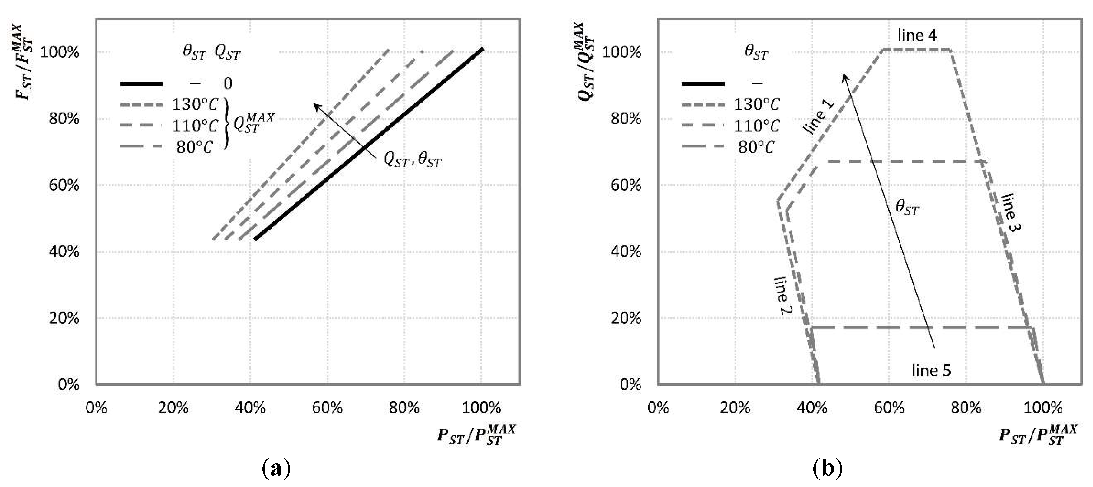
Figure 8.
Characteristic maps of the CHP combined cycle unit () for different generation ( ) and ambient () temperatures: (a) for and (b) map. For simplicity, the dependence on is shown only for .
Figure 8.
Characteristic maps of the CHP combined cycle unit () for different generation ( ) and ambient () temperatures: (a) for and (b) map. For simplicity, the dependence on is shown only for .
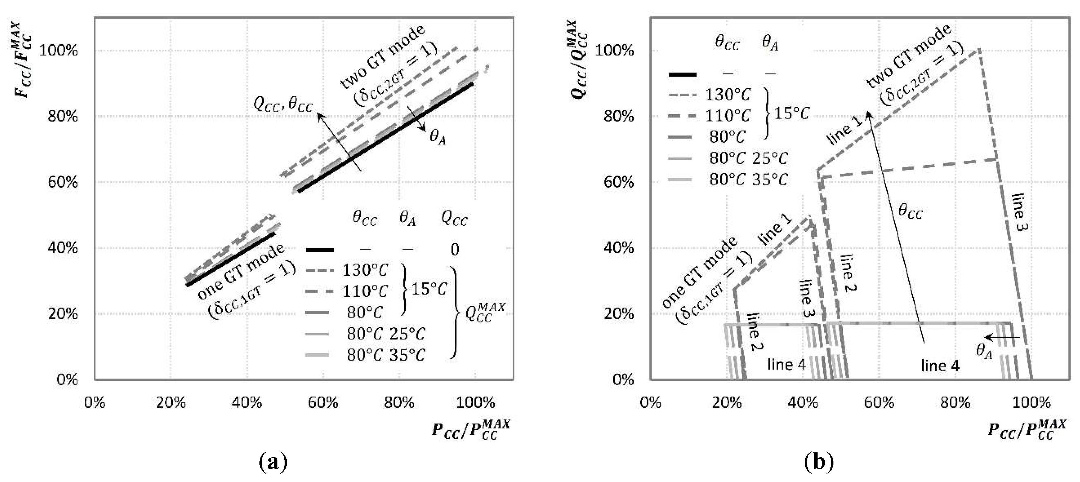
Figure 9.
Fleet of large-scale energy units serving a district heating network.

Figure 10.
Fleet of medium-scale energy units in a mountain resort.


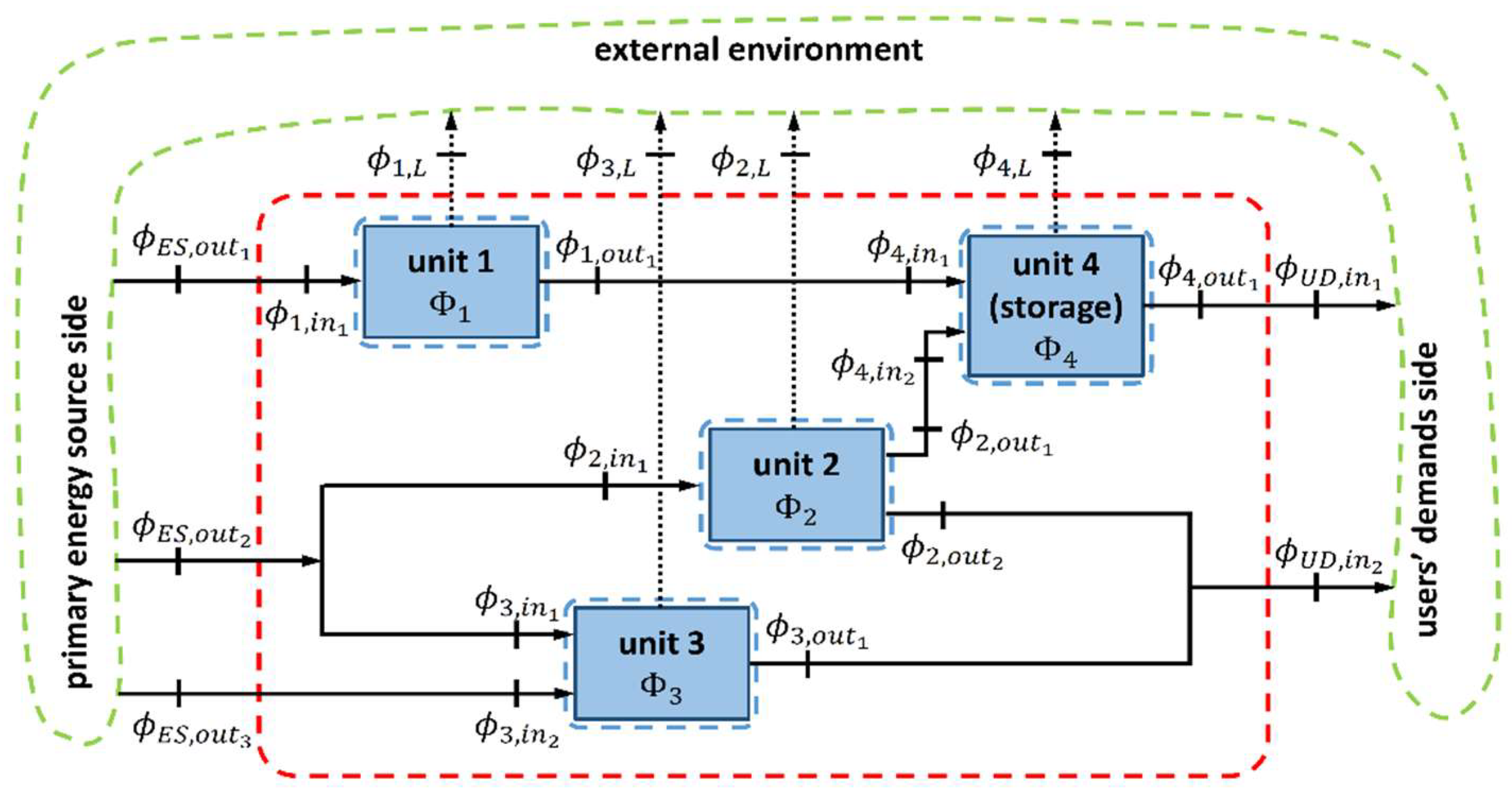
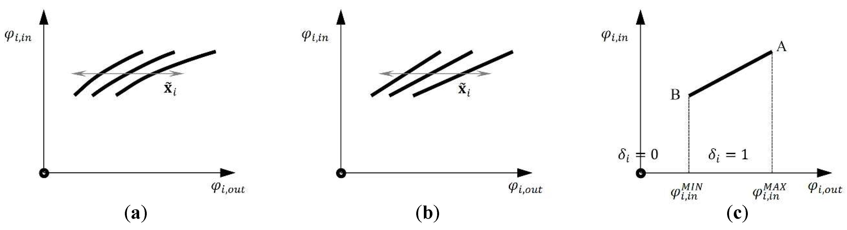
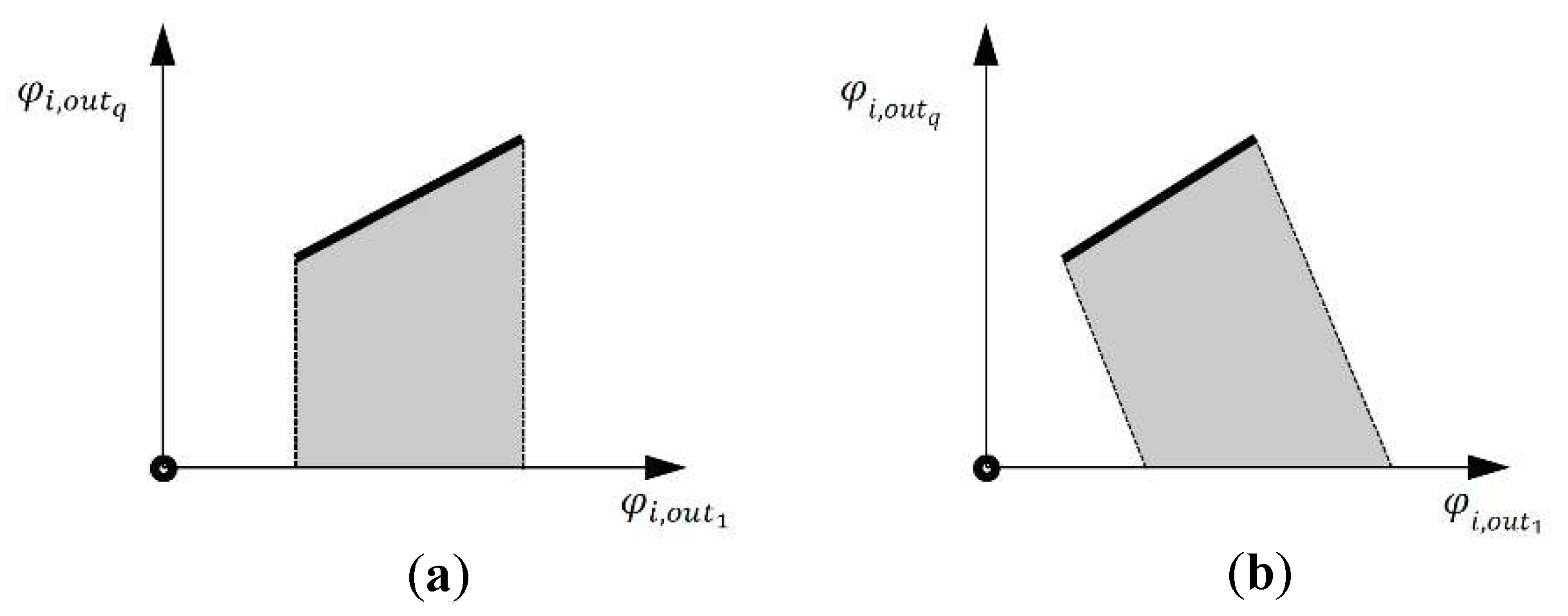
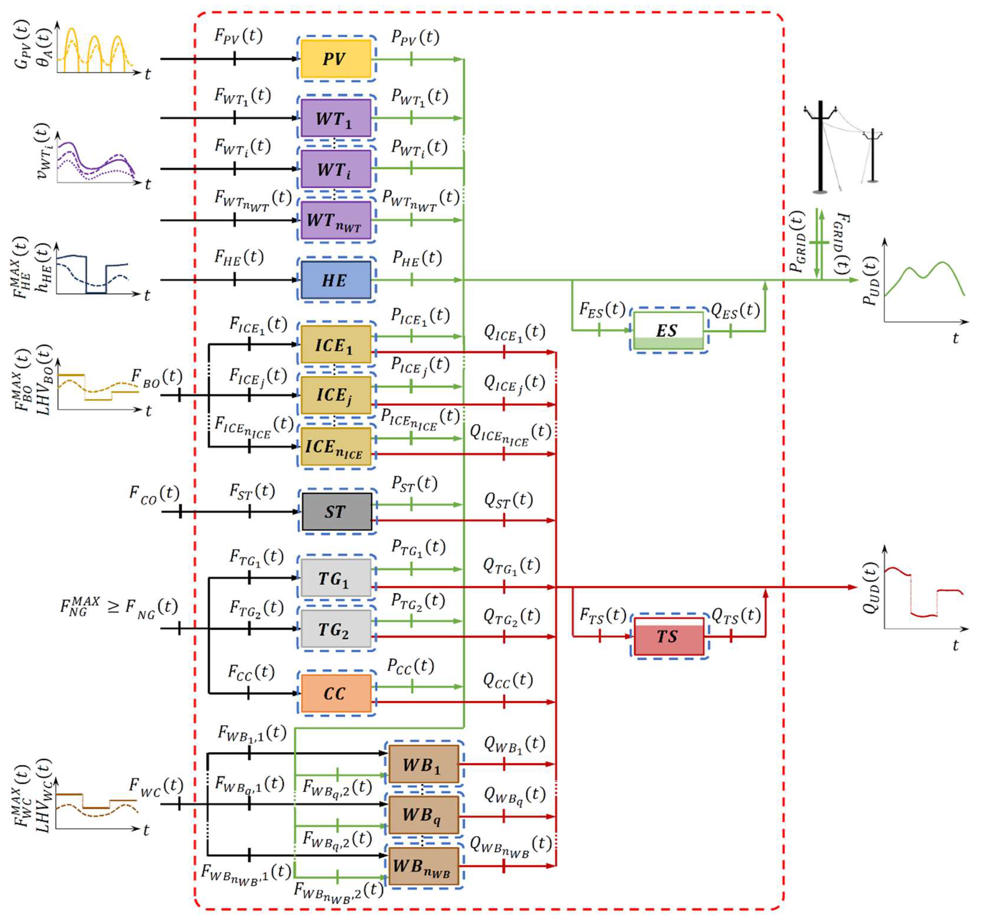
Table 1.
Equations of the dynamic model of the fleet of energy units in Figure 1.
Table 1.
Equations of the dynamic model of the fleet of energy units in Figure 1.
| Equation Category | Units | Equation | Reference |
|---|---|---|---|
| Balance equation at the interconnection between units | (i) | ||
| (ii) | |||
| Balance equation at the interconnection between units and environment | (iii) | ||
| (iv) | |||
| (v) | |||
| (vi) | |||
| (vii) | |||
| Balance equation expressing the energy conservation within the units | (viii) | ||
| (ix) | |||
| (x) | |||
| (xi) | |||
| Characteristic maps of the units | (xii) | ||
| (xiii) | |||
| (xiv) | |||
| (xv) | |||
| (xvi) | |||
| (xvii) |
Table 2.
Set of the decision variables in the optimization of the design and operation of the fleet of energy units in Figure 5.
Table 2.
Set of the decision variables in the optimization of the design and operation of the fleet of energy units in Figure 5.
| Symbols | Type | Description | U.M. | ||
|---|---|---|---|---|---|
| Optimization of the design and operation | ,,,, | Binary | Inclusion or not of the energy conversion units (except and ) in the optimum configuration | ||
| Real | Maximum capacity (size) of the photovoltaic power station (), and electric () and thermal () storage units | ||||
| Optimization of the operation only | ,,, ,,,, | Binary | On/off status of the energy conversion units (except and ) | ||
| ,,, ,, | Real | Electric power generated by the energy conversion units (except and ) | |||
| ,, ,, ,, , | Real | Electric power generated by the energy conversion units and sent to the electric grid | |||
| ,,, , | Real | Thermal power generated of the energy conversion units (except , and ) |
Table 3.
Input data in the optimization of the design and operation of the fleet of energy units in Figure 5.
Table 3.
Input data in the optimization of the design and operation of the fleet of energy units in Figure 5.
| Symbols | Type | Description | U.M. | |
|---|---|---|---|---|
| Optimization of the design and operation | Real | Electric and thermal power required by the users () | ||
| ,,, ,, | Real | Round-trip efficiency and oversizing/minimum capacity coefficients of the storage units | ||
| ,,,, ,, | Real | Maximum electric power output of the energy conversion units (except ) | ||
| Optimization of the design and operation | Real | Maximum thermal power output of the woodchip boilers () | ||
| Real | Electric power generated by the photovoltaic power station () per unit of nominal power (calculated from solar irradiance and ambient temperature , see Equation (34)) | |||
| Real | Electric power that each wind turbine () could produce (obtained from wind speed , see Equation (35)) | |||
| ,,,,, ,, | Real | Ratio between minimum and maximum load of the energy conversion units | ||
| ,, ,,, | Real | Constant parameters which multiply the binary variables in the characteristic maps of energy conversion units (, and ) | ||
| ,,, ,,, | Real | Variable parameters which multiply the binary variables in the characteristic maps of energy conversion units (, and ) (calculated from available water head or ambient temperature ) | ||
| ,,,,,,,,, ,,,,,, , | Real | Constant parameters which multiply an electric or thermal power output in the characteristic maps of energy conversion units (all except and ) | ||
| ,,, | Real | Variable parameters which multiply an electric or thermal power output in the characteristic maps of energy conversion units (, and ) (calculated from available water head or ambient temperature ) | ||
| , | Real | Time periods which define the type of start-ups in Equations (50) and (51) | ||
| Real | Number of hours required for start-ups | |||
| ,,, | Real | Maximum load ramp rates during normal operation and start-ups | ||
| Real | Minimum uptime and operating time of the energy conversion units (except , and ) | |||
| Optimization of the design and operation | Real | Available power associated with hydropower (), woodchips () and bio-oil () and natural gas () (calculate by Equations (23) and (24) from the corresponding mass flow rates) | ||
| Real | Maximum power associated with natural gas () (calculate by Equation (24) from the corresponding maximum mass flow rates) | |||
| , | Real | Historical or forecasted time profiles of ambient temperature and solar irradiance | ||
| , | Real | Historical or forecasted time profiles of available water head and wind speed | ||
| ,,,,,,, | Real | Variable energy prices, costs and premium feed-in tariffs | ||
| Real | Constant premium feed-in tariffs | |||
| Real | Annual tax credit per unit of installed capacity of the woodchip boilers () | |||
| Real | Annual operation and maintenance costs per unit of installed capacity of the energy conversion units | |||
| , | Real | Annual operation and maintenance costs per unit of installed capacity of the electric and thermal storage units | ||
| Real | CO2 emission per unit of fuel energy of the units converting fossil fuels | |||
| Real | Specific CO2 emission allowances cost | |||
| ,,,, ,,,, ,, | Real | Cost of the start-ups of the energy conversion units (except , and ) | ||
| Real | Annual amortization of purchase and installation costs of energy conversion units (except ) per unit of installed capacity | |||
| , | Real | Annual amortization of purchase and installation costs of the electric and thermal storage units per unit of storage capacity | ||
| Optimization of the operation only | ,,,, , | Binary | Inclusion or not of the energy conversion units (except and ) in the optimum configuration | |
| Real | Maximum capacity (size) of the photovoltaic power station (), and electric () and thermal () storage units |
Table 4.
Nameplate characteristics of the energy conversion units included in the system in Figure 9 at . For and units, refers to the total thermal power output () at the maximum temperature ().
Table 4.
Nameplate characteristics of the energy conversion units included in the system in Figure 9 at . For and units, refers to the total thermal power output () at the maximum temperature ().
| Unit | Supply Area | Manufacturer–Model | |||
|---|---|---|---|---|---|
| Siemens–SGT5-3000E (41MAC) 50 Hz | |||||
| , | Siemens–2 x SGT5-1000F 50 Hz | ||||
| Siemens–SGT-800 50 Hz | |||||
| General Electric–GE LM6000 PC Sprint 50 Hz |
Table 5.
Nameplate characteristics of the renewable energy conversion units included in the system in Figure 10 and peak thermal and electric power of the users.
Table 5.
Nameplate characteristics of the renewable energy conversion units included in the system in Figure 10 and peak thermal and electric power of the users.
| Unit | Type | Manufacturer–Model | ||||
|---|---|---|---|---|---|---|
| PV power station | modules: BP 3230T | |||||
| Hydroelectric plant | ||||||
| Bio-oil CHP ICE | MAN–D 2842 LE 211 | |||||
| Bio-gas CHP ICE | MAN–E 2848 LE 322 | |||||
| Woodchip boilers | ETA–Hack 200 | |||||
| Users (total) | 863.5 | 1785.0 |
© 2019 by the author. Licensee MDPI, Basel, Switzerland. This article is an open access article distributed under the terms and conditions of the Creative Commons Attribution (CC BY) license (http://creativecommons.org/licenses/by/4.0/).
Share and Cite
MDPI and ACS Style
Rech, S. Smart Energy Systems: Guidelines for Modelling and Optimizing a Fleet of Units of Different Configurations. Energies 2019, 12, 1320. https://doi.org/10.3390/en12071320
AMA Style
Rech S. Smart Energy Systems: Guidelines for Modelling and Optimizing a Fleet of Units of Different Configurations. Energies. 2019; 12(7):1320. https://doi.org/10.3390/en12071320
Chicago/Turabian StyleRech, Sergio. 2019. "Smart Energy Systems: Guidelines for Modelling and Optimizing a Fleet of Units of Different Configurations" Energies 12, no. 7: 1320. https://doi.org/10.3390/en12071320
Note that from the first issue of 2016, this journal uses article numbers instead of page numbers. See further details here.