A Process Integration Method for Total Site Cooling, Heating and Power Optimisation with Trigeneration Systems

Abstract

Research and development on integrated energy systems such as cogeneration and trigeneration to improve the efficiency of thermal energy as well as fuel utilisation have been a key focus of attention by researchers. Total Site Utility Integration is an established methodology for the synergy and integration of utility recovery among multiple processes. However, Total Site Cooling, Heating and Power (TSCHP) integration methods involving trigeneration systems for industrial plants have been much less emphasised. This paper proposes a novel methodology for developing an insight-based numerical Pinch Analysis technique to simultaneously target the minimum cooling, heating and power requirements for a total site energy system. It enables the design of an integrated centralised trigeneration system involving several industrial sites generating the same utilities. The new method is called the Trigeneration System Cascade Analysis (TriGenSCA). The procedure for TriGenSCA involves data extraction, constructions of a Problem Table Algorithm (PTA), Multiple Utility Problem Table Algorithm (MU PTA), Total Site Problem Table Algorithm (TS PTA) and estimation of energy sources by a trigeneration system followed by construction of TriGenSCA, Trigeneration Storage Cascade Table (TriGenSCT) and construction of a Total Site Utility Distribution (TSUD) Table. The TriGenSCA tool is vital for users to determine the optimal size of utilities for generating power, heating and cooling in a trigeneration power plant. Based on the case study, the base fuel source for power, heating and cooling is nuclear energy with a demand load of 72 GWh/d supplied by 10.8 t of Uranium-235. Comparison between conventional PWR producing power, heating and cooling seperately, and trigeneration PWR system with and without integration have been made. The results prove that PWR as a trigeneration system is the most cost-effective, enabling 28% and 17% energy savings as compared to conventional PWR producing power, heating and cooling separately.

1. Introduction

Rapid industrialisation and rising global population contribute to the rapid depletion of energy resources, environmental pollution and climate change. The International Energy Agency [1] has predicted increasing CO₂ emissions from 0.15 × 10¹² MWh in 2008 to 0.23 × 10¹² MWh in 2035 as well as a rising crude oil price from 60 USD/barrel in 2011 to 120–140 USD/barrel from 2020 onwards. These challenges have become the key drivers to improve the energy efficiency of power plants. Zhang et al. [2] summarised strategies to reduce greenhouse gas emissions that include utilisation of a mixture of energy generation technologies in one location, development of highly-efficient energy production and re-use methods as well as implementing the use of incentives, technologies, taxes and quotas. Abdul Manan et al. [3], on the other hand, proposed a methodology that provides clear visualisation insights for CO₂ emission planning as well as good target estimation for problems involving resource planning and conservation towards achieving cleaner production goals. Implementation of integrated energy systems such as cogeneration and trigeneration systems as a centralised power plant can improve its energy efficiency by reuse of waste heat produced for other applications such as distillation process, district heating and cooling. Cogeneration systems, which are also known as Combined Heating and Power (CHP) systems is a technology whereby electricity and heat are produced simultaneously from a single fuel source. Trigeneration systems, on the other hand, are an advanced cogeneration system technology which produces cooling, heating and electricity at the same time from a primary source of energy. Production of cooling by using absorption chillers is an advantage in a trigeneration system. Khamis et al. [4] stated that an improvement in energy efficiency could translate into lower operating cost, reduced emissions and reduced usage of fossil fuels.

Process Integration (PI) is a process to reduce the consumption of resources as well as environmental emissions. Pinch Analysis (PA) is one of the PI methodologies which has been widely applied for designing and obtaining optimal targets for various resource conservation networks. Recent studies show that various resources proposed for PA such as heat, water, mass, carbon, property and gas were progressively developed, see Klemeš et al. [5]. The progressive development of PA in various resource networks proved that the methodology had gained acceptance by the public due to its simple insightful approaches using graphical or numerical techniques. The latest studies related to Power Pinch Analysis (PoPA) approaches have been included in this paper. PoPA which is introduced by Wan Alwi et al. [6] helps designers obtain the amount of excess electricity as well as minimum targets for outsourced electricity. Mohammad Rozali et al. [7] extended the application of PoPa by including losses analysis associated with power conversion, transfer and storage. Ho et al. [8] proposed a new numerical method based on PoPA approaches which were called Electricity System Cascading Analysis (ESCA). The method is developed for designing and optimising non-intermittent power generator such as biomass, biogas, natural gas, nuclear and diesel as well as energy storage systems. Liu et al. [9] combined both methods developed by Mohammad Rozali et al. [7] and Ho et al. [8] to obtain optimal design and sizing of multiple decentralised energy systems and a centralised energy system. Jamaluddin et al. [10] then extended the PoPA method from Mohammad Rozali et al. [7] to determine the minimum targets for outsourced power, heating and cooling, amount of excess power, heating and cooling during the first day as well as for continuous 24 h operations simultaneously; and to determine the maximum storage capacity in a trigeneration system. Jamaluddin et al. [11] then included safety considerations in PoPA for designing safe and resilient hybrid power systems. Recent studies had been done by Hoang et al. [12] to obtain an optimal hybrid renewable energy system which can sustainably meet the electricity demand by using the PoPA method.

Initially, Dhole and Linnhoff [13] introduced Total Site Integration of industrial systems. The Total Site Integration concept developed by Dhole and Linnhoff [13] is based on the ideas of the Site Heat Source and Site Heat Sink. Total Site Heat Integration (TSHI), developed by Klemeš et al. [14], is a tool which focuses on integrating heat at multiple sites. TSHI can be very beneficial in terms of cost effectiveness since the new and existing plant piping systems can be used to indirectly transfer heat through utility systems. The concept of Total Site was extended by Perry et al. [15] to a broader spectrum of processes in addition to the industrial process. Integration of renewable energy sources was included in the analysis to reduce the carbon footprint of a Locally Integrated Energy Sector (LIES). Heat sources and sinks from small scale industrial plants, offices, residential areas and large building complexes such as hotels and hospitals can be analysed by using LIES. Matsuda et al. [16] applied Total Site Integration in a number of chemical industrial sites and heterogeneous Total Site involving a brewery and several commercial energy users. Varbanov and Klemeš [17] improved the concept of Total Site by introducing a set of time slices to meet the variation of energy supply and demand. Varbanov and Klemeš [18] then extended the Total Site concept by including heat storage, waste heat minimisation and carbon footprint reduction as well as the Total Site heat cascade. Next, Liew et al. [19] introduced a new numerical approach to allow designers and engineers to assess the sensitivity of a whole site with respect to operational changes using a Total Site Sensitivity Table (TSST) as well as to assess the impact of sensitivity changes on a cogeneration system, determine the optimum utility generation system size, assess the need for backup piping and estimate the amount of external utilities needed. Total Site Integration can also be extended to cogeneration targeting. Shamsi and Omidkhah [20] developed a thermo-economically-based approach for optimisation of steam levels in steam production as well as reduction of total cost of the utility system in Total Site. Chew et al. [21] extended TSHI by including pressure drop on utility. Klemeš et al. [22] reviewed Total Site Integration methodologies on cogeneration. The representation of cogeneration potential has been firstly documented by Raissi [23]. Site Utility Grand Composite Curve (SUGCC) developed by Klemeš et al. [14] allows thermodynamic targets for cogeneration with targets for site-scope Heat Recovery minimising the cost of utilities. Varbanov et al. [24] introduced improvements to the model of back-pressure steam turbine performance. Boldyrev et al. [25] calculated capital cost assessment for power cogeneration and evaluated the potential steam turbine placement for various steam pressure levels. Liew et al. [26] later improved the TSST for planning the TSHI centralised utility system. Liew et al. [27] further improved the methodology by incorporating absorption and electric chillers. A new TSHI is proposed by Tarighaleslami et al. [28] to optimise both non-isothermal and isothermal utilities. Ren et al. [29] then proposed a simulation to target the cogeneration potential of Total Site utility systems. Recent studies proposed by Pirmohamadi et al. [30] to obtain the optimum design of cogeneration systems in Total Site by using exergy approach.

A numerical tool based on PA approach called Problem Table Algorithm (PTA) was developed by Linnhoff and Flower [31] for intra-process heat integration. This tool has the same application as the Composite Curves and Grand Composite Curve but provides more accurate values for the Pinch Points. Costa and Queiroz [32] extended the concept of PTA by implementing multiple utility targets. Unified Targeting Algorithm (UTA) proposed by Shenoy [33] is used as a powerful tool to determine maximum resource recovery for PI. The methods proposed by Costa and Queiroz [32] and later by Shenoy [33] had a weakness. The UTA developed by Shenoy [33] cannot be used for TSHI problems whereas the method developed by Costa and Quiroz [32] involves complex calculations. Liew et al. [19] developed a new numerical for targeting TSHI which known as the Total Site Problem Table Algorithm (TS-PTA) to tackle the weaknesses in Costa and Quiroz’s approach [32] and Shenoy’s [33] works. The methodology has been improved by including time slide due to variation on demands and sources [26], absorption and electric chillers for production of chilled water [27] and incorporating long and short terms heat energy supply and demand variation problem [34].

Until now, the published extensions of Pinch Analysis have yet to provide a complete solution for trigeneration systems. The Total Site Heat Integration should be extended for Cooling, Heating and Power (TSCHP), and the benefits of power, heating and cooling targeting related to the actual trigeneration system design need to be emphasised. The objective of this work is to develop an insight-based numerical Pinch Analysis methodology to minimise the heating, cooling and power requirements as well as to determine the capacity of energy storage systems of a trigeneration system for TSCHP. The intermittency from the demands can greatly affect the performance of the system because the energy should be continuously produced and supplied based on demand needs. The development of this systematic methodology is very important for users to determine allocation and targets of power, heating and cooling in a trigeneration system as well as to optimise the trigeneration system.

2. Methodology and Case Study

Trigeneration System Cascade Analysis (TriGenSCA) is a new numerical method being developed in this paper to minimise power, heating and cooling targeting as well as to optimise sizing of the turbine, absorption chiller, cooling tower and steam generator. TSCHP integration method is an extension of TSHI which focuses on intra-processes of integrating heating, cooling and power for multiple sites. Summary of the overall methodology of this paper is shown in Figure 1. Based on the figure shown, the overall methodology can be categorised into eight steps which are data extraction, Problem Table Algorithm (PTA) [19] for an individual process, Multiple Utility Problem Table Algorithm (MU-PTA) [19] for an individual process, Total Site Problem Table Algorithm (TS-PTA) for all processes, estimation of energy source from trigeneration system, Trigeneration System Cascade Analysis (TriGenSCA), Trigeneration Storage Cascade Table (TriGenSCT) and Total Site Utility Distribution (TSUD) to obtain optimal size of trigeneration system.

The trigeneration system is implemented as a centralised energy system to supply power, heating and cooling applications to the demand as shown in Figure 2. Based on the figure shown, Very High-Pressure Steam (VHPS) is produced from steam generator (acting as the same function as a boiler) and passes through a double extraction turbine simultaneously producing power and lower pressure steams such as High-Pressure Steam (HPS) and Low-Pressure Steam (LPS). The HPS which is produced from the double extraction turbine can be supplied to meet the demands directly or stepped down to LPS using a relief valve. Excess HPS and LPS can be cooled down by using CW or condensed by using the condensing turbine to generate more power. Condensing turbines have an advantage whereby they can adjust their electrical output by altering the proportion of steam passing through the turbine. Hot Water (HW), on the other hand, is generated by using the condensation system. HW can then be used either directly to the demand or converted to cooling utilities such as Cooling Water (CW) and Chilled Water (ChW). CW is produced through the cooling tower and ChW by using an absorption chiller.

The cooling tower is generally used to cool process water via evaporation [35]. Operation of cooling tower starts with HW is pumped to enter at the top through nozzles. The HW flowing through the nozzles is dispersed onto a large surface area which is also known as a fill. The fill is used to delay water from reaching the bottom of the tower and allow more time for the air to interact with the HW. The water then slowly makes its way through the fill tanks via gravity and a fan forces air across the water path until it reaches the bottom of the tower. CW is then produced at the bottom of the tower and supplied to the demands. The absorption chiller, on the other hand, consists of four main components which are generator, condenser, evaporator and absorber [36]. The process of producing of ChW by using absorption chiller is summarised below:

1)

Generator—the HW produces refrigeration vapour from a strong refrigerate solution by transferring heat from HW to coll the solution. The refrigeration vapour needs to pass through a rectifier for dehydration before it enters the condenser.

2)

Condenser—dehydrated and high-pressure refrigerant enters the condenser where it is condensed. The refrigerant goes through an expansion valve after cooling. Expansion valve reduces the pressure and temperature of the refrigerant. The new values of refrigerant must be below than in evaporator.

3)

Evaporator—the cold refrigerated space is appearing in the evaporator. The cooled refrigerant enters the evaporator, absorbs heat and then leaves as saturated refrigeration vapour.

4)

Absorber—the refrigeration vapour exposed to a spray of the weak refrigerant-absorbent solution. The weak solution changes to a strong solution. The new solution passes through regenerator which is also known as a heat exchanger. The solution arrives at the generator has the same pressure as before. The process is then repeated.

Some simplifying assumptions are listed below:

(i)

Energy loss due to transmission has not been considered at this stage.

(ii)

Energy loss from storage system is considered where the lead-acid battery is used as a power storage system with charging and discharging efficiencies of 90% [37]. Thermo-chemical storage, on the other hand, is used as a heating and cooling thermal storage systems with charging and discharging efficiencies of 58% [38]. Conversions of power from AC to DC and from DC to AC are also considered with an inverter efficiency at 90% [37].

(iii)

Energy conversion is taken into consideration where the efficiency of double extraction turbine is assumed to be 25% [39], the efficiency of condensing turbine is 33% [40], the efficiency of the condensation system is 30% [41], and the efficiency of the cooling tower and absorption chiller are 30% [42].

(iv)

Trigeneration system and industrial plants are in continuous 24 h operations, and fluctuation due to weather change and demands have not been accounted for.

(v)

Energy consumption remains unchanged regardless of changes of the topology in the industrial plants.

2.1. Step 1: Data Extraction

In the first step, the local energy supply and demand data of the trigeneration system and industrial plants are needed. The data extraction is separated into two sides which are power and heating/cooling sides. Figure 3 shows the hourly average electricity demands for four industrial. Figure 4 summarises the total electricity demands for the four industrial plants.

Meanwhile, heating/cooling data extraction requires a supply temperature, T_s, target temperature, 10 °C T_t, the minimum temperature difference between utility and process streams, ΔT_min,up and minimum flowrate heat capacity, mCP. The difference in enthalpy ΔH is obtained using Equation (1):

$$\Delta H=mCP\times (T_s-T_t)$$

(1)

where ΔH = the difference in enthalpy in MW; mCP = Minimum flowrate heat capacity in MW/°C; supply temperature in °C; T_t = Target temperature in °C.

Stream data for four industrial plants are obtained from Perry et al. [15] and has been modified. The stream data for four industrial plants are shown in

Table 1. Stream data for Industrial Plant A with ΔT_min,pp 20 °C [19].

Stream	Ts (°C)	Tt (°C)	ΔH (MW)	mCP (MW/°C)	Ts’ (°C)	Tt’ (°C)
A1 Hot	170	80	5	0.06	160	70
A2 Hot	150	55	6.48	0.07	140	45
A3 Cold	25	100	15	0.2	35	110
A4 Cold	70	100	1.05	0.04	80	110
A5 Cold	30	65	5.25	0.15	40	75

,

Table 2. Stream data for Industrial Plant B with ΔT_min,pp 10 °C [19].

Stream	Ts (°C)	Tt (°C)	ΔH (MW)	mCP (MW/°C)	Ts’ (°C)	Tt’ (°C)
B1 Hot	200	20	0.0005	0.08	195	15
B2 Cold	10	100	4	0.04	15	105
B3 Cold	100	120	10	0.5	105	125
B4 Hot	150	40	8.443	0.08	145	35
B5 Cold	60	110	1	0.02	65	115
B6 Cold	75	150	7	0.09	80	155

,

Table 3. Stream data for Industrial Plant C with ΔT_min,pp 20 °C [19].

Stream	Ts (°C)	Tt (°C)	ΔH (MW)	mCP (MW/°C)	Ts’ (°C)	Tt’ (°C)
C1 Hot	85	40	225	5	75	30
C2 Hot	80	40	400	10	70	30
C3 Hot	41	38	105.3	35.1	31	28
C4 Cold	25	65	23.6	0.59	35	75
C5 Cold	55	65	25.8	2.58	65	75
C6 Cold	33	60	6.48	0.24	43	70
C7 Cold	25	60	77	2.2	35	70
C8 Cold	30	240	29.4	0.14	40	250
C9 Cold	25	28	150	50	35	38
C10 Cold	30	100	59.5	0.85	40	110
C11 Cold	18	50	224	7	28	60
C12 Cold	21	200	8.95	0.05	31	210

and

Table 4. Stream data for Industrial Plant D with ΔT_min,pp 10 °C [19].

Stream	Ts (°C)	Tt (°C)	ΔH (MW)	mCP (MW/°C)	Ts’ (°C)	Tt’ (°C)
D1 Cold	15	60	149.85	3.33	20	65
D2 Cold	15	80	515	7.92	20	85

. Calculation of shifted temperatures for the process streams in each individual process are necessary where temperatures of cold streams, T_c, are shifted to perform shifted cold stream temperatures (T_c’) by adding half of the minimum temperature between processes, ΔT_min,pp, whereas the temperatures of hot streams, T_h, are shifted to perform shifted hot stream temperatures (T_h’) by reducing half of the ΔT_min,pp. The value of ΔT_min,pp for Plants A and C is assumed to be 20 °C whereas ΔT_min,pp for Plants B and D are assumed to be 10 °C [19]. Multiple utility temperature levels data available at the plants is described in

Table 5. Stream data for Industrial Plant D with ΔT_min,pp 10 °C [19].

Multiple Utilities	Temperature (°C)
HPS	240
LPS	150
HW	50
CW	20
ChW	10

.

2.2. Step 2: Construct Problem Table Algorithm (PTA) for Each Plant

Heating and cooling streams data need to be further analysed by using PTA. PTA is a numerical method proposed by Linnhoff and Flower [31] to obtain Temperature Pinch Point, minimum external heat, QH_min and minimum external cold, QC_min, required. The PTA has similar functions as Composite Curves (CCs) and Grand Composite Curves (GCCs) in a graphical approach and also provides more precise values at crucial points. For details on the construction of PTA, readers may refer to Linnhoff and Flower [31]. Tables S1–S4 (in Supplementary) Material show completed PTA on Plants A to D. The construction of PTA is shown below:

1)

Column 1 presents shifted temperature in descending order which is obtained from Step 1 whereas Column 2 shows temperature intervals.

2)

Column 3 shows minimum heat capacity from Step 1. Downside arrow represents a hot stream which is a positive value whereas upside arrow represents cold stream which is a negative value. On the other hand, Column 4 presents the cumulative minimum heat capacity obtained from Column 3.

3)

Column 5 shows total enthalpy between temperature interval which shown in Equation (2). Enthalpy represents energy cumulated in the steam:

$$\Delta H=mCP\times \Delta T$$

(2)

where ΔH = Total enthalpy between temperature interval; mCP = minimum heat capacity; ΔT = Temperature intervals.

4)

Single utility heat cascade shown in Column 7 follows the same equation as in Equation (3). The initial value is taken from the highest negative value in initial heat cascade (from Column 6) but make the value in positive. Values of QH_min and QC_min are obtained from the first and last row of Column 7.

$$H_i=H_{i-1}+\Delta H$$

(3)

where H_i = Current initial heat; H_i–1 = Previous initial heat; ΔH = Total enthalpy on temperature interval.

5)

Single utility heat cascade shown in Column 7 follows the same equation as in Equation (3). The initial value is taken from the highest negative value in initial heat cascade (from Column 6) but make the value in positive. Values of QH_min and QC_min are obtained from the first and last row of Column 7.

PTA results are summarised in

Table 6. Summary of PTA for Industrial Plants A to D.

	Plant A	Plant B	Plant C	Plant D
QHmin (MW)	9.82	4.30	61	664.85
QCmin (MW)	0	5.74	111.42	0
Temperature Pinch Point	35 °C	105 °C	75 °C	20 °C

. Based on Table 6, Temperature Pinch Points of all industrial plants are obtained. The Temperature Pinch Point for Plants A, B, C and D are 35 °C, 105 °C, 75 °C and 20 °C. The Temperature Pinch Point will be used in the next step. Meanwhile, the value of QH_min in Plant A is 9.82 MW and minimum external cold required is unnecessary as the value of QC_min is zero. Plant B, on the other hand, requires 4.30 MW and 5.74 MW of QH_min and QC_min. Value of QH_min for Plants C and D are 61 MW and 664.85 MW and value of QC_min for Plant C is 111.42 MW. Minimum external cooling for Plant D is unnecessary.

2.3. Step 3: Construct the Multiple Utility Problem Table Algorithm (MU PTA) for Each Plant

MU-PTA developed by Liew et al. [19] is an extension of PTA where four columns are added to target the amounts of various utility levels selected as potential sinks and sources for use in TSCHP. MU PTA has been used to identify pockets and target the exact amounts of utilities required within a given utility temperature interval. Multiple utility cascades are performed in two separate regions which are above and below regions of the Temperature Pinch Point obtained from Step 2 for each plant. For further details on the construction of MU PTA readers may refer to Liew et al.’s [19] work. Tables S5–S8 show MU PTA for all industrial plants.

2.3.1. Multiple Utility Cascades in the Region above the Pinch of Each Plant

At the above region of the Pinch Point, all shifted temperatures (T’) are reduced by ΔT_min,pp/2 for returning the temperature back to normal and ΔT_min,up is added, as shown in Column 2 (in Supplementary Material). The resulting temperature is shown as T”. The temperature for multiple utility shown in Table 5 is added to Column 2 as well. Implementation of multiple utility temperature in Column 2 will ease the user to determine the utility distribution at a later stage.

Columns 3 until 6 follow the same method as shown in Step 2. Column 7 shows heat is cascaded from the highest temperature to the temperature Pinch Point. The cascading is different as compared with that in Step 2 because the cascading process is done interval-by-interval. The external utility is immediately added as soon as a negative value is encountered. This cascading process is known as ‘multiple utility heat cascade’. The amount of external utility added is listed in Column 8 where the amount of external utility is equal to the negative value in Column 7. Once the amount of external utility is added, heat cascade in Column 7 becomes zero. The procedure is then repeated until reach to the Pinch Temperature.

The amounts of each type of utility consumed can be obtained once the multiple utility heat cascades are completed. The heat utility sink or source is shown in Column 9 is obtained by adding the utility consumed below the utility temperature before the next utility temperature.

2.3.2. Multiple Utility Cascades in the Region below the Pinch of Each Plant

The same methodology is used for multiple utility cascading below the Pinch temperature. Below the Pinch region, all shifted temperatures (T′) are added ΔT_min,pp/2 and ΔT_min,up subtracted from them to obtain the temperatures in the utility temperature scale. Multiple utilities are also added in Column 2. Multiple utilities in Column 7, however, start from the bottom temperature to the Pinch temperature. Positive heat value must be zeroed out by generating utilities. Negative values are encountered during multiple utility cascading, as shown in Column 8, and they represent pockets in the GCC.

The amount of utility can be obtained by addition of the amounts of excess heat from above the utility temperature to the next utility temperature level. Column 9 presents the amounts of utility based on different utility temperature.

A summary of MU PTA for all industrial plants is shown in

Table 7. Summary of MU PTA for Industrial Plants A to D.

Utility	Plant A	Plant B	Plant C	Plant D
HPS	0 MW	0 MW	17 MW	0 MW
LPS	5.66 MW	4.30 MW	44 MW	327.26 MW
HW	4.16 MW	−3.23 MW	−100.7 MW	337.59 MW
CW	0 MW	−2.32 MW	−117 MW	0 MW
ChW	0 MW	−0.19 MW	0 MW	0 MW
Temperature Pinch Point	35 °C	105 °C	75 °C	20 °C

. Based on Table 7, Plant A required 5.66 MW of LPS and 4.16 MW of HW as a heat sink to the streams. Plant B required 4.30 MW of LPS as a heat sink to the streams whereas heat source in the form of HW is generated which has a value of 3.23 MW. CW and ChW also in a deficit by 2.32 MW and 0.20 MW to cool down the streams. Plant C required 17 MW of HPS as a heat sink to the streams whereas Plants C and D needed 44 MW and 327.26 MW of LPS as a heat sink. 100.7 MW of HW in Plant C is in surplus whereas Plant D required 337.59 MW of HW. CW in Plant C is in deficit by 117 MW.

2.4. Step 4: Construct Total Site Problem Table Algorithm (TS PTA)

Development of TS PTA is an extension of PTA where this step represents the site CC in Total Site. TS PTA, proposed by Liew et al. [19], is used to determine the amounts of utilities which can be exchanged among processes.

Table 8. TS PTA for all industrial plants.

1	2	3	4	5	6	7	8	9
Utility	Utility Temperature (°C)	Net Heat Source (MW)	Net Heat Sink (MW)	Net Heat Requirement (MW)	Initial Heat Cascade	Final Single Heat Cascade	Multiple Utility Heat Cascade	External Utility Requirement (MW)
					0	636.04	0
HPS	240	0	17	−17				17
					−17	619.04	0
LPS	150	0	381.22	−381.22				381.22
					-398.22	237.82	0
HW	50	103.93	341.75	−237.82				237.82
					−636.04	0	0	Pinch
CW	20	119.32	0	119.32				−119.32
					−516.72	119.32	0
ChW	10	0.197	0	0.197				−0.197
					−516.52	0.197	0

shows the completed development of TS PTA in industrial plants. The utilities obtained from Step 3 is arranged from highest to lowest temperature as presented in Column 2. The utilities generated below the Pinch Temperature in Step 2 are added as a net source as shown in Column 3. Meanwhile, utilities consumed above the Pinch temperature in Step 2 are determined as a net sink as shown in Column 4. Net heat requirement in Column 5 is the subtraction of net heat source with the net heat sink. A negative value of the net heat requirement represents a heat deficit whereas a positive value represents a heat surplus. Column 6 shows cascading of heat transferred from higher to lower temperatures which follows the Second Law of Thermodynamics. The heat surplus at a higher temperatures utility can be cascaded to heat deficits at a lower temperature utility. The initial heat cascade is started from zero, and the net heat requirement is cascaded from top to bottom. The most negative value in Column 6 is used to investigate the amount of external heat utility required for the system by making it positive and cascading the net heat requirement again as shown in Column 7. The Total Site Pinch Point can be obtained where the zero value is the Pinch point location in this column.

The utilities can be separated into two parts which are regions above and below the Total Site Pinch Point. The same methods as Step 3 are used and shown in Columns 8 and 9 were at above Total Site Pinch Point, net heat requirement (in Column 5) is cascaded from the top to the Pinch Point by assuming no external heat supplied at a temperature above the HPS. The same amount of external heating utility is added in Column 9 as there is a negative value in the cascade. Below region of Total Site Pinch Point, net heat requirement of multiple utilities is cascaded from the bottom to the Pinch Point. Cooling utilities are added as there is a positive value in the cascade until it reaches zero and represented by negative numbers.

2.5. Step 5: Estimation of Energy Source from a Trigeneration System

In this step, the energy source from a trigeneration system is preliminarily estimated to show values of energy required to supply to the demands. Various fuels such as coal, natural gas, diesel and nuclear as well as renewables can be applied in trigeneration systems. In this work, nuclear energy is suggested as a trigeneration system fuel since it is zero CO₂ emissions. Nuclear energy is a good supplier of energy for non-electrical applications such as heating and cooling processes for the same reason as electricity [4]. Figure 5 shows the range of applicability for nuclear reactors. Double extraction turbine requires the maximum steam temperature of 275.6 °C to generate power [39]. A Water Cooled Reactor (WCR) is thus chosen as the best nuclear reactor because it has the highest temperature of 320 °C. Pressurised Water Reactor Nuclear Power Plant (PWR NPP) is one of the types of WCR. Uranium-235 is used as a fuel to generate nuclear energy for PWR NPP.

Taking PWR NPP as a trigeneration system, calculation for power rating in the source is shown in Equation (4). The total daily power consumption is 4068 MWh/day (from Figure 4). The total power consumption is the cumulative power rating in a day. Generation of power from trigeneration system is assumed to be 169.5 MW and operate in 24 h since the nuclear power plant is a stable system:

$$P{E}_g=\frac{{{\displaystyle \sum PE}}_c}{T}$$

(4)

where PE_g = Average power generation in MW; ${{\displaystyle \sum PE}}_c$ = Total power consumption in MWh; T = total time in h.

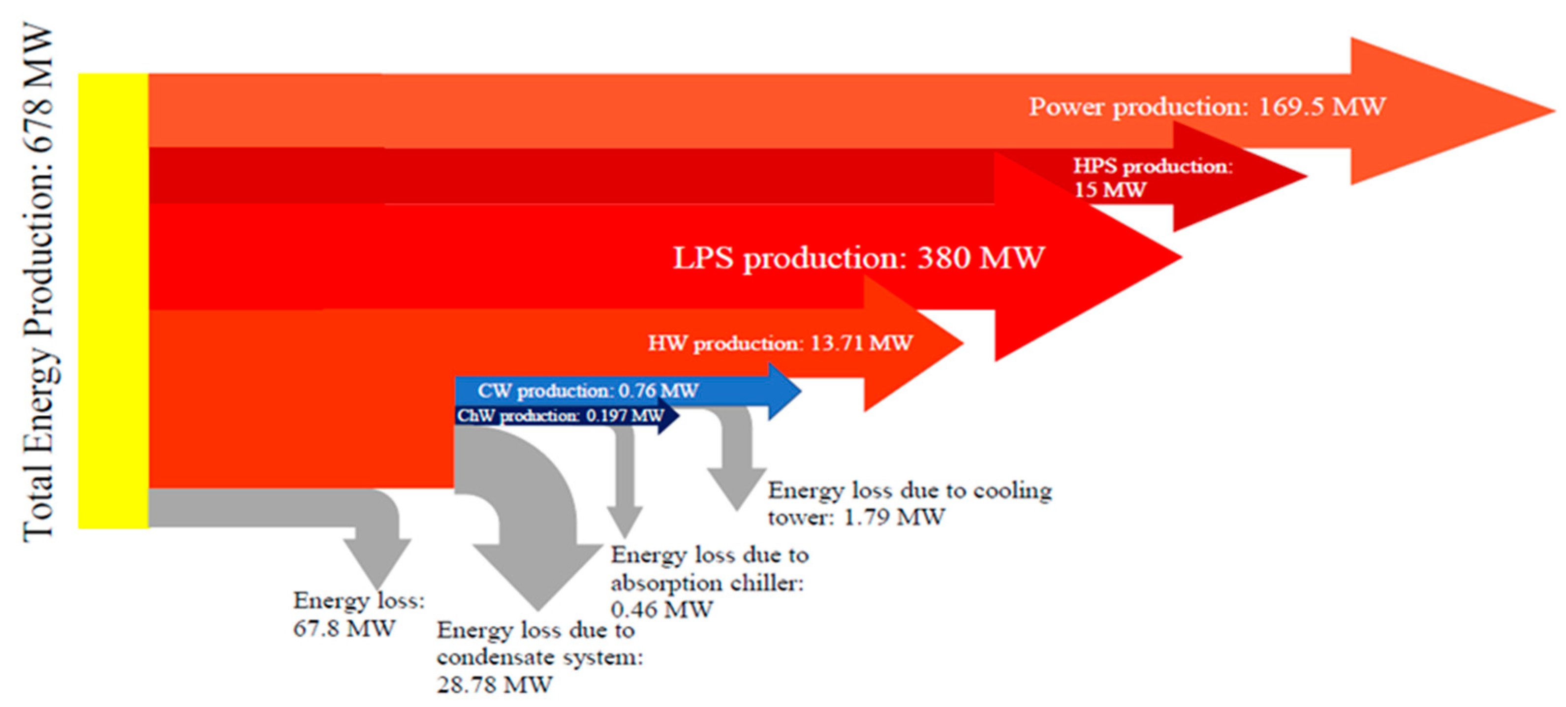
Total thermal energy produced by the trigeneration system then can be estimated based on power generation, PE_g. Equation (5) shows the estimation of total thermal energy produced by the trigeneration system. Average power generation for the trigeneration system is 169.5 MW and double extracting turbine efficiency is assumed to be 25% [39]. Based on a calculation by using Equation (5), the total thermal energy produced by the steam generator is 678 MW. The total thermal energy produced by the steam generator does not include any additional energy from extra fuel. This means that all production of Very High-Pressure Steam (VHPS) is used directly to the turbine without undergo relief valve to the lower temperature of utilities:

$${\displaystyle \sum TE=\frac{P{E}_g}{{\mu }_t}}$$

(5)

where $\sum TE$ = Total thermal energy produced by trigeneration system in MW; PE_g = Average power generation in MW; μ_t = Double extracting turbine efficiency.

Remaining waste energy can be determined by using Equation (6) and energy losses are assumed to be 10% [44]. Based on Equation (6), the remaining waste energy is 440.7 MW:

$$E_{waste}=TE-P{E}_g-(TE\times 10\%)$$

(6)

where E_waste = Remaining waste energy in MW; PE_g = Average power generation in MW; TE = total thermal energy produced by the trigeneration system in MW.

The division of remaining waste thermal energy produced by the trigeneration system is based on the highest temperature of utilities to the lowest temperature of utilities. The remaining waste energy produced by the trigeneration system starts with HPS and follows with LPS and HW. This means that 440.7 MW is divided into; (1) 15 MW of HPS, (2) 380 MW of LPS and (3) remaining 45.7 MW of waste heat which will be converted into HW by using the condensation system. Taking efficiency of condensation system into consideration, 13.71 MW of HW is produced from 45.7 MW of waste heat. Out of 13.71 MW, 10.5 MW can be used directly to meet demands whereas the remaining 3.21 MW of HW can be converted into CW and ChW through the cooling tower and an absorption chiller. Production of 0.197 MW of ChW from absorption chiller requires 0.657 MW of HW and the remaining 2.553 MW of HW can produce 0.7659 MW of CW by using the cooling tower by taking the values of the absorption chiller and cooling tower efficiencies which are 30% into account. Figure 6 shows a summary of the energy that is formed by the trigeneration system.

2.6. Step 6: Trigeneration System Cascade Analysis (TriGenSCA)

TriGenSCA is introduced in this paper to further target the minimum power, heating and cooling as well as to optimise the size of utilities in trigeneration system considering storage system is available to store surplus energy at one time and utilise when there is deficit energy requirement. The construction of TriGenSCA consists of three major steps which are cascade analysis, calculation of the new size of the trigeneration system and percentage change between previous and new trigeneration system size.

2.6.1. Cascade Analysis

Cascade analysis is the first step in developing TriGenSCA. The cascade analysis is used to verify the estimated size of utilities in trigeneration system.

Table A1. TriGenSCA before iteration from time 1 to 12 h.

1	2						3
Time (h)	Demand (MW)						Generation (MW)
	Power	Heating			Cooling		Power	Heating			Cooling
		HPS	LPS	HW	CW	ChW		HPS	LPS	HW	CW	ChW
1	120	17	381.22	237.82	119.32	0.197	169.5	15	380	10.5	0.76	0.197
2	123	17	381.22	237.82	119.32	0.197	169.5	15	380	10.5	0.76	0.197
3	180	17	381.22	237.82	119.32	0.197	169.5	15	380	10.5	0.76	0.197
4	230	17	381.22	237.82	119.32	0.197	169.5	15	380	10.5	0.76	0.197
5	125	17	381.22	237.82	119.32	0.197	169.5	15	380	10.5	0.76	0.197
6	95	17	381.22	237.82	119.32	0.197	169.5	15	380	10.5	0.76	0.197
7	145	17	381.22	237.82	119.32	0.197	169.5	15	380	10.5	0.76	0.197
8	169	17	381.22	237.82	119.32	0.197	169.5	15	380	10.5	0.76	0.197
9	202	17	381.22	237.82	119.32	0.197	169.5	15	380	10.5	0.76	0.197
10	205	17	381.22	237.82	119.32	0.197	169.5	15	380	10.5	0.76	0.197
11	245	17	381.22	237.82	119.32	0.197	169.5	15	380	10.5	0.76	0.197
12	205	17	381.22	237.82	119.32	0.197	169.5	15	380	10.5	0.76	0.197

,

Table A2. TriGenSCA before iteration from time 13 to 24 h.

1	2						3
Time (h)	Demand (MW)						Generation (MW)
	Power	Heating			Cooling		Power	Heating			Cooling
		HPS	LPS	HW	CW	ChW		HPS	LPS	HW	CW	ChW
13	225	17	381.22	237.82	119.32	0.197	169.5	15	380	10.5	0.76	0.197
14	163	17	381.22	237.82	119.32	0.197	169.5	15	380	10.5	0.76	0.197
15	210	17	381.22	237.82	119.32	0.197	169.5	15	380	10.5	0.76	0.197
16	165	17	381.22	237.82	119.32	0.197	169.5	15	380	10.5	0.76	0.197
17	118	17	381.22	237.82	119.32	0.197	169.5	15	380	10.5	0.76	0.197
18	113	17	381.22	237.82	119.32	0.197	169.5	15	380	10.5	0.76	0.197
19	123	17	381.22	237.82	119.32	0.197	169.5	15	380	10.5	0.76	0.197
20	142	17	381.22	237.82	119.32	0.197	169.5	15	380	10.5	0.76	0.197
21	200	17	381.22	237.82	119.32	0.197	169.5	15	380	10.5	0.76	0.197
22	205	17	381.22	237.82	119.32	0.197	169.5	15	380	10.5	0.76	0.197
23	170	17	381.22	237.82	119.32	0.197	169.5	15	380	10.5	0.76	0.197
24	190	17	381.22	237.82	119.32	0.197	169.5	15	380	10.5	0.76	0.197

,

Table A3. TriGenSCA before iteration from time 1 to 12 h.

1	4						5
Time (h)	Net Energy Requirement (MWh)						New Net Energy Requirement (MWh)
	Power	Heating			Cooling		Power	Heating			Cooling
		HPS	LPS	HW	CW	ChW		HPS	LPS	HW	CW	ChW
1	49.5	−2	−1.22	−227.35	−118.55	0	49.5	−2	−1.22	−227.35	−118.55	0
2	46.5	−2	−1.22	−227.35	−118.55	0	46.5	−2	−1.22	−227.35	−118.55	0
3	−10.5	−2	−1.22	−227.35	−118.55	0	−10.5	−2	−1.22	−227.35	−118.55	0
4	−60.5	−2	−1.22	−227.35	−118.55	0	−60.5	−2	−1.22	−227.35	−118.55	0
5	44.5	−2	−1.22	−227.35	−118.55	0	44.5	−2	−1.22	−227.35	−118.55	0
6	74.5	−2	−1.22	−227.35	−118.55	0	74.5	−2	−1.22	−227.35	−118.55	0
7	24.5	−2	−1.22	−227.35	−118.55	0	24.5	−2	−1.22	−227.35	−118.55	0
8	0.5	−2	−1.22	−227.35	−118.55	0	0.5	−2	−1.22	−227.35	−118.55	0
9	−32.5	−2	−1.22	−227.35	−118.55	0	−32.5	−2	−1.22	−227.35	−118.55	0
10	−35.5	−2	−1.22	−227.35	−118.55	0	−35.5	−2	−1.22	−227.35	−118.55	0
11	−75.5	−2	−1.22	−227.35	−118.55	0	−75.5	−2	−1.22	−227.35	−118.55	0
12	−35.5	−2	−1.22	−227.35	−118.55	0	−35.5	−2	−1.22	−227.35	−118.55	0

,

Table A4. TriGenSCA before iteration from time 13 to 24 h.

1	4						5
Time (h)	Net Energy Requirement (MWh)						New Net Energy Requirement (MWh)
	Power	Heating			Cooling		Power	Heating			Cooling
		HPS	LPS	HW	CW	ChW		HPS	LPS	HW	CW	ChW
13	−55.5	−2	−1.22	−227.35	−118.55	0	−55.5	−2	−1.22	−227.35	−118.55	0
14	6.5	−2	−1.22	−227.35	−118.55	0	6.5	−2	−1.22	−227.35	−118.55	0
15	−40.5	−2	−1.22	−227.35	−118.55	0	−40.5	−2	−1.22	−227.35	−118.55	0
16	4.5	−2	−1.22	−227.35	−118.55	0	4.5	−2	−1.22	−227.35	−118.55	0
17	51.5	−2	−1.22	−227.35	−118.55	0	51.5	−2	−1.22	−227.35	−118.55	0
18	56.5	−2	−1.22	−227.35	−118.55	0	56.5	−2	−1.22	−227.35	−118.55	0
19	46.5	−2	−1.22	−227.35	−118.55	0	46.5	−2	−1.22	−227.35	−118.55	0
20	27.5	−2	−1.22	−227.35	−118.55	0	27.5	−2	−1.22	−227.35	−118.55	0
21	−30.5	−2	−1.22	−227.35	−118.55	0	−30.5	−2	−1.22	−227.35	−118.55	0
22	−35.5	−2	−1.22	−227.35	−118.55	0	−35.5	−2	−1.22	−227.35	−118.55	0
23	−0.5	−2	−1.22	−227.35	−118.55	0	−0.5	−2	−1.22	−227.35	−118.55	0
24	−20.5	−2	−1.22	−227.35	−118.55	0	−20.5	−2	−1.22	−227.35	−118.55	0

,

Table A5. TriGenSCA before iteration from time 1 to 12 h.

1	6						7
Time (h)	Charging (+) and Discharging (−) Energies (MWh)						Cumulative Energy (MWh)
	Power	Heating			Cooling		Power	Heating			Cooling
		HPS	LPS	HW	CW	ChW		HPS	LPS	HW	CW	ChW
							0	0	0	0	0	0
1	40.10	−3.45	−2.10	−391.98	−68.76	0
							40.10	−3.45	−2.10	−391.98	−68.76	0
2	37.67	−3.45	−2.10	−391.98	−68.76	0
							77.76	−6.89	−4.20	−783.96	−137.52	0
3	−12.96	−3.45	−2.10	−391.98	−68.76	0
							64.79	−10.35	−6.30	−1175.94	−206.28	0
4	−74.69	−3.45	−2.10	−391.98	−68.76	0
							−9.89	−13.79	−8.41	−1567.93	−275.04	0
5	36.05	−3.45	−2.10	−391.98	−68.76	0
							26.15	−17.24	−10.51	−1959.91	−343.81	0
6	60.35	−3.45	−2.10	−391.98	−68.76	0
							86.50	−20.69	−12.61	−2351.89	−412.57	0
7	19.85	−3.45	−2.10	−391.98	−68.76	0
							106.34	−24.14	−14.71	−2743.87	−481.33	0
8	0.41	−3.45	−2.10	−391.98	−68.76	0
							106.75	−27.59	−16.81	−3135.85	−550.09	0
9	−40.12	−3.45	−2.10	−391.98	−68.76	0
							66.62	−31.04	−18.91	−3527.83	−618.85	0
10	−43.83	−3.45	−2.10	−391.98	−68.76	0
							22.79	−34.48	−21.01	−3919.81	−687.61	0
11	−93.21	−3.45	−2.10	−391.98	−68.76	0
							−70.42	−37.93	−23.11	−4311.8	−756.37	0
12	−43.83	−3.45	−2.10	−391.98	−68.76	0

,

Table A6. TriGenSCA before iteration from time 13 to 24 h.

1	6						7
Time (h)	Charging (+) and Discharging (−) Energies (MWh)						Cumulative Energy (MWh)
	Power	Heating			Cooling		Power	Heating			Cooling
		HPS	LPS	HW	CW	ChW		HPS	LPS	HW	CW	ChW
							−114.24	−41.38	−25.22	−4,703.78	−825.13	0
13	−68.52	−3.45	−2.10	−391.98	−68.76	0
							−182.76	−44.83	−27.32	−5,095.76	−893.89	0
14	5.27	−3.45	−2.10	−391.98	−68.76	0
							−177.50	−48.28	−29.42	−5,487.74	−962.65	0
15	−50	−3.45	−2.10	−391.98	−68.76	0
							−227.50	−51.72	−31.52	−5,879.72	−1,031.41	0
16	3.65	−3.45	−2.10	−391.98	−68.76	0
							−223.85	−55.17	−33.62	−6,271.7	−1,100.17	0
17	41.72	−3.45	−2.10	−391.98	−68.76	0
							−182.14	−58.62	−35.72	−6,663.68	−1,168.94	0
18	45.77	−3.45	−2.10	−391.98	−68.76	0
							−136.37	−62.07	−37.82	−7,055.66	−1,237.7	0
19	37.66	−3.45	−2.10	−391.98	−68.76	0
							−98.71	−65.52	−39.92	−7,447.65	−1,306.46	0
20	22.28	−3.45	−2.10	−391.98	−68.76	0
							−76.43	−68.97	−42.02	−7,839.63	−1,375.22	0
21	−37.65	−3.45	−2.10	−391.98	−68.76	0
							−114.09	−72.41	−44.13	−8,231.61	−1,443.98	0
22	−43.83	−3.45	−2.10	−391.98	−68.76	0
							−157.91	−75.86	−46.23	−8,623.59	−1,512.74	0
23	−0.62	−3.45	−2.10	−391.98	−68.76	0
							−158.53	−79.31	−48.33	−9,015.57	−1,581.5	0
24	−25.31	−3.45	−2.10	−391.98	−68.76	0
							−183.84	−82.76	−50.43	−9,407.55	−1,650.26	0

,

Table A7. TriGenSCA before iteration from 1 to 12 h.

1	8
Time (h)	New Cumulative Energy (MWh)
	Power	Heating			Cooling
		HPS	LPS	HW	CW	ChW
	227.49	82.76	50.43	9,407.55	1,650.26	0
1
	267.59	79.31	48.33	9,015.57	1,581.50	0
2
	305.26	75.86	46.23	8,623.59	1,512.74	0
3
	292.29	72.41	44.13	8,231.61	1,443.98	0
4
	217.60	68.97	42.02	7,839.63	1,375.22	0
5
	253.65	65.52	39.92	7,447.65	1,306.46	0
6
	313.99	62.07	37.82	7,055.67	1,237.69	0
7
	333.84	58.62	35.72	6,663.68	1,168.94	0
8
	334.24	55.17	33.62	6,271.70	1,100.18	0
9
	294.19	51.72	31.52	5,879.72	1,031.41	0
10
	250.29	48.28	29.42	5,487.74	962.65	0
11
	157.08	44.83	27.32	5,095.76	893.89	0
12

and

Table A8. TriGenSCA before iteration from 13 to 24 h.

1	8
Time (h)	New Cumulative Energy (MWh)
	Power	Heating			Cooling
		HPS	LPS	HW	CW	ChW
	113.25	41.38	25.21	4,703.78	825.13	0
13
	44.74	37.93	23.11	4,311.79	756.37	0
14
	50	34.48	21.01	3,919.81	687.61	0
15
	0	31.03	18.91	3,527.83	618.85	0
16
	3.645	27.59	16.81	3,135.85	550.09	0
17
	45.36	24.14	14.71	2,743.87	481.33	0
18
	91.13	20.69	12.61	2,351.89	412.57	0
19
	128.79	17.24	10.51	1,959.91	343.81	0
20
	151.07	13.79	8.41	1,567.93	275.04	0
21
	113.41	10.35	6.30	1,175.94	206.28	0
22
	69.58	6.89	4.20	783.96	137.52	0
23
	68.97	3.45	2.10	391.98	68.76	0
24
	43.66	0	0	0	0	0

show cascade analysis for the TSCHP before iteration whereas

Table A9. TriGenSCA after iteration from 1 to 12 h.

1	2						3
Time (h)	Demand (MW)						Generation (MW)
	Power	Heating			Cooling		Power	Heating			Cooling
		HPS	LPS	HW	CW	ChW		HPS	LPS	HW	CW	ChW
1	120	17	381.22	237.82	119.32	0.197	176.79	17.02	381.63	302.68	69.53	0.197
2	123	17	381.22	237.82	119.32	0.197	176.79	17.02	381.63	302.68	69.53	0.197
3	180	17	381.22	237.82	119.32	0.197	176.79	17.02	381.63	302.68	69.53	0.197
4	230	17	381.22	237.82	119.32	0.197	176.79	17.02	381.63	302.68	69.53	0.197
5	125	17	381.22	237.82	119.32	0.197	176.79	17.02	381.63	302.68	69.53	0.197
6	95	17	381.22	237.82	119.32	0.197	176.79	17.02	381.63	302.68	69.53	0.197
7	145	17	381.22	237.82	119.32	0.197	176.79	17.02	381.63	302.68	69.53	0.197
8	169	17	381.22	237.82	119.32	0.197	176.79	17.02	381.63	302.68	69.53	0.197
9	202	17	381.22	237.82	119.32	0.197	176.79	17.02	381.63	302.68	69.53	0.197
10	205	17	381.22	237.82	119.32	0.197	176.79	17.02	381.63	302.68	69.53	0.197
11	245	17	381.22	237.82	119.32	0.197	176.79	17.02	381.63	302.68	69.53	0.197
12	205	17	381.22	237.82	119.32	0.197	176.79	17.02	381.63	302.68	69.53	0.197

,

Table A10. TriGenSCA after iteration from 13 to 24 h.

1	2						3
Time (h)	Demand (MW)						Generation (MW)
	Power	Heating			Cooling		Power	Heating			Cooling
		HPS	LPS	HW	CW	ChW		HPS	LPS	HW	CW	ChW
13	225	17	381.22	237.82	119.32	0.197	176.79	17.02	381.63	302.68	69.53	0.197
14	163	17	381.22	237.82	119.32	0.197	176.79	17.02	381.63	302.68	69.53	0.197
15	210	17	381.22	237.82	119.32	0.197	176.79	17.02	381.63	302.68	69.53	0.197
16	165	17	381.22	237.82	119.32	0.197	176.79	17.02	381.63	302.68	69.53	0.197
17	118	17	381.22	237.82	119.32	0.197	176.79	17.02	381.63	302.68	69.53	0.197
18	113	17	381.22	237.82	119.32	0.197	176.79	17.02	381.63	302.68	69.53	0.197
19	123	17	381.22	237.82	119.32	0.197	176.79	17.02	381.63	302.68	69.53	0.197
20	142	17	381.22	237.82	119.32	0.197	176.79	17.02	381.63	302.68	69.53	0.197
21	200	17	381.22	237.82	119.32	0.197	176.79	17.02	381.63	302.68	69.53	0.197
22	205	17	381.22	237.82	119.32	0.197	176.79	17.02	381.63	302.68	69.53	0.197
23	170	17	381.22	237.82	119.32	0.197	176.79	17.02	381.63	302.68	69.53	0.197
24	190	17	381.22	237.82	119.32	0.197	176.79	17.02	381.63	302.68	69.53	0.197

,

Table A11. TriGenSCA after iteration from 1 to 12 h.

1	4						5
Time (h)	Net Energy Requirement (MWh)						New Net Energy Requirement (MWh)
	Power	Heating			Cooling		Power	Heating			Cooling
		HPS	LPS	HW	CW	ChW		HPS	LPS	HW	CW	ChW
1	56.79	0.02	0.42	64.83	−49.79	0	56.79	0.02	0.42	0.10	0	0
2	53.79	0.02	0.42	64.83	−49.79	0	53.79	0.02	0.42	0.10	0	0
3	−3.21	0.02	0.42	64.83	−49.79	0	−3.06	0	0	0.10	0	0
4	−53.21	0.02	0.42	64.83	−49.79	0	−53.06	0	0	0.10	0	0
5	51.79	0.02	0.42	64.83	−49.79	0	51.79	0.02	0.42	0.10	0	0
6	81.79	0.02	0.42	64.83	−49.79	0	81.79	0.02	0.42	0.10	0	0
7	31.79	0.02	0.42	64.83	−49.79	0	31.79	0.02	0.42	0.10	0	0
8	7.79	0.02	0.42	64.83	−49.79	0	7.79	0.02	0.42	0.10	0	0
9	−25.21	0.02	0.42	64.83	−49.79	0	−25.06	0	0	0.10	0	0
10	−28.21	0.02	0.42	64.83	−49.79	0	−28.06	0	0	0.10	0	0
11	−68.21	0.02	0.42	64.83	−49.79	0	−68.06	0	0	0.10	0	0
12	−28.21	0.02	0.42	64.83	−49.79	0	−28.06	0	0	0.10	0	0

,

Table A12. TriGenSCA after iteration from 13 to 24 h.

1	4						5
Time (h)	Net Energy Requirement (MWh)						New Net Energy Requirement (MWh)
	Power	Heating			Cooling		Power	Heating			Cooling
		HPS	LPS	HW	CW	ChW		HPS	LPS	HW	CW	ChW
13	−48.21	0.02	0.42	64.83	−49.79	0	−48.06	0	0	0.10	0	0
14	13.79	0.02	0.42	64.83	−49.79	0	13.79	0.02	0.42	0.10	0	0
15	−33.21	0.02	0.42	64.83	−49.79	0	−33.06	0	0	0.10	0	0
16	11.79	0.02	0.42	64.83	−49.79	0	11.79	0.02	0.42	0.10	0	0
17	58.79	0.02	0.42	64.83	−49.79	0	58.79	0.02	0.42	0.10	0	0
18	63.79	0.02	0.42	64.83	−49.79	0	63.79	0.02	0.42	0.10	0	0
19	53.79	0.02	0.42	64.83	−49.79	0	53.79	0.02	0.42	0.10	0	0
20	34.79	0.02	0.42	64.83	−49.79	0	34.79	0.02	0.42	0.10	0	0
21	−23.21	0.02	0.42	64.83	−49.79	0	−23.06	0	0	0.10	0	0
22	−28.21	0.02	0.42	64.83	−49.79	0	−28.06	0	0	0.10	0	0
23	6.79	0.02	0.42	64.83	−49.79	0	6.79	0.02	0.42	0.10	0	0
24	−13.21	0.02	0.42	64.83	−49.79	0	−13.06	0	0	0.10	0	0

,

Table A13. TriGenSCA after iteration from 1 to 12 h.

1	6						7
Time (h)	Charging (+) and Discharging (−) Energy (MWh)						Cumulative Energy (MWh)
	Power	Heating			Cooling		Power	Heating			Cooling
		HPS	LPS	HW	CW	ChW		HPS	LPS	HW	CW	ChW
							0	0	0	0	0	0
1	46	0.01	0.24	0.06	0	0
							46	0.01	0.24	0.06	0	0
2	43.57	0.01	0.24	0.06	0	0
							89.58	0.02	0.48	0.11	0	0
3	−3.78	0	0	0.06	0	0
							85.79	0.02	0.48	0.17	0	0
4	−65.51	0	0	0.06	0	0
							20.29	0.02	0.48	0.22	0	0
5	41.95	0.01	0.24	0.06	0	0
							62.24	0.03	0.72	0.28	0	0
6	66.25	0.01	0.24	0.06	0	0
							128.49	0.04	0.96	0.34	0	0
7	25.75	0.01	0.24	0.06	0	0
							154.25	0.05	1.20	0.39	0	0
8	6.31	0.01	0.24	0.06	0	0
							160.56	0.06	1.45	0.45	0	0
9	−30.94	0	0	0.06	0	0
							129.62	0.06	1.45	0.51	0	0
10	−34.65	0	0	0.06	0	0
							94.97	0.06	1.45	0.56	0	0
11	−84.03	0	0	0.06	0	0
							10.94	0.06	1.45	0.62	0	0
12	−34.65	0	0	0.06	0	0

,

Table A14. TriGenSCA after iteration from 13 to 24 h.

1	6						7
Time (h)	Charging (+) and Discharging (−) Energy (MWh)						Cumulative Energy (MWh)
	Power	Heating			Cooling		Power	Heating			Cooling
		HPS	LPS	HW	CW	ChW		HPS	LPS	HW	CW	ChW
							−23.7	0.06	1.45	0.67	0	0
13	−59.34	0	0	0.06	0	0
							−83.04	0.06	1.45	0.73	0	0
14	11.17	0.01	0.24	0.06	0	0
							−71.87	0.07	1.69	0.79	0	0
15	−40.82	0	0	0.06	0	0
							−112.68	0.07	1.69	0.84	0	0
16	9.55	0.01	0.24	0.06	0	0
							−103.13	0.08	1.93	0.9	0	0
17	47.62	0.01	0.24	0.06	0	0
							−55.51	0.08	2.17	0.95	0	0
18	51.67	0.01	0.24	0.06	0	0
							−3.83	0.09	2.41	1.01	0	0
19	43.57	0.01	0.24	0.06	0	0
							39.74	0.1	2.65	1.07	0	0
20	28.18	0.01	0.24	0.06	0	0
							67.93	0.11	2.89	1.12	0	0
21	−28.47	0	0	0.06	0	0
							39.45	0.11	2.89	1.18	0	0
22	−34.65	0	0	0.06	0	0
							4.81	0.11	2.89	1.23	0	0
23	8.39	0.01	0.24	0.06	0	0
							13.19	0.12	3.13	1.29	0	0
24	−16.13	0	0	0.06	0	0
							−2.93	0.12	3.13	1.35	0	0

,

Table A15. TriGenSCA after iteration from 1 to 12 h.

1	8
Time (h)	New Cumulative Energy (MWh)
	Power	Heating			Cooling
		HPS	LPS	HW	CW	ChW
	112.68	0	0	0	0	0
1
	158.69	0.01	0.24	0.06	0	0
2
	202.26	0.02	0.48	0.11	0	0
3
	198.48	0.02	0.48	0.17	0	0
4
	132.97	0.02	0.48	0.22	0	0
5
	174.92	0.03	0.72	0.28	0	0
6
	241.18	0.04	0.96	0.34	0	0
7
	266.93	0.05	1.2	0.39	0	0
8
	273.24	0.06	1.45	0.45	0	0
9
	242.3	0.06	1.45	0.51	0	0
10
	207.66	0.06	1.45	0.56	0	0
11
	123.63	0.06	1.45	0.62	0	0
12

and

Table A16. TriGenSCA after iteration from 13 to 24 h.

1	8
Time (h)	New Cumulative Energy (MWh)
	Power	Heating			Cooling
		HPS	LPS	HW	CW	ChW
	88.98	0.06	1.45	0.67	0	0
13
	29.65	0.06	1.45	0.73	0	0
14
	40.82	0.07	1.69	0.79	0	0
15
	0	0.07	1.69	0.84	0	0
16
	9.55	0.08	1.93	0.9	0	0
17
	57.18	0.08	2.17	0.95	0	0
18
	108.85	0.09	2.41	1.01	0	0
19
	152.43	0.1	2.65	1.07	0	0
20
	180.61	0.11	2.89	1.12	0	0
21
	152.14	0.11	2.89	1.18	0	0
22
	117.49	0.11	2.89	1.23	0	0
23
	125.88	0.12	3.13	1.29	0	0
24
	109.75	0.12	3.13	1.35	0	0

show cascade analysis for the TSCHP after iteration. The Table for cascade analysis can be constructed as shown below:

1)

Column 1 shows time for 24 h operations with 1 h interval.

2)

Column 2 shows power, heating and cooling demands, whereas Column 3 shows power, heating and cooling generations from the trigeneration system. Power demand data is obtained from data extraction in Step 1 whereas heating and cooling demands are obtained from TS PTA in Step 4. For power, heating and cooling generations data are obtained from Step 5.

3)

Column 4 presents the net energy requirement where power, heating and cooling generations in Column 3 is subtracted the power, heating and cooling demands in Column 2. This also indicates that any available power, heating and cooling source are supplied to the respective power, heating and cooling demand at the same time interval first and according to the utility types. A positive value of net energy requirement means that the energy is in surplus whereas a negative value of net energy requirement means that the energy is in deficit.

4)

Column 5 shows the new net energy requirement which presents the transfer of surplus energy at higher utility temperature to deficit energy at lower utility temperature. The value of surplus energy at higher utility temperature will not be the same when transferring to deficit energy at lower utility temperature. This is because the energy is lost due to the efficiency of utility. HPS and LPS can be condensed by using the condensing turbine to produce power. Energy losses due to energy conversion are taken into consideration where the efficiency of a condensing turbine is 33% [40], and absorption chiller and cooling tower are 30% [42]. For example, in Table A11 and Table A12, the deficit value of 49.79 MW for CW can be reduced by converting the HW to CW through the cooling tower. Since the efficiency of the cooling tower is 30%, the energy of 14.94 MW is lost. Positive values in this column show energy in surplus whereas negative values show energy in deficit.

5)

Column 6 shows the analysed system’s energy excesses and deficits through charging and discharging efficiencies of storage systems by referring to the new net energy requirement. Excess energy is charged and stored into the storage systems and deficit energy indicates insufficient energy which requires an additional source of energy from the storage systems (discharged from storage systems). Charging and discharging efficiencies of power and thermal storage systems are taken into consideration to indicate energy losses due to charging and discharging energy using energy storage systems. Inverter efficiency for power is also included to show the conversion of AC to DC and vice versa. Assumptions have been made where charging and discharging efficiencies of power by using the lead-acid battery is 90% [37] whereas charging and discharging efficiencies of heat and cool energy by using thermo-chemical storage system is 58% [38]. Inverter efficiency for power, on the other hand, is 90% [37]. Charging energy for power in Column 6 (positive value) is obtained by multiplying the positive new net surplus power in Column 5 by the storage charging and inverter efficiencies. Discharging energy for power, on the other hand, is obtained by dividing the new deficit power in Column 5 by the storage discharging and inverter efficiencies. Charging energy for heating is calculated by multiplying the new net surplus energy by the storage charging efficiency whereas charging cooling energy is obtained by dividing the new surplus cooling by the charging efficiency. Discharging heat energy is obtained by dividing the new net deficit heat energy in Column 5 by the discharging efficiency, and for cooling energy it is obtained by multiplying the new deficit energy by the discharging efficiency. The calculation of heating and cooling is the contrary due to the opposite storage concept of a thermal storage system in heating and cooling applications. As stated by [45], excess heat energy is stored by extraction from the energy producer to the storage whereas cool energy is stored by extracting heat from the storage to the energy producer.

6)

Next, the surplus energy at the time interval can be stored by using power or thermal storage systems to allow energy to be used in the following time interval. Initial energy for a start-up is assumed to be zero. Surplus energy is accumulated from highest to lowest time intervals. Cumulative energy is shown in Column 7 which follows Equation (7). Negative values in Column 7 represent deficit energy whereas positive values show surplus energy. The cumulative energy can determine the highest deficits of energy by searching for the highest negative value in this column:

$$E_{i+1}=E_i+E_{nr}$$

(7)

where E_i+1 = Cumulative energy for the next time interval; E_i = Cumulative energy on time interval; E_nr = New net energy requirement.

7)

Column 8 shows new cumulative energy which also follows Equation (6). The initial cumulative energy in this column is taken from the highest negative value in Column 7 and making the value positive to represents external energy required in the storage tank to supply the demand. The last row of this column, on the other hand, shows excess energy available in the storage tank for the next day.

2.6.2. Calculate the Size of Utility in a Trigeneration System

From the analysis of the data presented in Table A1, it was determined that outsourced energy required to start-up the system for power, HPS, LPS, HW and CW are 227.5 MWh, 82.76 MWh, 50.43 MWh, 9,407.6 MWh and 1,650.3 MWh. ChW has zero initial energy content which means that no external energy is required. The outsourced heating and cooling energy needed to start up the system can be bought from other plants whereas outsourced power can be bought from the grid. Excess energy available at t = 24 h can be transferred to the next day to reduce the initial energy required at t = 0 h. The final energy content at t = 24 h for power is 43.66 MWh. The cascade analysis between trigeneration system and industrial plants shows imbalance energy between utilities. These energy surpluses can be reduced if the energy gap between initial energy at t = 0 h and excess energy available at t = 24 h could be minimised. Two conclusions can be drawn from this analysis. Firstly, the final content of energy is more than the initial amount of energy shows the capacity of utility in trigeneration system is oversized. If the final content of energy is less than the initial amount of energy, the capacity of utility in trigeneration system is undersized.

Equation (8) is derived to calculate the new size of utility (turbine, steam generator, condensation system, absorption chiller and cooling water) in a trigeneration system:

$$S_{eq(new)}=S_{eq}-\frac{(E_{final}-E_{initial})}{T}$$

(8)

where S_eq(new) = New estimate size of utility in trigeneration system in MW; S_eq = Previous estimate size of utility in trigeneration system in MW; E_final = Final energy content in MWh; E_{initial =} Initial energy content in MWh; T = total time duration in h.

By using this formula, the new estimated size of utilities is determined. Power, HPS, LPS, HW and CW generation produced in the trigeneration system has been increased from 169.5 MW to 177.16 MW, from 15 MW to 18.45 MW, from 380 MW to 382.1 MW, from 10.5 MW to 402.48 MW and from 0.77 MW to 69.53 MW. The size of the absorption chiller producing ChW remains unchanged.

2.6.3. Percentage Change between the Previous and New Size of a Trigeneration System

The percentage change is derived by using Equation (9) to determine the optimal size of the trigeneration system which reduces the energy gap between the initial energy required to start up the system and available excess energy that can be supplied to the next day. An iteration method is involved in this step. The target of 0.05% is set as a tolerance to make sure the accuracy of the results [8]:

$$P=\frac{|S_{eq(new)}-S_{eq}|}{S_{eq(new)}}\times 100\%$$

(9)

where P = Percentage change between the previous and new size of trigeneration system; S_eq(new) = New estimate size of utility in trigeneration system; S_eq = Previous estimate size of utility in the trigeneration system.

From the calculation, the percentage changes for the first iteration are 4.32% for power, 18.69% for HPS, 0.55% for LPS, 97.39% for HW and 98.9% for CW. Since the iteration is larger than 0.05%, the calculation is repeated using the new size of utilities in the trigeneration system. The iteration is stopped when the percentage change of each utility is less or equal than 0.05%. According to the case study, the calculation stops at the 12th iteration since all percentage changes of utility are less than 0.05%.

Table A9, Table A10, Table A11, Table A12, Table A13, Table A14, Table A15 and Table A16 show TriGenSCA after the final iteration. Based on the table data, the outsourced energy needed for power is 112.68 MWh which means that external power is needed to supply the demand. The outsourced energy for HPS, LPS, HW, CW and ChW are zero. This means that no external energy required to supply in the storage tank. On the other hand, final energy content for the power of 109.75 MWh shows values of available excess energy which can be transferred to the next day operations. This means that 2.93 MWh of power is in deficit. On the other hand, HPS, LPS and HW are in deficits of 0.12 MWh, 3.13 MWh and 1.35 MWh. The deficit power can be obtained by converting the excesses of HPS and LPS through condensing turbines. Excess HW, on the other hand, will be delivered to the steam generator through a deaerator. Figure 7 shows the TriGenSCA results before and after iterations in a graphical approach to offer more visualisation insights.

Production of CW and ChW are based on converting HW by using a cooling tower and an absorption chiller. Equation (10) shows the HW needed to be converted into CW or ChW by using a cooling tower and an absorption chiller. The efficiency of the cooling tower and absorption chiller are assumed to be 30% [42]. Energy production for CW and ChW are 119.32 MW and 0.197 MW. Based on Equation (10), the energy of HW required for producing CW and ChW are 397.73 MW and 0.657 MW:

$$E_{\mathrm{HW}(\mathrm{CW}/\mathrm{ChW})}=\frac{E_{(\mathrm{CW}/\mathrm{ChW})}}{{\mu }_{\mathrm{CW}/\mathrm{ChW}}}$$

(10)

where E_HW(CW/ChW) = Additional HW required to produce CW or ChW in MW; E_(CW/ChW) = CW or ChW energy production in MW; μ_CW/ChW = Efficiency of absorption chiller or cooling tower.

Total steam energy required to produce HW in the whole system to supply to the demands is shown in Equation (11). The HW can be directly supplied to the demands or converted into CW and ChW by using a cooling tower and an absorption chiller. Production of HW is achieved by using the condensation system, and the efficiency of the condensation system is assumed to be 30% [41]. The energy production for HW application is 302.68MW, whereas HW required to produce CW and ChW are 397.73 MW and 0.657 MW. The total steam energy required to produce HW is 2,336.89 MW:

$$E_{\mathrm{ST}\to \mathrm{HW}}=\frac{(E_{\mathrm{HW}}+E_{\mathrm{HW}(\mathrm{CW}/\mathrm{ChW})})}{{\mu }_{condenser}}$$

(11)

where E_ST→HW = Total steam energy required to produce HW in MW; E_HW = Energy production of HW in MW; E_HW(CW/ChW) = Energy of HW required to converting CW or ChW in MW; μ_condenser = Efficiency of the condensation system.

The power generation after the final iteration is 176.79 MW. Based on Equation (5), the total energy produced is 707.16 MW. The remaining waste energy is 459.65 MW by using Equation (6). The division of remaining waste energy is from the highest temperature of utility to the lowest temperature of the utility. This means that any remaining waste heat energy is divided into: (1) 17.01 MW of HPS, (2) 381.63 MW of LPS and (3) 61.014 MW of waste heat is converted into HW by using the condensation system. The production of HW from waste heat is 18.304 MW. Based on Equations (10) and (11), the total steam required to produce HW for supplying it directly to the demands as well as converting it to CW and ChW through the cooling tower and absorption chiller is 2,336.89 MW. This means that excess steam energy of 2,275.88 MW (2,336.89 MW − 61.014 MW = 2,275.88 MW) is required from the steam generator.

2.7. Step 7: Trigeneration Storage Cascade Table (TriGenSCT)

TriGenSCT is introduced in this step to determine the amount of energy that can be transferred by the trigeneration system, the amount of energy available for storage and the maximum capacity of the power and thermal storage systems. The table of TriGenSCT at the final iteration is shown in

Table A17. TriGenSCT after iteration from 1 to 12 h.

1	7						8
Time (h)	Storage Capacity (MWh)						Outsourced Energy Needed (MWh)
	Power	Heating			Cooling		Power	Heating			Cooling
		HPS	LPS	HW	CW	ChW		HPS	LPS	HW	CW	ChW
1	46	0.01	0.24	0.06
2	89.57	0.02	0.48	0.12
3	85.78	0.02	0.48	0.18
4	20.26	0.02	0.48	0.23
5	62.21	0.03	0.72	0.29
6	128.46	0.04	0.95	0.35
7	154.21	0.05	1.19	0.41
8	160.52	0.06	1.43	0.47
9	129.57	0.06	1.43	0.53
10	94.92	0.06	1.43	0.59
11	10.89	0.06	1.43	0.64
12		0.06	1.43	0.7			−23.77

and

Table A18. TriGenSCT after iteration from time 13 to 24 h.

1	7						8
Time (h)	Storage Capacity (MWh)						Outsourced Energy Needed (MWh)
	Power	Heating			Cooling		Power	Heating			Cooling
		HPS	LPS	HW	CW	ChW		HPS	LPS	HW	CW	ChW
13		0.06	1.43	0.76			−59.34
14	11.17	0.07	1.67	0.82
15		0.07	1.67	0.88			−29.66
16	9.55	0.07	1.91	0.94
17	57.17	0.08	2.15	0.1
18	108.84	0.09	2.39	1.05
19	152.41	0.1	2.62	1.11
20	180.59a	0.11	2.86	1.17
21	152.11	0.11	2.86	1.23
22	117.46	0.11	2.86	1.29
23	125.84	0.12	3.1	1.35
24	109.7 b	0.12 c,d	3.1 c,d	1.41 c,e
Total external energy needed							−112.7

^a maximum power energy storage; ^b power supply to the next day operation; ^c maximum thermal energy storage; ^d convert to power; ^e to steam generator.

and can be constructed as follows:

1)

Columns 1 to 6 follow the same method as cascade analysis in TriGenSCA (as shown in Table A9, Table A10, Table A11, Table A12, Table A13, Table A14, Table A15 and Table A16).

2)

Column 7 shows the storage capacity of the power and thermal storage systems whereas Column 8 presents the outsourced energy required in the system. The surplus and deficit power and thermal energy from Column 6 are cascaded cumulatively down the time interval starting at t = 0 h. The energy is cascading down the time to show the cumulative energy has been stored in the storage systems. However, when the energy is in deficit, the energy is discharged from storage systems until no energy is left in the storage systems. The net cascaded energy surpluses are recorded in the storage capacity in Column 7. Once there is no energy available in the storage systems, external energy needs to be supplied to meet the energy demands as shown in Column 8 to represent the total amount of external energy supplies needed. The largest cumulative energy surplus in Column 7 represents the maximum capacity of the power and thermal storage systems.

Based on Table A17 and Table A18, the maximum storage systems for power, HPS, LPS and HW are 180.59 MWh, 0.12 MWh, 3.13 MWh and 1.41 MWh. The values of CW and ChW are zero to show no storage is needed as all of the CW and ChW energies have been supplied to the demands. The total amount of external energy supplied needed is obtained from the last row of Column 8. Based on the case study, only power needs external energy which is 112.7 MWh. The external power can be bought from the grid.

2.8. Step 8: Total Site Utility Distribution (TSUD)

TSUD was proposed by Liew et al. [19] to visualise the utility flow in the sites. The SCC does not show the utility distribution when there are several processes involved on the integrated site.

Table 9. Total Site Utility Distribution (TSUD).

The values in bold represents energy that has been transferred from energy source to energy demand. Green arrow: power; Red arrows: heat energy; Blue arrows: cool energy; Purple arrows: chilled energy.

shows TSUD based on case study performed in this research. Values of energy source and energy sink of heating and cooling are taken from results obtained in TS PTA (in Step 4). Positive values of external heat requirement in TS PTA shows the energy sink in Column 4 whereas negative values of external heat requirement in TS PTA shows the energy source in Column 3. Average power for all industrial plants, on the other hand, is obtained from Step 1. Power, heating and cooling sources from trigeneration system are obtained from the final iteration of Step 6. Arrows within the table present that heat sources can be transferred to heat sinks for the same type of utility. For example, 381.43 MW of LPS from the trigeneration system is distributed to deficits of energy in all industrial plants. If there are extra heat sources on higher utility levels, heat can be supplied to the lower utility levels. Heat energy loss efficiency is taken into consideration in this step where absorption chiller and cooling tower are assumed to have an efficiency of 30% [42]. Additional energy is transferred to meet demand load. For example, Plants B and C required a total of 119.32 MW of CW and Plant B needed 0.195 MW of ChW to cool down the streams. The trigeneration system then needs to supply 397.73 MW of HW (excess heat supply of 278.41 MW due to energy loss) to Plants B and C in a form of CW through the cooling tower. On the other hand, 0.66 MW of HW is supplied to Plant B to form ChW through the absorption chiller (excess of heat supplied of 0.462 MW due to energy loss).

3. Discussion

TriGenSCA is used to determine the minimised power, heating and cooling targets and optimise the sizing of utilities in the trigeneration system. The final iteration of TriGenSCA shows PWR required energy of 3,000 MW (72 GWh/d) to overcome a deficit of demand load. The VHPS from the steam generator needs to be transferred to the lower temperature of utilities. Reference [46] has stated that 0.45 t of Uranium-235 can create 3,000 MWh/day of thermal energy. This means that PWR as a trigeneration system with integration requires 10.8 t of Uranium-235 as a fuel. Figure 8, Figure 9 and Figure 10 show that the final network of three different systems in the same demand load. Analysis has been made by comparing between conventional PWR producing power, heating and cooling in a separate system, PWR as a trigeneration system without integration and PWR as a trigeneration system with integration.

The highest value of the power demand is 245 MW. The power that needs to be generated in a conventional PWR and PWR as a trigeneration system without integration is the same as the highest value of the power demand because any HPS and LPS surpluses cannot be cascaded to produce additional power in a conventional PWR and PWR as a trigeneration system without integration.

As a result, PWR as a trigeneration system without integration and conventional PWR producing power, heating and cooling in a separate system dump an excess power of 1,656 MWh/day. On the other hand, PWR as a trigeneration system with integration can only produce excess HPS, LPS and HW of 0.12 MWh, 3.13 MWh and 1.35 MWh. The power deficit of 1.07 MWh can be obtained by converting 3.13 MWh of HPS and 0.12 MWh of LPS using a condensing turbine with an efficiency of 33% [40]. The remaining power deficit of 1.86 MWh can be bought from the local grid. The excess 1.35 MWh of HW, on the other hand, is sent back to the steam generator through the deaerator. Production of power, heating and cooling in a separate PWR system needed more Uranium-235 as a fuel for energy source as compared with PWR as trigeneration with and without integration.

The amount of Uranium-235 required as a fuel in the conventional PWR system is 12.9 t whereas PWR as a trigeneration system without integration requires 10.95 t of Uranium-234 as a fuel. The total energy required for a conventional PWR system to produce the same energy as the PWR with trigeneration system is 3,598 MW or 86,352 MWh/day. PWR as a trigeneration system without integration requires a total energy of 3,040 MW that translates into approximately 73,000 MWh/day. Energy losses on the whole system are shown in Equation (12). Based on Equation (12), the energy losses per day for a conventional PWR producing power, heating and cooling is the highest value which is 64,000 MWh, followed by PWR as a trigeneration system without integration (53,000 MWh) and PWR as a trigeneration system with integration (50,000 MWh):

$$E_{loss}=(TE-E_{useful})\times 24 \mathrm{hours}+E_{excess}$$

(12)

where E_loss = Energy losses MWh/day; TE = Total energy required in MW; E_useful = Useful energy produced by trigeneration system in MW; E_excess = Excess energy MWh/day.

In terms of cost, the equivalent annual cost is calculated as the annual cost of owning, operating and maintaining an asset over its entire life. The equivalent annual cost can evaluate the cost of each system as well as optimise the systems for the lowest life-cycle cost. Equation (13) shows the equivalent annual cost. Operational and maintenance costs for fuel and non-fuel of PWR are 0.49 USD/kWh and 1.37 USD/kWh [47]. The initial investment for PWR is assumed to be 770 USD/kW, and life-cycle of PWR is 30 y [48]. The rate of return is assumed to be 10%. For PWR as a trigeneration system with integration, the initial investment for power and HW storages are taken into consideration where storage for HW is assumed to be 70 USD/kWh by using thermo-chemical storage and power is assumed to be 100 USD/kWh by using lead-acid battery [49]. Based on Table A18, maximum storage systems needed for power, HPS, LPS and HW are 180.59 MWh, 0.12 MWh, 3.13 MWh and 1.41 MWh. Cost for buying power from the local grid due to insufficient power in the trigeneration system with integration is also considered in an operational cost where the price of power is assumed to be 0.1 USD/kWh [50]. Based on the calculation using Equation (13), conventional PWR has the highest value of equivalent annual cost which is MUSD 364/year followed by PWR as a trigeneration system without integration (MUSD 307/year) and PWR as a trigeneration system with integration (MUSD 262/year):

$$EAC=I{C}_{initial}\times \frac{i{(1+i)}^n}{{(1+i)}^{n-1}}+OM\times 365 \mathrm{days}$$

(13)

where EAC = Equivalent annual cost in USD/year; i = the rate of return; n = life-cycle of PWR in year; IC_initial = Initial investment cost in USD; OM = Operation and maintenance costs in USD.

Table 10. Comparison between conventional PWR, PWR as a trigeneration system with and without integration.

	Trigeneration PWR without Integration	Trigeneration PWR with Integration	Conventional PWR
Energy loss (MWh/day)	53,000	50,000	64,000
Energy production (MWh/day)	73,000	72,000	86,352
Amount of Uranium-235 (t)	10.95	10.83	12.9
Power Energy in excess (+)/deficit (−) (MWh)	1,656	−1.86	1,656
Equivalent annual cost (MUSD/year)	307	262	364

summarises the three different systems at the same demand load. Based on the table, PWR as a trigeneration system with integration is the best choice in terms of cost and also energy as compared with PWR as a trigeneration system without integration and conventional PWR producing separate power, heating and cooling. PWR as a trigeneration system with integration can create a savings of 28% for the equivalent annual cost and 17% of energy production as compared with conventional PWR producing power, heating and cooling. For energy loss, trigeneration PWR with integration can save up to 22% whereas trigeneration PWR without integration can save up to 17%. PWR as a trigeneration system without integration can only create a saving of 16% for equivalent annual cost and 16% for energy production when a comparison is made with a conventional PWR system. Moreover, trigeneration PWR with integration only required external power of 1.86 MWh as compared with trigeneration PWR without integration and conventional PWR which produce an excess power of 1,656 MWh. Excess power in trigeneration PWR without integration and conventional must be dumped as it cannot be used to serve a load [51]. This will create a waste if the power is in excess. As compared with trigeneration PWR with integration, deficit power can be bought from the power grid. Trigeneration PWR with integration is the best choice in term of cost and energy saving as compared with trigeneration PWR without integration and conventional PWR.

4. Conclusions

This paper described a novel insight-based Pinch Analysis numerical technique for targeting the minimum cooling, heating and power for a centralised trigeneration system integrated with several industrial sites generating the same utilities. A summary of the contributions of this work is listed below:

1)

A new methodology has been developed to minimise power, heating and cooling targets as well as to optimise sizing of utilities in trigeneration system which called as Trigeneration System Cascade Analysis (TriGenSCA). The TriGenSCA is capable of determining the power, heating and cooling capacity of utilities in a trigeneration system. Moreover, TriGenSCA can also determine the maximum energy storage systems of power, heating and cooling, simultaneously. Development of this tool also enables designers to reduce the utility size when it is oversized and increase the utility size when it is undersized. This gives a benefit on distributing heat sources to the heat sinks under optimum conditions. With the predicted size of utilities that can be obtained, the users could perform simple costing on the system in the preliminary design phase.

2)

TriGenSCT has been successfully developed to determine the amount of energy that can be transferred by a trigeneration system, the amount of energy available for storage and the maximum capacity of storage systems for power and thermal energy can be obtained. The TriGenSCT provides useful tools for energy managers, electrical and power engineers to design an optimal trigeneration system.

3)

TSUD has been modified by considering power, heating and cooling utilities to visualise the utility flow in the sites. TSUD shows that higher temperature of utilities can be transferred to lower the temperature of utilities as well as converting HPS/LPS to power and HW to CW and ChW. This tool also able to give a visual on the transition of energy from the heat source to the heat sink.

The current work only considers non-intermittent centralised trigeneration system. It is envisioned that the TrigenSCA framework can be extended to cater for at least two other vital applications. First, it can be further developed for designing intermittent systems involving wind and solar energy. Secondly, it can be extended to consider transmission energy losses in Total Site system to achieve an actual value of utility in a trigeneration system.