Sectoral Interactions as Carbon Dioxide Emissions Approach Zero in a Highly-Renewable European Energy System

Abstract

Measures to reduce carbon dioxide emissions are often considered separately, in terms of electricity, heating, transport, and industry. This can lead to the measures being prioritised in the wrong sectors, and neglects interactions between the sectors. In addition, studies often focus on specific greenhouse gas reduction targets, despite the uncertainty regarding what targets are desirable and when. In this paper, these issues are examined for the period after 2030 in an existing openly-available, hourly-resolved, per-country, and highly-renewable model of the European energy system, PyPSA-Eur-Sec-30, that includes electricity, land transport, and space and water heating. A parameter sweep of different reduction targets for direct carbon dioxide emissions is performed, ranging from no target down to zero direct emissions. The composition of system investments, the interactions between the energy sectors, shadow prices, and the market values of the system components are analysed as the carbon dioxide limit changes. Electricity and land transport are defossilised first, while the reduction of emissions in space and water heating is delayed by the expense of new components and the difficulty of supplying heat during cold spells with low wind and solar power generation. For deep carbon dioxide reduction, power-to-gas changes the system dynamics by reducing curtailment and increasing the market values of wind and solar power. Using this model setup, cost projections for 2030, and optimal cross-border transmission, the costs of a zero-direct-emission system in these sectors are marginally cheaper than today’s system, even before the health and environmental benefits are taken into account.

1. Introduction

Many studies have focused on the reduction of carbon dioxide emissions in the electricity sector. Typically, the studies that restrict to renewable energy sources examine the flexibility requirements for high levels of variable renewable energy (VRE) generation, with flexibility options that include dispatchable renewables, storage, demand-side management, and grid expansion [1,2,3,4,5,6] (see [7] for a survey of studies with very high penetrations of VRE). The integration of VRE can be analysed using proxy metrics, such as the levels of curtailment, the market value of individual generation technologies [8], and other price statistics. However, focusing on electricity also means neglecting greenhouse gas emissions from other demand sectors, such as heating, transport, and industry, as well as ignoring sources of flexibility from, for example, delayed charging of electric vehicles, power-to-gas, or thermal energy storage. Such flexibility options could help to integrate renewables and mitigate the decline in market value of VRE as their penetration increases, which has been observed in several studies [9].

Many other studies have included other energy demand sectors, such as heating, transport, and non-electric industrial demand, but typically only consider a single region, thus neglecting cross-border energy trading, or do not consider the effects of sector coupling on market dynamics. Examples of single-region studies include studies for Germany [10,11,12,13], Denmark [14,15,16], Ireland [17,18], and the whole of Europe [19]. Other studies include multiple regions in Europe and the transmission networks between them [20,21,22,23,24,25,26], but then reduce the time resolution below the level required to assess the variability and flexibility requirements for high shares of wind and solar power [27,28]. Furthermore, the usual approach of reducing time resolution using typical representative days makes it impossible to represent multi-day extreme events and long-term energy storage properly. In [29], a multi-region, multi-sector European energy model was studied, on an hourly basis, for a full year. It was found that transmission helps to reduce the system costs in all scenarios, but the tighter the energy sectors are coupled, the smaller the benefit. Multi-day winter wind lulls with high heat demand were shown to be critical to driving up costs, but high costs could also be mitigated by power-to-gas and long-term thermal energy storage technologies.

Many studies have focused on specific carbon dioxide reduction targets for given periods, or have studied investment dynamically over multiple decades. Given the path uncertainty about exactly which target is necessary for a given period to reach a given temperature target [30], or about what is politically possible, very few studies have considered a broad range of possible targets for a given period. Other studies look at varying VRE penetration [5,9], where a carbon dioxide reduction target would better represent the desired end-goal of global warming mitigation.

From a policy perspective, the European Union (EU) has a variety of reduction targets for the time span 2030– 2050. By 2030, the EU aims to reduce domestic greenhouse gas (GHG) emissions by 40%, compared to 1990 [31], which is the same target as submitted as its Intended Nationally Determined Contribution (INDC) for the Paris Agreement [32]. For 2050, there is a wider span: A target of GHG reduction by between 80% and 95%, compared to 1990, was called for by the European Council in 2009 [33] and endorsed by the Commission [31], while the European Commission’s 2018 ‘Long-Term Strategy for a Clean Planet’ calculated additional scenarios for net-zero emissions in 2050 [34]. The fact that these targets encompass all sectors of the economy reinforces the necessity to model all energy sectors in low-emission scenarios. Of the 4.3 gigatonnes of CO${}_2$-equivalent GHG emissions in the EU in 2016 (excluding land use, land-use change, and forestry), public electricity and heat production made up only 24%, while land transport comprised 21%, residential and services heating amounted to 13%, with the rest coming from process heat and process emissions in industry (21%), agriculture (10%), shipping (4%), aviation (4%), and waste management (3%) [35].

In this study, we address the deficiencies in the literature identified above by considering an existing European energy model, PyPSA-Eur-Sec-30 [29], that includes current electricity demand, land transport, and space and water heating at an hourly time resolution and with one node per European country, connected by cross-border transmission. We go beyond the standard approach in the literature and beyond the single target studied in [29] (95% CO${}_2$ reduction), by examining the effects of a broad range of possible targets for direct carbon dioxide emissions for the period after 2030, which represents the period by which emissions in these sectors should reach zero, in order to keep warming below 1.5 °C above industrial levels [30,36]. By focusing on a specific period, our approach allows us to include every hour of a representative weather year and focus on the interactions between the sectors, variability, market prices, curtailment, and market values for different levels of carbon dioxide reduction. Previous works have often focused either on the electricity sector only, or have used typical days for their analysis, which hides the impact of extreme events and the full cost-benefit of long-term storage. As will be shown here, long-term storage has a strong effect on system costs and market metrics, so it is crucial to model it in sufficient temporal detail.

2. Methods

For this study we use the open model PyPSA-Eur-Sec-30, which covers the electricity, low-temperature heating, and land transport demand in Europe, with one node per country and an hourly time resolution for a historical year of demand and weather data. A full description of PyPSA-Eur-Sec-30 can be found in [29]; here, we restrict ourselves to describing the details necessary for the present study.

PyPSA-Eur-Sec-30 is a linear optimisation model which minimises the total investment and operational costs subject to technical constraints, the most important of which are: Meeting energy demand, respecting the weather dependence of a renewable energy supply, respecting the constraints on plant and grid capacity, and meeting carbon dioxide emission reduction targets. The objective function

$$\begin{array}{c}\underset{\begin{array}{c}{G}_{n,s},F_{\ell },\\ g_{n,s,t},f_{\ell ,t}\end{array}}{min}\left[\sum _{n,s}{c}_{n,s}{G}_{n,s}+\sum _{n,s,t}{o}_{n,s,t}{g}_{n,s,t}+\sum _{\ell }{c}_{\ell }{F}_{\ell }\right]\hfill \end{array}$$

runs over all nodes n, times t, and technologies s; summing generation and storage capacities $G_{n,s}$ and investment costs $c_{n,s}$, generation and storage dispatch $g_{n,s,t}$ and variable costs $o_{n,s,t}$, and, finally, the capacities $F_{\ell }$ of transmission lines and energy converters ℓ between buses, their flows at each hour $f_{\ell ,t}$ and their capital costs $c_{\ell }$.

The most important technology investments available to the model are listed in

Table 1. Technology assumptions projected for 2030 (FOM is Fixed Operation and Maintenance costs, given as a percentage of the overnight cost).

Quantity	Overnight Cost [${€}_{2010}$]	Unit	FOM [%/a]	Lifetime [a]
Wind onshore	1182	kW${}_{\mathrm{el}}$	3	25
Wind offshore	2506	kW${}_{\mathrm{el}}$	3	25
Solar PV rooftop	725	kW${}_{\mathrm{el}}$	3	25
Solar PV utility	425	kW${}_{\mathrm{el}}$	3	25
Battery power	310	kW${}_{\mathrm{el}}$	3	20
Battery energy	144.6	kWh	0	15
H${}_2$ electrolysis	350	kW${}_{\mathrm{el}}$	4	18
H${}_2$ fuel cell	339	kW${}_{\mathrm{el}}$	3	20
H${}_2$ steel tank storage	8.4	kWh${}_{{\mathrm{H}}_2}$	0	20
Methanation	1000	kW${}_{{\mathrm{H}}_2}$	2.5	25
Ground-sourced HP	1400	kW${}_{\mathrm{th}}$	3.5	20
Air-sourced HP	1050	kW${}_{\mathrm{th}}$	3.5	20
Large CHP	600	kW${}_{\mathrm{th}}$	3	25
Large hot water tank	30	m${}^3$	1	40
Transmission line	400	MWkm	2	40
HVDC converter pair	150	kW	2	40

, along with cost projections for 2030; a full list of technologies, costs, and other technical parameters (such as efficiencies), along with references, can be found in [29]. All costs are in 2010 euros ${€}_{2010}$. Finally, 2030 was chosen for the cost projections, to remain on the conservative side of the time period under consideration (after 2030).

Each country is linked to the others by expandable cross-border electricity grid capacity (see Figure 1 for the topology), and can also convert energy between sectors, as shown in Figure 2. The available electricity generation technologies are: Solar photovoltaic (PV), onshore and offshore wind, hydroelectricity, and open-cycle gas turbines (OCGT). Heat supply is split into high-heat-density areas with district heating (60% of urban areas, following [37]) and the remaining low-heat-density areas with decentralised individual heating units. In both areas, heat can be provided by gas boilers, heat pumps (HP), resistive heaters, and solar thermal collectors; in urban areas, large combined heat and power (CHP) plants are also available. Electricity can be stored in batteries, or water can be electrolysed to hydrogen, and/or then converted to methane. Heat can be stored in small short-term water tanks in rural areas, or large long-term water tanks in district heating networks. All road and rail transport is assumed to be electrified, since both the running costs and projected vehicle costs are assumed to be lower than fossil-fuelled vehicles with combustion engines by 2030 [38]. The capital costs of the vehicles are not included in the model. Passenger vehicles are represented by battery electric vehicles (BEV), 50% of which participate in demand-side management and can feed back into the grid, depending on market prices. Each participating vehicle makes 50 kWh available to the grid; the state of charge must return to at least 75% capacity each morning, for consumer convenience. The model can build new capacities of all energy infrastructure assets, with the exception of hydroelectric generators, for which existing capacities are assumed.

The inelastic energy demand $d_{n,t}$ at each bus n must be met at each time t by either local generators and storage $g_{n,s,t}$ or by the flow $f_{\ell ,t}$ from a connector ℓ

$$\sum _s{g}_{n,s,t}+\sum _{\ell }{\alpha }_{\ell ,n,t}·f_{\ell ,t}=d_{n,t}\leftrightarrow {\lambda }_{n,t}\forall n,t,$$

(1)

where ${\alpha }_{\ell ,n,t}=-1$ if ℓ starts at n, and ${\alpha }_{\ell ,n,t}={\eta }_{\ell ,t}$ if ℓ ends at n, and ${\eta }_{\ell ,t}$ is a factor for the efficiency of the energy conversion in ℓ; it can be time-dependent—for example, depending on the outside temperature, like for a heat pump. The Karush-Kuhn-Tucker (KKT) multiplier ${\lambda }_{n,t}$ represents the market price of the energy carrier.

Direct CO${}_2$ emissions are limited by a cap, ${\mathrm{CAP}}_{{\mathrm{CO}}_2}$, which is set relative to the total emissions from electricity, heating, and land transport in 1990 (3016 megatonnes of CO${}_2$ [39]). Only CO${}_2$ emissions are considered, because other greenhouse gas emissions in these sectors comprised less than 2% of the CO${}_2$-equivalent emissions in these sectors in 1990. The cap is implemented using the specific emissions ${\epsilon }_s$, in CO${}_2$-tonne-per-MWh${}_{\mathrm{th}}$, of the fuel s, the efficiency ${\eta }_{n,s}$, and the dispatch $g_{n,s,t}$ for generators, as well as the difference in energy level $e_{n,s,t}$ for non-cyclic storage (relevant for methane, which is depleted during the year):

$$\sum _{n,s,t}{\epsilon }_s\frac{g_{n,s,t}}{{\eta }_{n,s}}+\sum _{n,s}{\epsilon }_s(e_{n,s,t=0}-e_{n,s,t=T})\le {\mathrm{CAP}}_{{\mathrm{CO}}_2}\leftrightarrow {\mu }_{{\mathrm{CO}}_2}.$$

(2)

The KKT multiplier ${\mu }_{{\mathrm{CO}}_2}$ indicates the CO${}_2$ price necessary to obtain this reduction in the model without the constraint.

In this study, the CO${}_2$ limit is varied to represent different possible reduction targets. This could also be interpreted as different CO${}_2$ targets on the path down to zero emissions, over time, but note that, here, the cost assumptions remain fixed for the different targets, and previous investment decisions are not considered (except for existing hydroelectric generators).

To focus on low-emission technologies and avoid additional computational complexity, the only fossil fuel available in the model is natural gas, whose cost and emissions factors are 21.6 €/MWh${}_{\mathrm{th}}$ and 0.19 tCO${}_2$/MWh${}_{\mathrm{th}}$ respectively.

The model was implemented in the open energy modelling framework ‘Python for Power System Analysis’ (PyPSA) [40]. The code and data for the model is freely available online [41,42].

3. Results

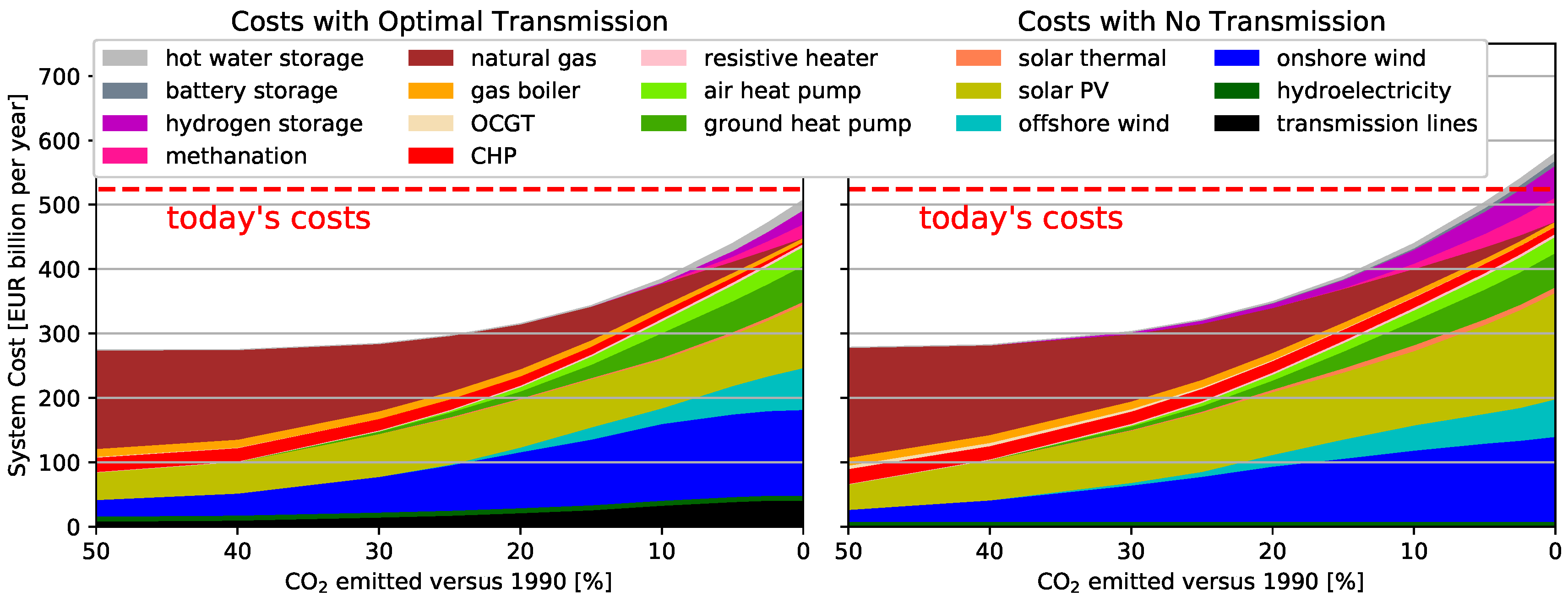
3.1. Total System Costs

In Figure 3, the composition of the total system costs, including transmission, generation, and storage, is shown as the CO${}_2$ limit is made successively stricter, with cost-optimal cross-border transmission (left) and no cross-border transmission (right). The case of no cross-border transmission is provided as a reference point for the many single-country studies in the literature [10,11,12,13,14,15,16,17,18] that do not consider cross-border transfers, and to quantify the full benefit of interconnection. Interconnection was shown, in many studies, to help to balance variable renewable energy sources, particularly wind, and to reduce the costs of carbon dioxide mitigation [2,4,6,43,44,45,46,47,48,49,50,51].

In both systems, the CO${}_2$ constraint is non-binding, down to 50% of the 1990 emissions. In other words, the greenfield cost optima with no CO${}_2$ constraint or pricing already result in a large CO${}_2$ reduction, largely due to new installations of CHPs fired by natural gas and around a 50% share of renewables in the electricity supply. If there were other cheaper, but more CO${}_2$ intensive, generators in the model, such as coal, this minimum would be at a higher level of CO${}_2$ emissions. For comparison, the 2016 emissions in the energy sectors considered here were 14.2% below their 1990 level.

The cost of today’s system is estimated to be 524 billion euros per year, making the greenfield, unconstrained cost-optimum 48% cheaper than the current system. Today’s costs are hard to gauge precisely, because of legacy investments over decades, but for this estimate we have assumed an average cost of electricity generation (including investment) of 70 €/MWh${}_{\mathrm{el}}$, 8 €/MWh${}_{\mathrm{th}}$ for solid fuels, 47 €/MWh${}_{\mathrm{th}}$ for oil, and 22 €/MWh${}_{\mathrm{th}}$ for gas, and assume that the entire non-electric heat load is met by fossil fuel boilers priced like gas boilers, which are dimensioned to meet the peak thermal load in each country. With these assumptions and energy consumption figures from the Eurostat energy balances for 2011 [52], the costs are 221 billion €/a for electricity generation (this agrees with the estimate based on price tariff statistics in [7], which excludes network costs and taxes), 3 billion €/a for cross-border transmission, 167 billion €/a for land transport fuels, 98 billion €/a for heating fuels, and 35 billion €/a for the boilers; resulting in a grand total of 524 billion €/a.

As the CO${}_2$ limit is reduced below 50% and down to zero, costs rise by 108% with no transmission, and by 85% with optimal transmission. With zero direct CO${}_2$ emissions and optimal transmission, system costs are 3% below today’s costs, for the 2030 cost projections used here. Higher costs at lower emissions are driven by the need to defossilise heating, which is supplied by a combination of heat pumps and synthetic methane to bridge multi-day periods with low wind and solar energy. Bioenergy could also be used to bridge these periods and, thus, lower costs. However, as we discuss in Section 4, there is uncertainty regarding the sustainability of its widespread use and also strong competition from aviation, shipping, production of plastics, and other non-electric industrial demand for limited sustainable bioenergy resources.

The cost rise is more pronounced with no transmission, since variable renewables cannot be balanced between countries, but must be balanced for each country, in a self-sufficient manner, by using storage. In the case of optimal transmission, despite the extra costs of the transmission infrastructure, the costs of the total zero-CO${}_2$ system are 13% lower than the no-transmission case. The optimal amount of transmission grows by a factor of 5 as the CO${}_2$ limit is reduced, reflecting how the benefit of transmission increases as more variable renewables enter the electricity system. Transmission helps to balance the variability of renewables over space, particularly for wind, because wind has a synoptic-scale correlation length of 400–600 km [53], which is smaller than the size of the continent. At zero direct carbon dioxide emissions, the total volume of cross-border transmission (the sum of length times capacity for each line, where the length is the distance between the country centres) is 382 TWkm, which is over 12 times today’s volume of 31 TWkm. Given the current public acceptance issues for overhead transmission, some of these transmission projects would have to be traded against the slightly higher costs of scenarios with less cross-border transmission.

For the rest of this article, we focus on the results from the case with optimal transmission.

From the map of investments, in Figure 1, it can be seen that the optimal transmission network is particularly strong between northern countries, where it can balance their plentiful wind resources. Power-to-gas investment is strongest in the peripheral countries, where it is not cost-optimal to build cross-border grid capacity to absorb all excess renewable generation. In central countries, such as Germany, there is so much grid capacity that power-to-gas is not cost effective, at least for the 2030 cost projections used here.

In Figure 4, the total cost behaviour is reflected in the shadow price ${\mu }_{{\mathrm{CO}}_2}$ of the CO${}_2$ constraint (Equation (2)) as the CO${}_2$ limit is tightened. The CO${}_2$ price rises from zero at the non-binding 50% CO${}_2$ reduction, to around 500 €/tCO${}_2$ once all CO${}_2$ is eliminated from the model. As pointed out in [29], this high price is a direct reflection of the difference between the cost of natural gas (21.6 €/MWh${}_{\mathrm{th}}$) and the high price of synthetic methane in the model (113.7 €/MWh${}_{\mathrm{th}}$), which is needed for low-fossil heating. It is significantly higher than the January 2019 price of 20–25 €/tCO${}_2$ in the European Emissions Trading System (ETS), which covers power generation, some industrial sectors, and aviation, amounting to around half of all European CO${}_2$ emissions. The price is so high that it may be more cost-effective to eliminate CO${}_2$ in the other sectors not covered in the model, such as aviation, shipping, industry, or, indeed, by capture directly from the air.

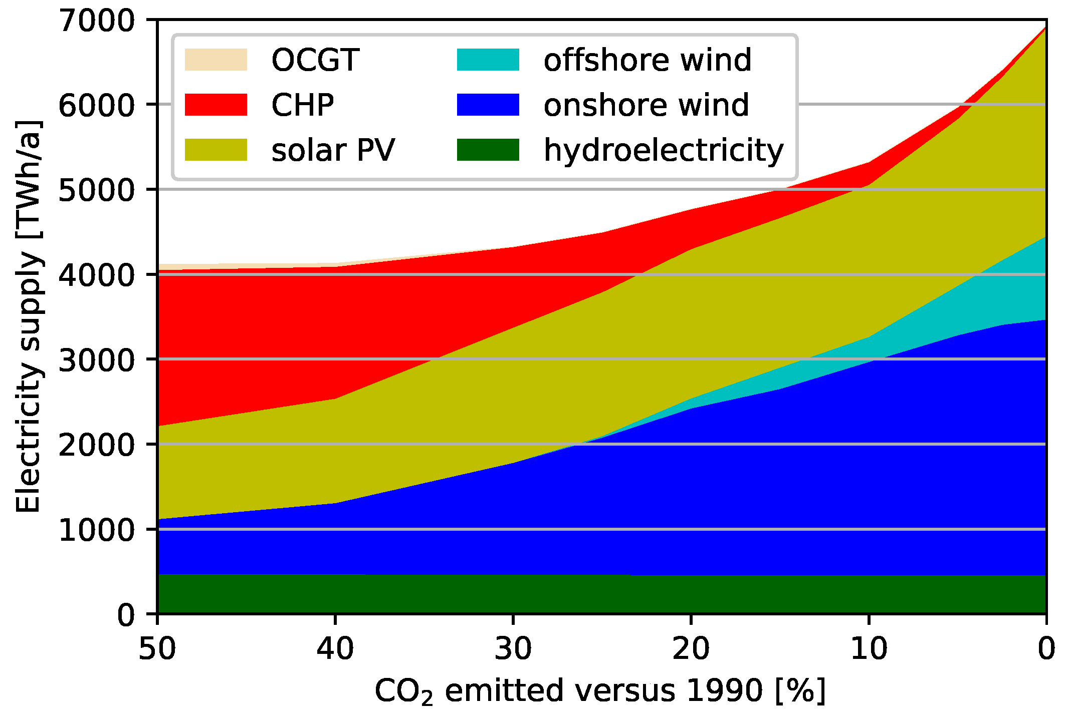
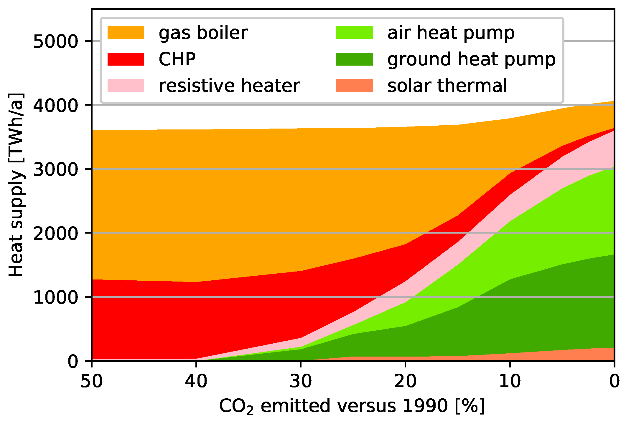
3.2. Defossilisation of Sectors

Next, we examine how the different sectors are defossilised. Because the model includes only the transport fuel costs and not the capital costs of vehicles, transport is electrified immediately as the electricity consumed for each kilometre travelled is less costly than petrol or diesel. The fossil-share for transport, then, reflects the fossil-share in electricity. The projected capital costs for electric vehicles in 2030 are comparable or lower than those for internal combustion engine vehicles [38], so the inclusion of these costs would not alter the early electrification of transport. Turning to electricity and heating, the picture is more complicated, as can be seen from the fossil fuel shares in Figure 5, the electricity supply in Figure 6, and the water and space heating supply in Figure 7. Electricity and electrified transport are defossilised swiftly, whereas heating only begins to be defossilised in earnest below 30% total CO${}_2$ emissions, with the majority of the reduction coming at the end below 20%. This can also be seen in the total investments in Figure 3.

The electricity supply in Figure 6 sees a rapid increase in wind and solar installations, with the remaining electricity demand being supplied by existing hydroelectric plants and combined heat and power (CHP) stations. The renewable energy share increases (Figure 5) at the same time as total electricity demand increases (Figure 6). With zero net emissions, the total electricity demand is more than double the 2011 total of 3153 TWh${}_{\mathrm{el}}$/a. This increase is due to the electrification of transport and heating, as well as conversion losses in the power-to-gas and other storage units.

In the heating sector (Figure 7), when the CO${}_2$ constraint is non-binding, heating is provided cheaply by natural gas in either gas boilers or CHPs. Heating is defossilised mostly by heat pumps, which drive up costs because, as well as the units themselves, they also require additional electricity generation capacity. Smaller contributions are made from resistive heaters and solar thermal collectors, while some gas boilers remain at the end to provide backup heat with synthetic methane. The overall heat demand rises slightly towards zero emissions, because of conversion losses in long-term thermal storage facilities in district heating networks.

It was identified, in [29], that one of the hardest aspects of the defossilisation of heating is the long winter cold spells with low generation from wind and solar, high heating demand, and lower heat pump coefficients of performance. Heating in these periods can be achieved by producing synthetic methane or by using long-term thermal energy storage, but particularly the former drives up system costs significantly. This effect can be seen in the rise of system costs, in Figure 3, as the last CO${}_2$ is removed from the system using the power-to-gas facilities.

The expense of fully defossilising space and water heating was also confirmed in [54], which showed that cheap and abundant renewable energy is not sufficient to incentivise the full defossilisation of heating. CO${}_2$ prices are also required to narrow the cost differential between gas and low-carbon options.

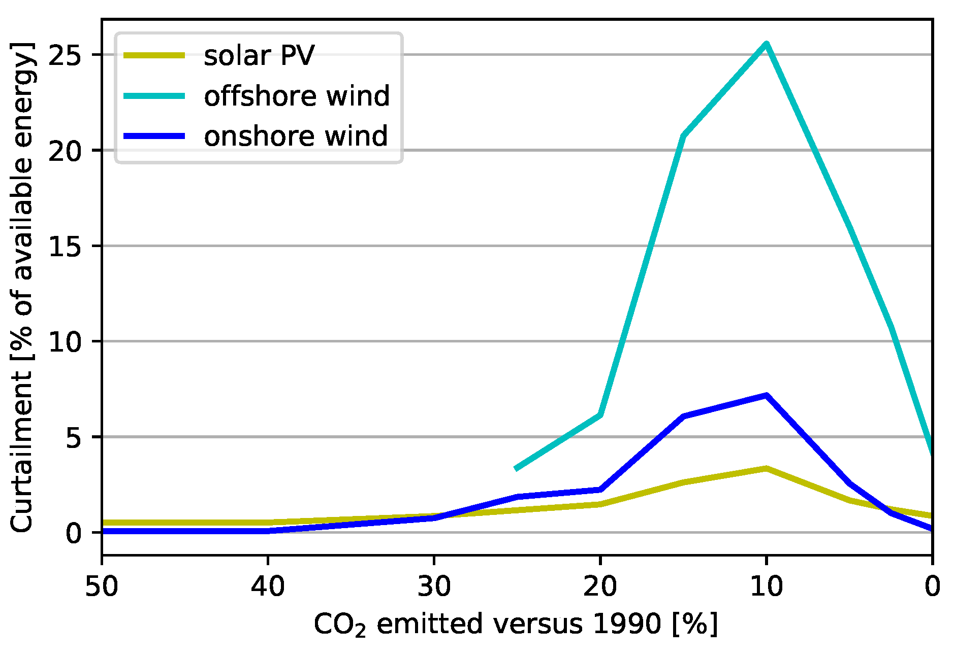
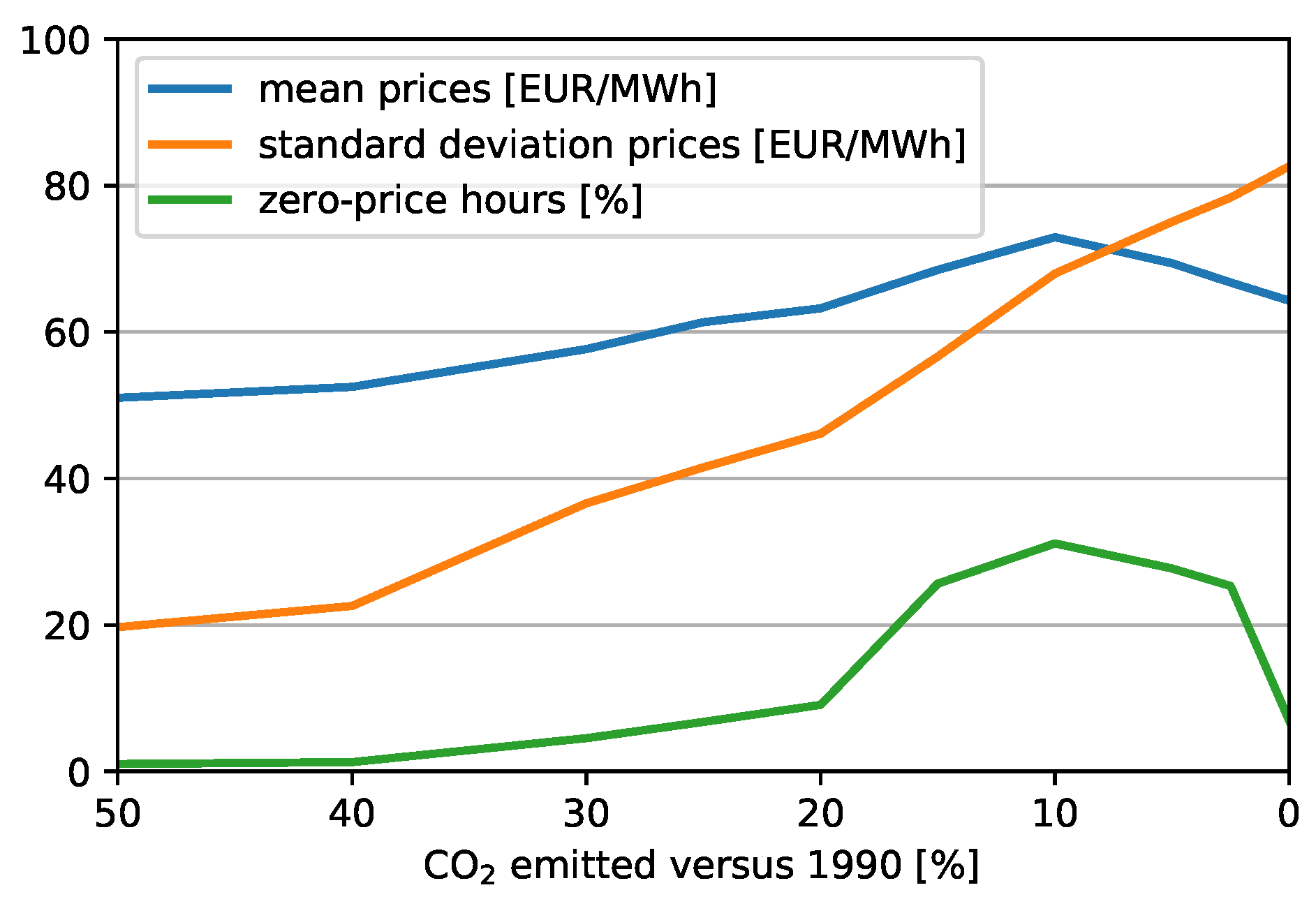
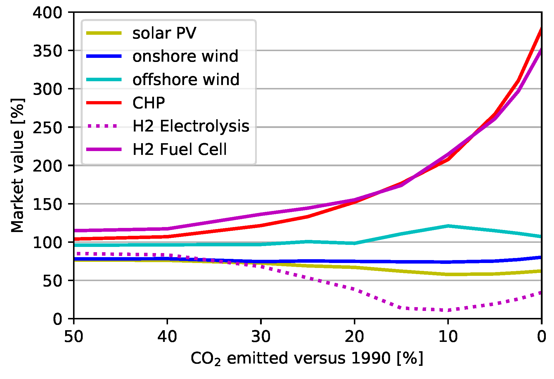
3.3. Metrics for VRE Integration

In this section, the curtailment, market prices, and market values of the different technologies are considered.

Power-to-gas is forced into the system primarily by the need for synthetic fuels in the heating sector during cold spells. However, its introduction has big effects on the operation of other system components and market behaviour. In Figure 8, the effect on curtailment is plotted. As CO${}_2$ is reduced below 20%, curtailment initially rises, reaching a peak of 26% of offshore wind, 7% of onshore wind, and 3% of solar available energy, at a level of 10% CO${}_2$. This reflects the strong seasonal peaking of the heating demand, which is hard to match with the output of solar and even with wind, which also peaks in the winter. Below 10% CO${}_2$, it becomes cost-optimal to invest in power-to-gas. This means that any excess renewable energy can can be converted into synthetic fuels, removing almost all the curtailment when direct carbon dioxide emissions reach zero. Curtailment is worse for offshore wind than onshore or solar as, during times of excess, the dispatch rules were chosen so that offshore wind is curtailed first, then onshore wind, then solar. Offshore wind is not plotted above 25% carbon dioxide reduction, because its feed-in was negligible for these values.

A similar turning point can be seen in the electricity price statistics, plotted in Figure 9. For these statistics, all averages are weighted by the electric load, which includes electric vehicles, heat pumps, resistive heaters, and storage units in charging mode. The percentage of hours with zero marginal prices in the model drops from a peak of 31% of hours at 10% CO${}_2$, to just 6.9% of hours at 0% CO${}_2$. With power-to-gas, it becomes worthwhile to put renewables to economic use in almost every hour, and only in a small fraction of hours is there an excess of renewable energy. Figure 9 also shows rising market prices until 10% CO${}_2$, reflecting the increase in total system costs, at which point the introduction of large flexible demand from electrolysers allows low-price hours to be better used. This drives down average prices since, here, the prices are weighted by the volume of the electrical load in each hour. The simple time-weighted average electricity price increases monotonically to 78 €/MWh${}_{\mathrm{el}}$ as emissions tend to zero. Prices for heating, hydrogen, and methane also increase monotonically. The rising standard deviation in the electricity prices reflects rising volatility from the increasing shares of variable wind and solar generation.

The turning point is, again, reflected in the market values of the different technologies connected to the electricity system, as shown in Figure 10. Here, we define the market value as the average price of each unit of electricity consumed or produced by each technology, relative to the average load-weighted price; that is,

$${\mathrm{MV}}_s=\frac{{\sum }_{n,t}{\lambda }_{n,t}{g}_{n,s,t}}{{\sum }_{n,t}{g}_{n,s,t}}{\left(\frac{{\sum }_{n,t}{\lambda }_{n,t}{d}_{n,t}}{{\sum }_{n,t}{d}_{n,t}}\right)}^{-1},$$

(3)

where ${\lambda }_{n,t}$ is the locational marginal price from Equation (1), $g_{n,s,t}$ is the generator dispatch, and the demand $d_{n,t}$ includes electric vehicles, heat pumps, resistive heaters, and storage units in charging mode. In the language of [9], ${\mathrm{MV}}_s$ is the long-term value factor. The market value gives a useful indication of the value of each technology to the system.

In general, it is expected, from other studies [8,9], that the market value of variable renewable generators, such as wind and solar, should reduce with higher penetration, as they decrease the market prices in exactly the hours when they produce at high volume, thanks to the merit order effect. Down to 10% CO${}_2$, the relative market values do indeed diverge, with onshore wind and solar receiving low market values, while less-variable offshore wind reaches 121% market value and storage units achieve ever-stronger price arbitrage. However, below 10% CO${}_2$, the market values of the variable generation technologies begin to converge to 100% again, as increased flexibility, in particular from power-to-gas, creates a market for wind and solar power. Below 10%, electrolysers pay increasingly higher prices for electricity as the demand for hydrogen increases, reaching an average price of 22 €/MWh${}_{\mathrm{el}}$ paid for electricity by electrolysers at zero CO${}_2$ emissions (this price is obtained by multiplying the value factor 34% from Figure 10 with the average price 64 €/MWh${}_{\mathrm{el}}$ from Figure 9). This results in an average marginal price of hydrogen of 49 €/MWh${}_{\mathrm{th}}$ (27.5 €/MWh${}_{\mathrm{th}}$ for the electricity and the rest for investments in electrolysers and hydrogen storage).

It can be concluded that in a highly-integrated sector-coupled low-carbon system, the market values of wind and solar do not decline as precipitously as has been observed at lower renewable penetrations in electricity-only models [9]. Theoretically, this is inevitable: Given that all actors make back their costs from market prices in a long-term equilibrium (like this model), and that VRE make up the majority of the total system costs, VRE cost recovery constitutes a large share of the market prices.

The increasing interaction between electricity market prices and the production and consumption of synthetic gas is also strongly reflected in the time series; see Figure 11. The gas dispatch and electricity price are strongly correlated, with a Pearson correlation coefficient of 0.82 with zero CO${}_2$ emissions. This correlation is stronger than the correlation of the prices with the residual load ($-0.30$) or variable renewable generation ($-0.33$). When renewables are abundant and other demand is low (particularly, in the summer), prices are low, and so a lot of synthetic gas is produced; the methanation units achieve an average of 4953 full load hours, thus enabling them to recover their high capital costs. When renewables are scarce and demand is high, particularly in the winter, gas is consumed in electricity and heating as a backup.

4. Limitations of this Study

An extensive discussion of the limitations of the model PyPSA-Eur-Sec-30 can be found in the paper that introduced the model [29], while a sensitivity analysis on many of the costs and other assumptions in the electricity sector was carried out in [55]. Here, aspects are highlighted that particularly impact the results discussed in this paper.

One of the primary limitations of this study is the exclusion of biomass as a technology option. Biomass was excluded, partly because of the large uncertainties surrounding the sustainability of its widespread use [56], and partly because there is likely to be intense competition for limited sustainable biomass potentials from the other hard-to-defossilise sectors that are not included in this model: Plastics production, other non-electric industrial demand, shipping, and aviation. Biomass could help to alleviate the cost peak in Figure 3, by reducing the need for synthetic gas. Biofuels could act as a bridge for existing internal combustion engine vehicles before electric vehicles become prevalent, although, in the long-term, their use should probably be restricted to hard-to-electrify sectors, such as aviation [57]. Bioenergy with carbon capture and sequestration (BECCS) may also play an important role in long-term mitigation scenarios by providing negative emissions, although there is some scepticism about the widespread use of this technology in integrated assessment models [58,59,60,61]. Given that sustainable biomass resources are limited [62], once the other sectors are included, the demand for synthetic fuels will remain high, so that the effects seen in this paper are likely to remain. This has been confirmed in an upcoming study by some of the authors.

Including the full industrial sector would also allow the model to consider the indirect emissions during production of energy infrastructure assets (only direct emissions have been included here).

Given the focus in this paper on a high share of renewables, which is also the policy goal of many EU member states, nuclear and fossil generation with carbon capture and sequestration (CCS) were not considered. The time-weighted mean electricity price with zero emission was 78 €/MWh${}_{\mathrm{el}}$, which is the price with which nuclear or fossil with CCS would have to compete. Recent nuclear projects in Europe have not been able to attain this price level. CCS may still be necessary in the future for the net negative emissions that are required in many scenarios that meet the Paris Agreement targets [32].

Other uncertainties concern the availability and costs of relatively new technologies, such as battery electric vehicles with vehicle-to-grid functionality and power-to-gas infrastructure; the sensitivity of the results to these assumptions was examined in [29,55] and found to be below 10%. As can be seen from their shares in the cost structure in Figure 3, the primary sensitivities are, in fact, to the costs of wind, solar, and heat pumps and, of course, to the discount rate. Even doubling the costs of power-to-gas infrastructure has only a limited effect on the total costs. The solar cost reductions for 2030 assumed here are ambitious, but are in line with recent cost declines. A full range of PV costs, going all the way down to zero, were examined in [55], and, although more PV investment is seen with lower costs, in Europe the PV penetration is limited by a generation pattern that is anti-correlated with the seasonal variations in demand. If the cost projections for electric vehicles used here prove to be too ambitious, this may delay the electrification of land transport.

Further modelling limitations include the restriction to a single representative historical year and the assumption of perfect foresight and of perfect markets; these limitations are driven by computational restrictions. Distribution grid reinforcement was not considered, since it does not represent a public acceptance problem, and because the costs of reinforcement are likely to be low compared to total system costs [7].

5. Conclusions

In this paper, we have studied the changes in energy system properties as the constraint on allowed direct CO${}_2$ emissions is varied, in a sector-coupled model covering European electricity, heating, and land transport demand. A reduction in CO${}_2$ emissions of 50%, compared to 1990 levels, for the considered low-carbon technologies is cost-effective, regardless of the level of transmission expansion, thanks to increasing shares of cheap wind and solar electricity and the electrification of land transport. Below this level, costs rise as carbon dioxide is initially pushed out of the system by heat pumps and, finally, by the synthetic fuels that are necessary to bridge long cold spells with low wind and sun. However, even with zero direct CO${}_2$ emissions, the total system costs are comparable to the costs of today’s energy system, when using cost projections for 2030.

The introduction of power-to-gas, driven by these cold spells when cheap low-emission electricity is scarce, alters market dynamics because of the ease of the long-term storage of gas. This results in fewer hours of zero prices, substantially less curtailment, and a re-convergence of the market values of variable renewable generators towards the average market price.

While some synthetic gas could be replaced by bioenergy in the model, either in the form of solid biomass or biogas upgraded to biomethane, it should also be borne in mind that scarce sustainable bioenergy resources will also be required in other sectors which are harder to electrify, such as aviation, shipping, plastics production, and other non-electric industrial demand. Exploring these trade-offs in a high resolution model is an interesting topic for future research.

While model limitations should be borne in mind, several relevant policy measures can be deduced from the results: Increasing low-emission technologies in electricity generation is a priority, particularly given that defossilisation strategies in other sectors rely on electrification; reducing emissions in space and water heating is more expensive and sees investment accelerate towards the end of the energy transition; CO${}_2$ prices (or equivalent second-best measures, like mandates for district heating or heat pumps) will be required across all sectors and at levels much higher than seen today in the European Emissions Trading System; power-to-gas is an important part of guaranteeing system security during cold winter wind lulls, and so investment in research, development, and deployment should be increased to guarantee that power-to-gas can scale up in time; zero-emission systems can be cost-effective, even before accounting for the health and environmental benefits, so expense is not a limitation for the energy transition; it may be cost-effective to go further than the EU’s current 40% greenhouse gas reduction target for 2030 and aim for zero net-emissions in 2050, pending further investigations of the integration of industrial, shipping, and aviation demand.

References

1. Czisch, G. Szenarien Zur Zukünftigen Stromversorgung. Ph.D. Thesis, Universität Kassel, Kassel, Germany, 2005. [Google Scholar]
2. Scholz, Y. Renewable Energy Based Electricity Supply at Low Costs—Development of the REMix Model and Application for Europe. Ph.D. Thesis, Universität Stuttgart, Stuttgart, Germany, 2012. [Google Scholar]
3. Gils, H.C.; Scholz, Y.; Pregger, T.; de Tena, D.L.; Heide, D. Integrated modelling of variable renewable energy-based power supply in Europe. Energy 2017, 123, 173–188. [Google Scholar] [CrossRef]
4. Schlachtberger, D.; Brown, T.; Schramm, S.; Greiner, M. The benefits of cooperation in a highly renewable European electricity network. Energy 2017, 134, 469–481. [Google Scholar] [CrossRef]
5. Reichenberg, L.; Hedenus, F.; Odenberger, M.; Johnsson, F. The marginal system LCOE of variable renewables—Evaluating high penetration levels of wind and solar in Europe. Energy 2018, 152, 914–924. [Google Scholar] [CrossRef]
6. Child, M.; Kemfert, C.; Bogdanov, D.; Breyer, C. Flexible electricity generation, grid exchange and storage for the transition to a 100% renewable energy system in Europe. Renew. Energy 2019, 139, 80–101. [Google Scholar] [CrossRef]
7. Brown, T.; Bischof-Niemz, T.; Blok, K.; Breyer, C.; Lund, H.; Mathiesen, B. Response to ‘Burden of proof: A comprehensive review of the feasibility of 100% renewable-electricity systems’. Renew. Sustain. Energy Rev. 2018, 92, 834–847. [Google Scholar] [CrossRef]
8. Joskow, P.L. Comparing the costs of intermittent and dispatchable electricity generating technologies. Am. Econ. Rev. 2011, 101, 238–241. [Google Scholar] [CrossRef]
9. Hirth, L. The market value of variable renewables: The effect of solar wind power variability on their relative price. Energy Econ. 2013, 38, 218–236. [Google Scholar] [CrossRef]
10. Henning, H.M.; Palzer, A. A comprehensive model for the German electricity and heat sector in a future energy system with a dominant contribution from renewable energy technologies—Part I: Methodology. Renew. Sustain. Energy Rev. 2014, 30, 1003–1018. [Google Scholar] [CrossRef]
11. Palzer, A.; Henning, H.M. A comprehensive model for the German electricity and heat sector in a future energy system with a dominant contribution from renewable energy technologies—Part II: Results. Renew. Sustain. Energy Rev. 2014, 30, 1019–1034. [Google Scholar] [CrossRef]
12. Gerhardt, N.; Scholz, A.; Sandau, F.; Hahn, H. Interaktion EE-Strom, Wärme und Verkehr; Technical Report; Fraunhofer IWES: Kassel, Germany, 2015. [Google Scholar]
13. Quaschning, V. Sektorkopplung Durch die Energiewende; Technical Report; HTW Berlin: Berlin, Germany, 2016. [Google Scholar]
14. Lund, H.; Mathiesen, B. Energy system analysis of 100% renewable energy systems—The case of Denmark in years 2030 and 2050. Energy 2009, 34, 524–531. [Google Scholar] [CrossRef]
15. Mathiesen, B.V.; Lund, H.; Conolly, D.; Wenzel, H.; Østergaard, P.; Möller, B.; Nielsen, S.; Ridjan, I.; Karnøe, P.; Sperling, K.; et al. Smart Energy Systems for coherent 100% renewable energy and transport solutions. Appl. Energy 2015, 145, 139–154. [Google Scholar] [CrossRef]
16. Lund, H.; Andersen, A.N.; Østergaard, P.A.; Mathiesen, B.V.; Connolly, D. From electricity smart grids to smart energy systems—A market operation based approach and understanding. Energy 2012, 42, 96–102. [Google Scholar] [CrossRef]
17. Connolly, D.; Lund, H.; Mathiesen, B.; Leahy, M. The first step towards a 100% renewable energy-system for Ireland. Appl. Energy 2011, 88, 502–507. [Google Scholar] [CrossRef]
18. Deane, J.; Chiodi, A.; Gargiulo, M.; Gallachoir, B.P.O. Soft-linking of a power systems model to an energy systems model. Energy 2012, 42, 303–312. [Google Scholar] [CrossRef]
19. Connolly, D.; Lund, H.; Mathiesen, B. Smart Energy Europe: The technical and economic impact of one potential 100% renewable energy scenario for the European Union. Renew. Sustain. Energy Rev. 2016, 60, 1634–1653. [Google Scholar] [CrossRef]
20. The PRIMES Model; Technical Report; NTUA: Athens, Greece, 2009.
21. Leimbach, M.; Bauer, N.; Baumstark, L.; Luken, M.; Edenhofer, O. Technological change and international trade—Insights from REMIND-R. Energy J. 2010, 31. [Google Scholar] [CrossRef]
22. Capros, P.; Paroussos, L.; Fragkos, P.; Tsani, S.; Boitier, B.; Wagner, F.; Busch, S.; Resch, G.; Blesl, M.; Bollen, J. European decarbonisation pathways under alternative technological and policy choices: A multi-model analysis. Energy Strategy Rev. 2014, 2, 231–245. [Google Scholar] [CrossRef]
23. Hagspiel, S.; Jägemann, C.; Lindenburger, D.; Brown, T.; Cherevatskiy, S.; Tröster, E. Cost-optimal power system extension under flow-based market coupling. Energy 2014, 66, 654–666. [Google Scholar] [CrossRef]
24. Simoes, S.; Nijs, W.; Ruiz, P.; Sgobbi, A.; Thiel, C. Comparing policy routes for low-carbon power technology deployment in EU—An energy system analysis. Energy Policy 2017, 101, 353–365. [Google Scholar] [CrossRef]
25. Löffler, K.; Hainsch, K.; Burandt, T.; Oei, P.Y.; Kemfert, C.; von Hirschhausen, C. Designing a model for the global energy system—GENeSYS-MOD: An application of the open-source energy modeling system (OSeMOSYS). Energies 2017, 10, 1468. [Google Scholar] [CrossRef]
26. Blanco, H.; Nijs, W.; Ruf, J.; Faaij, A. Potential for hydrogen and power-to-liquid in a low-carbon EU energy system using cost optimization. Appl. Energy 2018, 232, 617–639. [Google Scholar] [CrossRef]
27. Ludig, S.; Haller, M.; Schmid, E.; Bauer, N. Fluctuating renewables in a long-term climate change mitigation strategy. Energy 2011, 36, 6674–6685. [Google Scholar] [CrossRef]
28. Kotzur, L.; Markewitz, P.; Robinius, M.; Stolten, D. Impact of different time series aggregation methods on optimal energy system design. Renew. Energy 2018, 117, 474–487. [Google Scholar] [CrossRef]
29. Brown, T.; Schlachtberger, D.; Kies, A.; Greiner, M. Synergies of sector coupling and transmission extension in a cost-optimised, highly renewable European energy system. Energy 2018, 160, 720–730. [Google Scholar] [CrossRef]
30. Millar, R.J.; Fuglestvedt, J.S.; Friedlingstein, P.; Rogelj, J.; Grubb, M.J.; Matthews, H.D.; Skeie, R.B.; Forster, P.M.; Frame, D.J.; Allen, M.R. Emission budgets and pathways consistent with limiting warming to 1.5 °C. Nat. Geosci. 2017, 10, 741. [Google Scholar] [CrossRef]
31. European Commission. Energy Roadmap 2050—COM(2011) 885/2; European Commission: Brussel, Belgium, 2011. [Google Scholar]
32. UNFCCC. Adoption of the Paris Agreement. Report No. FCCC/CP/2015/L.9/Rev.1. 2015. Available online: http://unfccc.int/resource/docs/2015/cop21/eng/l09r01.pdf (accessed on 21 January 2019).
33. European Council. Presidency Conclusions—Brussels, 29/30 October 2009; Council of thr European Union: Brussels, Belgium, 2009. [Google Scholar]
34. European Commission. A Clean Planet for All—COM(2018) 773; European Commission: Brussel, Belgium, 2018. [Google Scholar]
35. National Emissions Reported to the UNFCCC and to the EU Greenhouse Gas Monitoring Mechanism; Technical report; European Environmental Agency: Copenhagen, Denmark, 2018.
36. Rogelj, J.; Popp, A.; Calvin, K.V.; Luderer, G.; Emmerling, J.; Gernaat, D.; Fujimori, S.; Strefler, J.; Hasegawa, T.; Marangoni, G.; et al. Scenarios towards limiting global mean temperature increase below 1.5 °C. Nat. Clim. Chang. 2018, 8, 325–332. [Google Scholar] [CrossRef]
37. Persson, U.; Werner, S. Heat distribution and the future competitiveness of district heating. Appl. Energy 2011, 88, 568–576. [Google Scholar] [CrossRef]
38. Electric Vehicle Outlook 2017; Technical report; Bloomberg New Energy Finance: New York City, NY, USA, 2017.
39. ODYSSEE Database on Energy Efficiency Data & Indicators; Technical report; Enerdata: Grenoble, France, 2016.
40. Brown, T.; Hörsch, J.; Schlachtberger, D. PyPSA: Python for power system analysis. J. Open Res. Softw. 2018, 6. [Google Scholar] [CrossRef]
41. Brown, T.; Schlachtberger, D. Supplementary Data: Code, Input Data and Result Summaries: Synergies of sector coupling and transmission extension in a cost-optimised, highly renewable European energy system (Version v0.1.0) [Data set]. Zenodo 2018. [Google Scholar] [CrossRef]
42. Brown, T.; Schlachtberger, D. Supplementary Data: Full Results: Synergies of sector coupling and transmission extension in a cost-optimised, highly renewable European energy system (Version v0.1.0) [Data set]. Zenodo 2018. [Google Scholar] [CrossRef]
43. Bahn, O.; Haurie, A.; Kypreos, S.; Vial, J. Advanced mathematical programming modeling to assess the benefits from international CO2 abatement cooperation. Environ. Model. Assess. 1998, 3, 107–115. [Google Scholar] [CrossRef]
44. Unger, T.; Ekvall, T. Benefits from increased cooperation and energy trade under CO2 commitments— The Nordic case. Clim. Policy 2003, 3, 279–294. [Google Scholar] [CrossRef]
45. Czisch, G. Szenarien zur Zukünftigen Stromversorgung: Kostenoptimierte Variationen zur Versorgung Europas und Seiner Nachbarn mit Strom aus Erneuerbaren Energien. Ph.D. Thesis, Universität Kassel, Kassel, Germany, 2005. [Google Scholar]
46. Schaber, K.; Steinke, F.; Hamacher, T. Transmission grid extensions for the integration of variable renewable energies in Europe: Who benefits where? Energy Policy 2012, 43, 123–135. [Google Scholar] [CrossRef]
47. Schaber, K.; Steinke, F.; Mühlich, P.; Hamacher, T. Parametric study of variable renewable energy integration in Europe: Advantages and costs of transmission grid extensions. Energy Policy 2012, 42, 498–508. [Google Scholar] [CrossRef]
48. Rodriguez, R.; Becker, S.; Andresen, G.; Heide, D.; Greiner, M. Transmission needs across a fully renewable European power system. Renew. Energy 2014, 63, 467–476. [Google Scholar] [CrossRef]
49. MacDonald, A.E.; Clack, C.T.M.; Alexander, A.; Dunbar, A.; Wilczak, J.; Xie, Y. Future cost-competitive electricity systems and their impact on US CO2 emissions. Nat. Clim. Chang. 2017, 6, 526–531. [Google Scholar] [CrossRef]
50. Eriksen, E.H.; Schwenk-Nebbe, L.J.; Tranberg, B.; Brown, T.; Greiner, M. Optimal heterogeneity in a simplified highly renewable European electricity system. Energy 2017, 133, 913–928. [Google Scholar] [CrossRef]
51. Galán-Martín, A.; Pozo, C.; Azapagic, A.; Grossmann, I.E.; Mac Dowell, N.; Guillén-Gosálbez, G. Time for global action: An optimised cooperative approach towards effective climate change mitigation. Energy Environ. Sci. 2018, 11, 572–581. [Google Scholar] [CrossRef]
52. Energy Balances 1900–2014; Technical Report; Eurostat: Luxembourg, 2016.
53. Kiss, P.; Jánosi, I.M. Limitations of wind power availability over Europe: A conceptual study. Nonlinear Process. Geophys. 2008, 15, 803–813. [Google Scholar] [CrossRef]
54. Zhu, K.; Victoria, M.; Brown, T.; Andresen, G.; Greiner, M. Impact of CO2 prices on the design of a highly decarbonised coupled electricity and heating system in Europe. Appl. Energy 2019, 236, 622–634. [Google Scholar] [CrossRef]
55. Schlachtberger, D.; Brown, T.; Schäfer, M.; Schramm, S.; Greiner, M. Cost optimal scenarios of a future highly renewable European electricity system: Exploring the influence of weather data, cost parameters and policy constraints. Energy 2018, 163, 100–114. [Google Scholar] [CrossRef]
56. Creutzig, F.; Ravindranath, N.H.; Berndes, G.; Bolwig, S.; Bright, R.; Cherubini, F.; Chum, H.; Corbera, E.; Delucchi, M.; Faaij, A.; et al. Bioenergy and climate change mitigation: An assessment. GCB Bioenergy 2015, 7, 916–944. [Google Scholar] [CrossRef]
57. Connolly, D.; Mathiesen, B.; Ridjan, I. A comparison between renewable transport fuels that can supplement or replace biofuels in a 100% renewable energy system. Energy 2014, 73, 110–125. [Google Scholar] [CrossRef]
58. Fuss, S.; Canadell, J.G.; Peters, G.P.; Tavoni, M.; Andrew, R.M.; Ciais, P.; Jackson, R.B.; Jones, C.D.; Kraxner, F.; Nakicenovic, N.; et al. Betting on negative emissions. Nat. Clim. Chang. 2014, 4, 850–853. [Google Scholar] [CrossRef]
59. Smith, P.; Davis, S.J.; Creutzig, F.; Fuss, S.; Minx, J.; Gabrielle, B.; Kato, E.; Jackson, R.B.; Cowie, A.; Kriegler, E.; et al. Biophysical and economic limits to negative CO2 emissions. Nat. Clim. Chang. 2015, 6. [Google Scholar] [CrossRef]
60. Anderson, K.; Peters, G. The trouble with negative emissions. Science 2016, 354, 182–183. [Google Scholar] [CrossRef]
61. Vaughan, N.E.; Gough, C. Expert assessment concludes negative emissions scenarios may not deliver. Environ. Res. Lett. 2016, 11, 095003. [Google Scholar] [CrossRef]
62. Ruiz, P.; Sgobbi, A.; Nijs, W.; Thiel, C.; Longa, F.; Kober, T. The JRC-EU-TIMES Model: Bioenergy Potentials; Technical Report; JRC: Petten, The Netherlands, 2015. [Google Scholar] [CrossRef]
Figure 1. Costs by country with zero CO 2 emissions and optimal transmission. The colour assignments follow Figure 3.
Energies 12 01032 g001
Figure 2. Energy flow at a single node. In this model, a node represents a whole European country. Within each node, there is a bus (thick horizontal line) for each energy carrier (electric, transport, heat, hydrogen, and methane), to which different loads (triangles), energy sources (circles), storage units (rectangles), and converters (lines connecting buses) are attached. The lines with arrows show the direction of energy transfer (Source: [29]).
Energies 12 01032 g002
Figure 3. System costs for electricity, land transport, and space and water heating in Europe with a changing CO 2 limit, assuming the 2030 cost projections from Table 1. Left is the case with cost-optimal transmission, right is with no transmission. Estimated costs for today’s system are marked with a red dashed line.
Energies 12 01032 g003
Figure 4. CO 2 shadow price in the model as CO 2 emissions are restricted in the case of cost-optimal cross-border transmission.
Energies 12 01032 g004
Figure 5. Share of fossil fuel energy provision in electricity, electrified transport, and heat.
Energies 12 01032 g005
Figure 6. Breakdown of electricity supply by technology.
Energies 12 01032 g006
Figure 7. Breakdown of space and water heating supply by technology.
Energies 12 01032 g007
Figure 8. Curtailed variable renewable energy, as a percentage of the available energy.
Energies 12 01032 g008
Figure 9. Load-weighted statistics of electricity prices.
Energies 12 01032 g009
Figure 10. Market values relative to the average load-weighted price.
Energies 12 01032 g010
Figure 11. Zero CO 2 scenario: Methane dispatch (positive when synthetic methane is consumed, negative when produced by methanation) versus average electricity prices.
Energies 12 01032 g011