Parameter-Free Fault Location Algorithm for Distribution Network T-Type Transmission Lines

Abstract

T-type transmission lines have been increasingly used in distribution networks because of the distributed generation integration, but inaccurate line parameters will cause significant error in the results of most existing fault location algorithms for this kind of line. In order to improve the precision, this paper proposes a new fault location algorithm taking line parameters as unknowns. The fault is assumed to occur on each section, and corresponding ranging equations can be built based on one set of three-terminal post-fault synchronous measurements, without using line parameters as inputs. Then, more sets of measurements are utilized to increase the redundancy of equations to resist the influence of data error. The reliable trust-region algorithm is used to solve each group of equations, but only equations of the assumed faulty section with the actual fault point can give the reasonable solutions, accordingly identifying the fault point. The performance of the proposed method is thoroughly investigated with MATLAB/Simulink. The results indicate that the algorithm has a high accuracy and is basically unaffected by fault position, fault resistance, unbalanced fault type, line parameter, and data error.

1. Introduction

The use of T-type transmission lines is rapidly increasing in distribution networks due to their greater capability and flexibility in power supply [1]. However, the fault on T-type lines will affect the power supply reliability and the operation of distributed generation. Therefore, designing an algorithm to locate the fault quickly and accurately for this kind of line is significant for fault recovery and the improvement of reliability.

Fault location algorithms for T-type transmission lines can be categorized into two types: one is based on a travelling wave and another type uses measured impedance. The fault distance is calculated using the wave travelling speed and time in travelling wave-based methods [2,3,4,5]. These methods have a high precision but rely on high-speed sampling devices. Another kind of method, which utilizes the proportion of measured impedance and line impedance to calculate the fault distance are mainly affected by the fault resistance, the accuracy of line parameter, and measurement data. Once these effects are reduced, the impedance-based methods [6,7,8,9,10,11,12,13,14,15,16] can become another option for the location of T-type line faults due to the convenience and reliability.

The existing fault location algorithms based on measured impedance for T-type transmission lines can be categorized into two types based on asynchronous [6,7] and synchronous measurements [8,9,10,11,12,13,14,15,16]. The algorithms using asynchronous measurements mainly calculate the asynchronous angle on the basis of pre-fault data or unfaulty line data, and then perform the fault location with synchronized data. In recent years, the extensive application of synchronous measurement devices, such as μMPMU (micro-multifunctional phasor measurement unit) in the distribution network makes accurate synchronous multi-terminal measurements available and promotes the research of fault location algorithms based on synchronous measurements [17,18]. The fault location methods using synchronous data can be divided into indirect methods [8,9,10,11] and direct methods [12,13,14]. Indirect methods are subdivided into two steps, namely, faulty section (the section with the fault in it) identification and a fault distance calculation, which first reduces the dimensionality of the complex system and can apply the existing mature fault location algorithms for two-terminal lines. In these indirect methods, Gao and Gaur [8,9] identify the faulty section according to the voltage of the tapping point (the intersection of the main line and branch line) calculated using the measurements of the faulty section terminal, which is different from the non-faulty sections. In addition, Liu and Lin [10,11] construct the fault indicators to make comparison with relevant variables. By contrast, direct methods can identify the faulty section and fault point at the same time, thus the setting of threshold value for identifying the faulty section in indirect methods can be avoided or simplified. Whereas, Girgis et al. [12] calculate two distance indexes based on the built equations involving the three-phase data and make a comparison between indexes and line length to find the fault point, Izykowski [13] builds the ranging equations using only the currents from three terminals and voltage at the terminal of faulty section and judges the fault position directly. In contrast, Shi [14] uses a one-dimensional search method to find the fault distance, and based on this search, only substituting the right fault distance can make the built function equal to zero. Fault location algorithms in References [8,9,10,11,12,13,14] for T-type transmission lines all have high accuracy, but their results are greatly affected by inaccurate line parameters.

In fact, line parameters can be affected by weather, wire aging, and so on. Furthermore, the management of line parameters in a distribution network is not as strict as in a transmission network [19]. Therefore, the line parameters in a distribution network are inaccurate or even unknown. In view of this situation, Al-Mohammed [15] first calculates the line parameters based on pre-fault data and then performs fault location, but requires continuous pre-fault line operation data to construct three sets of independent equations. Moreover, Davoudi [16] proposes a parameter-free fault location algorithm based on distributed time-domain line model, which transforms the fault location problem into an optimization problem and obtains the fault distance together with line parameters at the same time. However, this method demands a high sampling frequency.

For the fault location for distribution network T-type transmission lines, methods in References [6,7,8,9,10,11,12,13,14] cannot perform well under conditions where the line parameters are inaccurate or unknown. Despite the solving of above problem, the method in Reference [15] has the disadvantage of requiring a long time of pre-fault data. Furthermore, the method proposed by Reference [16] relies on measurement devices with a high sampling frequency and is better to be used for long distance transmission lines due to the use of a distributed time-domain line model. In a distribution network, the transmission lines are usually short. Furthermore, the measurement devices with a high sampling frequency have not been popularized due to the high costs and numerous lines of the distribution network; the sampling frequency of a usual measurement device in a distribution network is too low to meet sampling requirements of the method in Reference [16].

Therefore, this paper proposes a novel parameter-free fault location algorithm for T-type lines in a distribution network with the neutral grounding by low resistance. In detail, the fault is assumed to occur on each section, then corresponding fault location equations can be built based on Kirchhoff’s law by using one set of sampling data at three terminals, and the number of equations can also be increased by utilizing the redundant sampling data. Then, the fault point is directly found because only the group of equations of the assumed faulty section with the actual fault can give reasonable solutions. In such a case, the data of measurement devices with a typical sampling frequency (e.g., 6.4 kHz) can be used due to the use of a Π-type equivalent line model in this algorithm. Line parameter values are not required in the algorithm because they are taken as unknown variables to solve together with the fault distance. The influence on the algorithm caused by data error of the voltage and current (referred to as data error for short) can be reduced to some extent based on the redundant sampling data and estimation theory. The global convergence and high robustness can be ensured for the use of the trust-region algorithm to solve the non-linear equations. The fault point can be identified directly according to the reasonability of the equations’ solutions, avoiding the setting of the threshold value used for faulty section identification in most indirect methods for a T-type line.

In the rest of this paper, Section 2 indicates the derivation of the fault location equations, the reduction of the influence caused by data error, the solution of equations via the trust-region algorithm, and the direct identification of the fault point. Then the performance of the algorithm is evaluated in Section 3 and the summary is made in Section 4.

2. Fault Location Algorithm

The proposed algorithm can locate the fault without line parameter values and resists the influence of data error due to measurement, background noise, and fundamental component calculation using a DFT (discrete Fourier transform [20]) algorithm to some degree.

The fault location process is divided into four steps. The first step is to assume that the fault occurs on each section of the T-type line, and form one group of equations for each assumed faulty section, where equations do not require the line parameter values as inputs. The second step is to increase the number of equations for each assumed faulty section by using redundant sampling data to reduce the influence caused by the data error of the voltage and current. The next step is solving the three constructed equation sets using a trust-region algorithm. The last step is to identify the fault point directly according to the reasonability of all solutions.

The Section 2.1, Section 2.2, Section 2.3 and Section 2.4 describe the four steps of the algorithm in sequence.

2.1. Establishment of the Fault Location Equations

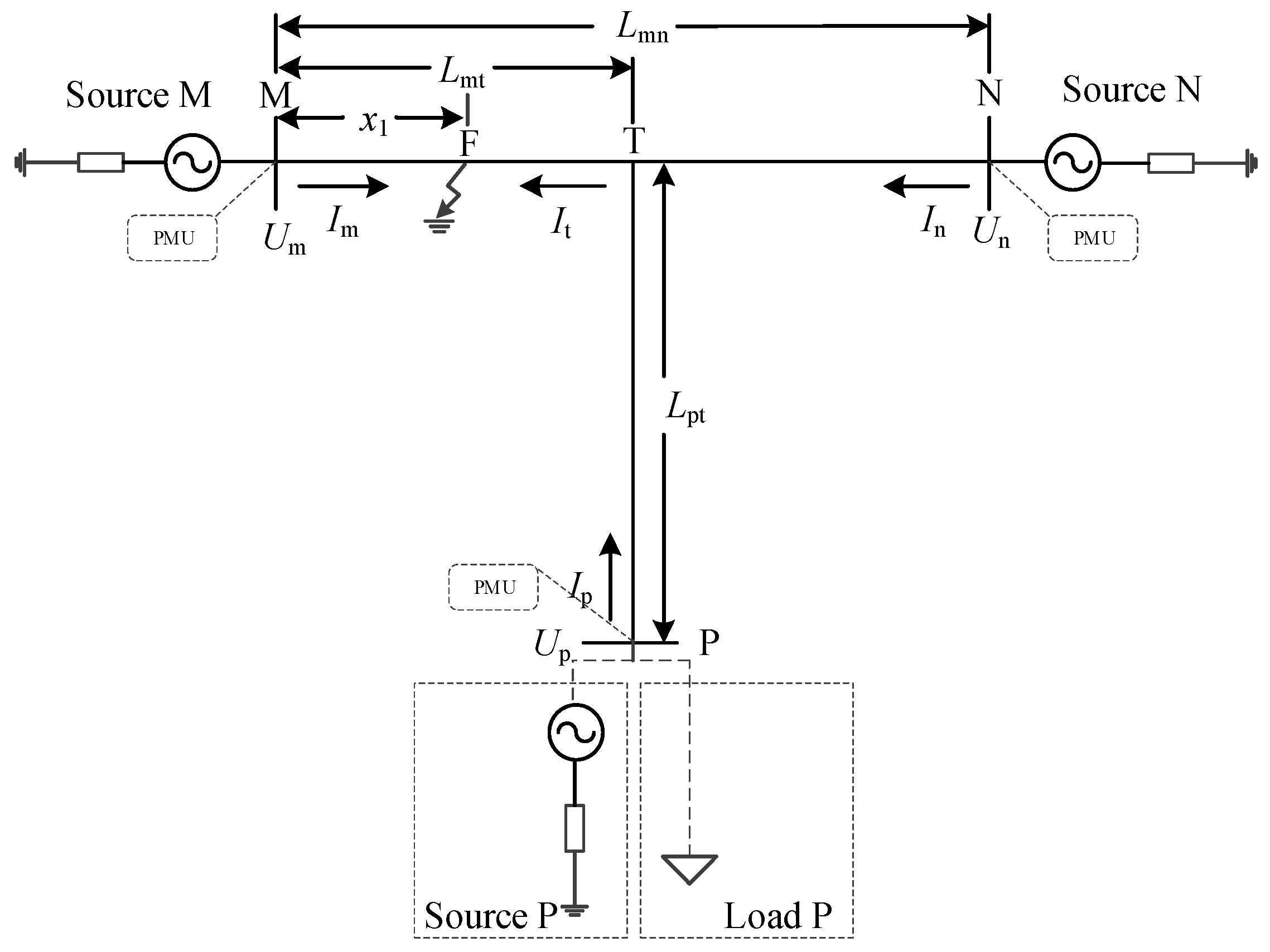
Considering that T-type transmission lines of a distribution network are usually short, this algorithm assumes that transmission lines are fully transposed and neglects the shunt capacitances [6]. However, the Π-type equivalent line model is still adopted for simulation verification. T-type transmission line is usually divided into two types, namely three-terminal line and tapped line, where the former means the branch line is fed by a power source and the latter means the branch line is terminated at loads [16]. These two structures are all shown in Figure 1. In this paper, the line from terminal M to N and the line from tapping point T to terminal P are denoted as the main line and branch line, respectively, where each have different parameters. Each terminal is equipped with a μMPMU and the measurements are synchronous.

Assuming the fault occurs on the section MT, the current flowing from the terminal M to point F is $I_{\mathrm{m}}$. The current $I_{\mathrm{t}}$ flowing from point T to point F is the sum of the current $I_{\mathrm{n}}$ flowing from terminal N to point T and the current $I_{\mathrm{p}}$ flowing from terminal P to point T, as shown in Equation (1):

$$I_{\mathrm{t}}=I_{\mathrm{p}}+I_{\mathrm{n}}$$

(1)

The post-fault three-phase voltages of point F derived using the voltage and current measured at terminals M, N, and P are equal. Then, the equations derived based on the above principle, as shown in Equations (2)–(7), are:

$$\begin{array}{ll}{U}_{\mathrm{ma}}-I_{\mathrm{ma}}{z}_{\mathrm{s}1}{x}_1& -I_{\mathrm{mb}}{z}_{\mathrm{m}1}{x}_1-I_{\mathrm{mc}}{z}_{\mathrm{m}1}{x}_1\\ & =U_{\mathrm{na}}-I_{\mathrm{na}}{z}_{\mathrm{s}1}\left(L_{\mathrm{mn}}-L_{\mathrm{mt}}\right)-I_{\mathrm{nb}}{z}_{\mathrm{m}1}\left(L_{\mathrm{mn}}-L_{\mathrm{mt}}\right)\\ & -I_{\mathrm{nc}}{z}_{\mathrm{m}1}\left(L_{\mathrm{mn}}-L_{\mathrm{mt}}\right)-(I_{\mathrm{na}}+I_{\mathrm{pa}})z_{\mathrm{s}1}\left(L_{\mathrm{mt}}-x_1\right)\\ & -(I_{\mathrm{nb}}+I_{\mathrm{pb}})z_{\mathrm{m}1}\left(L_{\mathrm{mt}}-x_1\right)-\left(I_{\mathrm{nc}}+I_{\mathrm{pc}}\right)z_{\mathrm{m}1}\left(L_{\mathrm{mt}}-x_1\right)\end{array}$$

(2)

$$\begin{array}{ll}{U}_{\mathrm{mb}}-I_{\mathrm{mb}}{z}_{\mathrm{s}1}{x}_1& -I_{\mathrm{ma}}{z}_{\mathrm{m}1}{x}_1-I_{\mathrm{mc}}{z}_{\mathrm{m}1}{x}_1\\ & =U_{\mathrm{nb}}-I_{\mathrm{nb}}{z}_{\mathrm{s}1}\left(L_{\mathrm{mn}}-L_{\mathrm{mt}}\right)-I_{\mathrm{na}}{z}_{\mathrm{m}1}\left(L_{\mathrm{mn}}-L_{\mathrm{mt}}\right)\\ & -I_{\mathrm{nc}}{z}_{\mathrm{m}1}\left(L_{\mathrm{mn}}-L_{\mathrm{mt}}\right)-(I_{\mathrm{nb}}+I_{\mathrm{pb}})z_{\mathrm{s}1}\left(L_{\mathrm{mt}}-x_1\right)\\ & -(I_{\mathrm{na}}+I_{\mathrm{pa}})z_{\mathrm{m}1}\left(L_{\mathrm{mt}}-x_1\right)-\left(I_{\mathrm{nc}}+I_{\mathrm{pc}}\right)z_{\mathrm{m}1}\left(L_{\mathrm{mt}}-x_1\right)\end{array}$$

(3)

$$\begin{array}{ll}{U}_{\mathrm{mc}}-I_{\mathrm{mc}}{z}_{\mathrm{s}1}{x}_1& -I_{\mathrm{ma}}{z}_{\mathrm{m}1}{x}_1-I_{\mathrm{mb}}{z}_{\mathrm{m}1}{x}_1=U_{\mathrm{nc}}-I_{\mathrm{nc}}{z}_{\mathrm{s}1}\left(L_{\mathrm{mn}}-L_{\mathrm{mt}}\right)\\ & -I_{\mathrm{na}}{z}_{\mathrm{m}1}\left(L_{\mathrm{mn}}-L_{\mathrm{mt}}\right)-I_{\mathrm{nb}}{z}_{\mathrm{m}1}\left(L_{\mathrm{mn}}-L_{\mathrm{mt}}\right)-\left(I_{\mathrm{nc}}+I_{\mathrm{pc}}\right)z_{\mathrm{s}1}(L_{\mathrm{mt}}-x_1)\\ & -(I_{\mathrm{na}}+I_{\mathrm{pa}})z_{\mathrm{m}1}\left(L_{\mathrm{mt}}-x_1\right)-\left(I_{\mathrm{nb}}+I_{\mathrm{pb}}\right)z_{\mathrm{m}1}\left(L_{\mathrm{mt}}-x_1\right)\end{array}$$

(4)

$$\begin{array}{ll}{U}_{\mathrm{ma}}-I_{\mathrm{ma}}{z}_{\mathrm{s}1}{x}_1& -I_{\mathrm{mb}}{z}_{\mathrm{m}1}{x}_1-I_{\mathrm{mc}}{z}_{\mathrm{m}1}{x}_1=U_{\mathrm{pa}}-I_{\mathrm{pa}}{z}_{\mathrm{s}2}{L}_{\mathrm{pt}}-I_{\mathrm{pb}}{z}_{\mathrm{m}2}{L}_{\mathrm{pt}}-I_{\mathrm{pc}}{z}_{\mathrm{m}2}{L}_{\mathrm{pt}}\\ & -\left(I_{\mathrm{na}}+I_{\mathrm{pa}}\right)z_{\mathrm{s}1}\left(L_{\mathrm{mt}}-x_1\right)-\left(I_{\mathrm{nb}}+I_{\mathrm{pb}}\right)z_{\mathrm{m}1}\left(L_{\mathrm{mt}}-x_1\right)\\ & -(I_{\mathrm{nc}}+I_{\mathrm{pc}})z_{\mathrm{m}1}\left(L_{\mathrm{mt}}-x_1\right)\end{array}$$

(5)

$$\begin{array}{ll}{U}_{\mathrm{mb}}-I_{\mathrm{mb}}{z}_{\mathrm{s}1}{x}_1& -I_{\mathrm{ma}}{z}_{\mathrm{m}1}{x}_1-I_{\mathrm{mc}}{z}_{\mathrm{m}1}{x}_1\\ & =U_{\mathrm{pb}}-I_{\mathrm{pb}}{z}_{\mathrm{s}2}{L}_{\mathrm{pt}}-I_{\mathrm{pa}}{z}_{\mathrm{m}2}{L}_{\mathrm{pt}}-I_{\mathrm{pc}}{z}_{\mathrm{m}2}{L}_{\mathrm{pt}}-\left(I_{\mathrm{nb}}+I_{\mathrm{pb}}\right)z_{\mathrm{s}1}(L_{\mathrm{mt}}-x_1)\\ & -(I_{\mathrm{na}}+I_{\mathrm{pa}})z_{\mathrm{m}1}\left(L_{\mathrm{mt}}-x_1\right)-\left(I_{\mathrm{nc}}+I_{\mathrm{pc}}\right)z_{\mathrm{m}1}\left(L_{\mathrm{mt}}-x_1\right)\end{array}$$

(6)

$$\begin{array}{ll}{U}_{\mathrm{mc}}-I_{\mathrm{mc}}{z}_{\mathrm{s}1}{x}_1& -I_{\mathrm{ma}}{z}_{\mathrm{m}1}{x}_1-I_{\mathrm{mb}}{z}_{\mathrm{m}1}{x}_1\\ & =U_{\mathrm{pc}}-I_{\mathrm{pc}}{z}_{\mathrm{s}2}{L}_{\mathrm{pt}}-I_{\mathrm{pa}}{z}_{\mathrm{m}2}{L}_{\mathrm{pt}}-I_{\mathrm{pb}}{z}_{\mathrm{m}2}{L}_{\mathrm{pt}}-\left(I_{\mathrm{nc}}+I_{\mathrm{pc}}\right)z_{\mathrm{s}1}\left(L_{\mathrm{mt}}-x_1\right)\\ & -(I_{\mathrm{na}}+I_{\mathrm{pa}})z_{\mathrm{m}1}\left(L_{\mathrm{mt}}-x_1\right) - \left(I_{\mathrm{nb}}+I_{\mathrm{pb}}\right)z_{\mathrm{m}1}\left(L_{\mathrm{mt}}-x_1\right)\end{array}$$

(7)

where:

$U_{\mathrm{ma},\mathrm{b},\mathrm{c}}$	post-fault phase voltage at the terminal M
$U_{\mathrm{na},\mathrm{b},\mathrm{c}}$	post-fault phase voltage at the terminal N
$U_{\mathrm{pa},\mathrm{b},\mathrm{c}}$	post-fault phase voltage at the terminal P
$I_{\mathrm{ma},\mathrm{b},\mathrm{c}}$	post-fault phase current flowing from the terminal M
$I_{\mathrm{na},\mathrm{b},\mathrm{c}}$	post-fault phase current flowing from the terminal N
$I_{\mathrm{pa},\mathrm{b},\mathrm{c}}$	post-fault phase current flowing from the terminal P
$x_1$	fault distance between fault point F and terminal M
$L_{\mathrm{mn}}$	distance between terminal M and terminal N
$L_{\mathrm{mt}}$	distance between terminal M and point T
$L_{\mathrm{pt}}$	distance between terminal P and point T
$z_{\mathrm{s}1}$	self-impedance per unit length of line MN
$z_{\mathrm{m}1}$	mutual impedance per unit length of line MN
$z_{\mathrm{s}2}$	self-impedance per unit length of line PT
$z_{\mathrm{m}2}$	mutual impedance per unit length of line PT

To simplify the formulae, the following definitions are given:

$${\mathit{U}}_m=\left[\begin{array}{c}{U}_{\mathrm{ma}}\\ U_{\mathrm{mb}}\\ U_{\mathrm{mc}}\end{array}\right] {\mathit{U}}_n=\left[\begin{array}{c}{U}_{\mathrm{na}}\\ U_{\mathrm{nb}}\\ U_{\mathrm{nc}}\end{array}\right] {\mathit{U}}_p=\left[\begin{array}{c}{U}_{\mathrm{pa}}\\ U_{\mathrm{pb}}\\ U_{\mathrm{pc}}\end{array}\right]$$

(8)

$${\mathit{I}}_m=\left[\begin{array}{c}{I}_{\mathrm{ma}}\\ I_{\mathrm{mb}}\\ I_{\mathrm{mc}}\end{array}\right] {\mathit{I}}_n=\left[\begin{array}{c}{I}_{\mathrm{na}}\\ I_{\mathrm{nb}}\\ I_{\mathrm{nc}}\end{array}\right] {\mathit{I}}_p=\left[\begin{array}{c}{I}_{\mathrm{pa}}\\ I_{\mathrm{pb}}\\ I_{\mathrm{pc}}\end{array}\right]$$

(9)

$${\mathit{z}}_{\mathbf{1}}=\left[\begin{array}{ccc}{z}_{\mathrm{s}1}& z_{\mathrm{m}1}& z_{\mathrm{m}1}\\ z_{\mathrm{m}1}& z_{\mathrm{s}1}& z_{\mathrm{m}1}\\ z_{\mathrm{m}1}& z_{\mathrm{m}1}& z_{\mathrm{s}1}\end{array}\right] {\mathit{z}}_{\mathbf{2}}=\left[\begin{array}{ccc}{z}_{\mathrm{s}2}& z_{\mathrm{m}2}& z_{\mathrm{m}2}\\ z_{\mathrm{m}2}& z_{\mathrm{s}2}& z_{\mathrm{m}2}\\ z_{\mathrm{m}2}& z_{\mathrm{m}2}& z_{\mathrm{s}2}\end{array}\right]$$

(10)

Then Equations (2)–(7) are simplified to Equation (11):

$$\begin{array}{c}{\mathit{U}}_m-{\mathit{z}}_{\mathbf{1}}{\mathit{I}}_m{x}_1={\mathit{U}}_n-{\mathit{z}}_{\mathbf{1}}{\mathit{I}}_n\left(L_{\mathrm{mn}}-L_{\mathrm{mt}}\right)-{\mathit{z}}_{\mathbf{1}}\left({\mathit{I}}_n+{\mathit{I}}_p\right)\left(L_{\mathrm{mt}}-x_1\right)\\ {\mathit{U}}_m-{\mathit{z}}_{\mathbf{1}}{\mathit{I}}_m{x}_1={\mathit{U}}_p-{\mathit{z}}_{\mathbf{2}}{\mathit{I}}_p{L}_{\mathrm{pt}}-{\mathit{z}}_{\mathbf{1}}\left({\mathit{I}}_n+{\mathit{I}}_p\right)\left(L_{\mathrm{mt}}-x_1\right)\end{array}$$

(11)

Assuming the fault occurs on the section NT, the following equations can also be derived, as given in Equation (12).

$$\begin{array}{c}{\mathit{U}}_n-{\mathit{z}}_{\mathbf{1}}{\mathit{I}}_n{x}_2={\mathit{U}}_m-{\mathit{z}}_{\mathbf{1}}{\mathit{I}}_m{L}_{\mathrm{mt}}-{\mathit{z}}_{\mathbf{1}}\left({\mathit{I}}_m+{\mathit{I}}_p\right)\left(L_{\mathrm{mn}}-L_{\mathrm{mt}}-x_2\right)\\ {\mathit{U}}_n-{\mathit{z}}_{\mathbf{1}}{\mathit{I}}_n{x}_2={\mathit{U}}_p-{\mathit{z}}_{\mathbf{2}}{\mathit{I}}_p{L}_{\mathrm{pt}}-{\mathit{z}}_{\mathbf{1}}\left({\mathit{I}}_m+{\mathit{I}}_p\right)\left(L_{\mathrm{mn}}-L_{\mathrm{mt}}-x_2\right)\end{array}$$

(12)

where $x_2$ is the fault distance between fault point F and terminal N.

Assuming the fault occurs on the section PT, Equation (13) can be given similarly.

$$\begin{array}{c}{\mathit{U}}_p-{\mathit{z}}_{\mathbf{2}}{\mathit{I}}_p{x}_3={\mathit{U}}_m-{\mathit{z}}_{\mathbf{1}}{\mathit{I}}_m{L}_{\mathrm{mt}}-{\mathit{z}}_{\mathbf{2}}\left({\mathit{I}}_m+{\mathit{I}}_n\right)\left(L_{\mathrm{pt}}-x_3\right)\\ {\mathit{U}}_p-{\mathit{z}}_{\mathbf{2}}{\mathit{I}}_p{x}_3={\mathit{U}}_n-{\mathit{z}}_{\mathbf{1}}{\mathit{I}}_n(L_{\mathrm{mn}}-L_{\mathrm{mt}})-{\mathit{z}}_{\mathbf{2}}\left({\mathit{I}}_m+{\mathit{I}}_n\right)\left(L_{\mathrm{pt}}-x_3\right)\end{array}$$

(13)

where $x_3$ is the fault distance between fault point F and terminal P.

For each assumed faulty section, an equation set consisting of six non-linear equations (e.g., Equations (2)–(7)) with six unknowns (fault distance, distance between M and T, self-impedance, and mutual impedance per unit length of line MN and PT) can be established on the basis of three-terminal synchronous fundamental frequency components. There are as many equations as unknowns, so each equation set can be solved using a suitable numerical algorithm.

2.2. Improvement of Fault Location Equations

The aforementioned fault location algorithm can accurately locate the fault without line parameter values under the premise of precisely obtaining the fundamental frequency voltages, currents, and each line length. However, in engineering practice, the data error caused by the measurement, background noise, and phasor calculation will inevitably exist. Hence, the data entered into the algorithm are inaccurate, which would greatly affect the accuracy of the algorithm and could cause the algorithm to fail. Therefore, the algorithm needs to be improved to reduce the influence of data error.

When data error exists, a single equation set (e.g., Equation (11)) could yield the fault location result with considerable error. However, redundant equation sets can be built by using different sets of fundamental frequency data, which are obtained by different sets of sampling data. Then, the solving of equation sets is transformed into a global optimization problem, and the influence of data error can be reduced to some extent based on estimation theory.

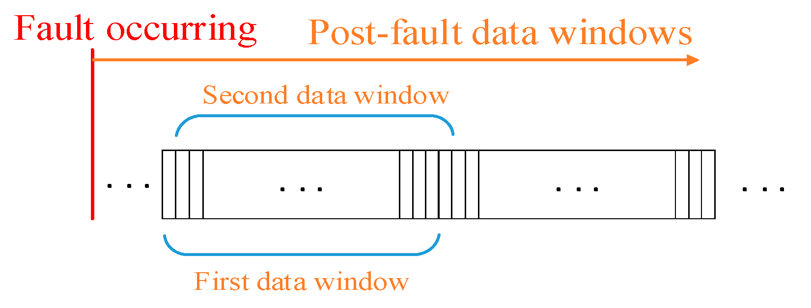
Different sets of sampling data can be constructed by sliding the data window, which is illustrated in Figure 2.

Considering the effects of the decaying direct current component and the action time of the relay protection equipment, only the post-fault second and third cycle of sampling data in the measurement devices are used. One cycle of voltage and current data consists of 128 sampling values in this paper. First, starting from the first sampling value of the second cycle of sampling data after the fault, a total of 128 sampling values are selected to form the first data window, and the corresponding fundamental voltage and current are extracted using a DFT algorithm to construct one set of equations. Then, the data window is slid over one sampling period step to extract the corresponding fundamental voltage and current. The fundamental voltage and current of the M, N, and P terminals extracted using the s-th data window are defined as follows: $U_{\mathrm{m}s}, U_{\mathrm{n}s}$,$U_{\mathrm{p}s}, I_{\mathrm{m}s}, I_{\mathrm{n}s}, I_{\mathrm{p}s},s=1, 2,\dots ,j$.

Thus, assuming a fault occurs on the MT section, j equation sets can be constructed as shown in Equation (14):

$$\begin{gathered} {\mathit{U}}_{m\mathbf{1}}-{\mathit{z}}_{\mathbf{1}}{\mathit{I}}_{m\mathbf{1}}{x}_1={\mathit{U}}_{n\mathbf{1}}-{\mathit{z}}_{\mathbf{1}}{\mathit{I}}_{n\mathbf{1}}\left(L_{\mathrm{mn}}-L_{\mathrm{mt}}\right)-{\mathit{z}}_{\mathbf{1}}\left({\mathit{I}}_{n\mathbf{1}}+{\mathit{I}}_{p\mathbf{1}}\right)\left(L_{\mathrm{mt}}-x_1\right) \\ {\mathit{U}}_{m\mathbf{1}}-{\mathit{z}}_{\mathbf{1}}{\mathit{I}}_{m\mathbf{1}}{x}_1={\mathit{U}}_{p\mathbf{1}}-{\mathit{z}}_{\mathbf{2}}{\mathit{I}}_{p\mathbf{1}}{L}_{\mathrm{pt}}-{\mathit{z}}_{\mathbf{1}}\left({\mathit{I}}_{n\mathbf{1}}+{\mathit{I}}_{p\mathbf{1}}\right)\left(L_{\mathrm{mt}}-x_1\right) \\ ⋮ \\ {\mathit{U}}_{m\mathit{j}}-{\mathit{z}}_{\mathbf{1}}{\mathit{I}}_{m\mathit{j}}{x}_1={\mathit{U}}_{n\mathit{j}}-{\mathit{z}}_{\mathbf{1}}{\mathit{I}}_{n\mathit{j}}\left(L_{\mathrm{mn}}-L_{\mathrm{mt}}\right)-{\mathit{z}}_{\mathbf{1}}\left({\mathit{I}}_{n\mathit{j}}+{\mathit{I}}_{p\mathit{j}}\right)\left(L_{\mathrm{mt}}-x_1\right) \\ {\mathit{U}}_{m\mathit{j}}-{\mathit{z}}_{\mathbf{1}}{\mathit{I}}_{m\mathit{j}}{x}_1={\mathit{U}}_{p\mathit{j}}-{\mathit{z}}_{\mathbf{2}}{\mathit{I}}_{p\mathit{j}}{L}_{\mathrm{pt}}-{\mathit{z}}_{\mathbf{1}}\left({\mathit{I}}_{n\mathit{j}}+{\mathit{I}}_{p\mathit{j}}\right)\left(L_{\mathrm{mt}}-x_1\right) \end{gathered}$$

(14)

Similarly, assuming a fault occurs on the NT section, equations shown in Equation (15) can be built:

$$\begin{gathered} {\mathit{U}}_{n\mathbf{1}}-{\mathit{z}}_{\mathbf{1}}{\mathit{I}}_{n\mathbf{1}}{x}_2={\mathit{U}}_{m\mathbf{1}}-{\mathit{z}}_{\mathbf{1}}{\mathit{I}}_{m\mathbf{1}}{L}_{\mathrm{mt}}-{\mathit{z}}_{\mathbf{1}}\left({\mathit{I}}_{m\mathbf{1}}+{\mathit{I}}_{p\mathbf{1}}\right)\left(L_{\mathrm{mn}}-L_{\mathrm{mt}}-x_2\right) \\ {\mathit{U}}_{n\mathbf{1}}-{\mathit{z}}_{\mathbf{1}}{\mathit{I}}_{n\mathbf{1}}{x}_2={\mathit{U}}_{p\mathbf{1}}-{\mathit{z}}_{\mathbf{2}}{\mathit{I}}_{p\mathbf{1}}{L}_{\mathrm{pt}}-{\mathit{z}}_{\mathbf{1}}\left({\mathit{I}}_{m\mathbf{1}}+{\mathit{I}}_{p\mathbf{1}}\right)\left(L_{\mathrm{mn}}-L_{\mathrm{mt}}-x_2\right) \\ ⋮ \\ {\mathit{U}}_{n\mathit{j}}-{\mathit{z}}_{\mathbf{1}}{\mathit{I}}_{n\mathit{j}}{x}_2={\mathit{U}}_{m\mathit{j}}-{\mathit{z}}_{\mathbf{1}}{\mathit{I}}_{m\mathit{j}}{L}_{\mathrm{mt}}-{\mathit{z}}_{\mathbf{1}}\left({\mathit{I}}_{m\mathit{j}}+{\mathit{I}}_{p\mathit{j}}\right)\left(L_{\mathrm{mn}}-L_{\mathrm{mt}}-x_2\right) \\ {\mathit{U}}_{n\mathit{j}}-{\mathit{z}}_{\mathbf{1}}{\mathit{I}}_{n\mathit{j}}{x}_2={\mathit{U}}_{p\mathit{j}}-{\mathit{z}}_{\mathbf{2}}{\mathit{I}}_{p\mathit{j}}{L}_{\mathrm{pt}}-{\mathit{z}}_{\mathbf{1}}\left({\mathit{I}}_{m\mathit{j}}+{\mathit{I}}_{p\mathit{j}}\right)\left(L_{\mathrm{mn}}-L_{\mathrm{mt}}-x_2\right) \end{gathered}$$

(15)

Assuming a fault occurs on the PT section, the following Equation (16) can be established:

$$\begin{gathered} {\mathit{U}}_{p\mathbf{1}}-{\mathit{z}}_{\mathbf{2}}{\mathit{I}}_{p\mathbf{1}}{x}_3={\mathit{U}}_{m\mathbf{1}}-{\mathit{z}}_{\mathbf{1}}{\mathit{I}}_{m\mathbf{1}}{L}_{\mathrm{mt}}-{\mathit{z}}_{\mathbf{2}}\left({\mathit{I}}_{m\mathbf{1}}+{\mathit{I}}_{n\mathbf{1}}\right)\left(L_{\mathrm{pt}}-x_3\right) \\ {\mathit{U}}_{p\mathbf{1}}-{\mathit{z}}_{\mathbf{2}}{\mathit{I}}_{p\mathbf{1}}{x}_3={\mathit{U}}_{n\mathbf{1}}-{\mathit{z}}_{\mathbf{1}}{\mathit{I}}_{n\mathbf{1}}(L_{\mathrm{mn}}-L_{\mathrm{mt}})-{\mathit{z}}_{\mathbf{2}}\left({\mathit{I}}_{m\mathbf{1}}+{\mathit{I}}_{n\mathbf{1}}\right)\left(L_{\mathrm{pt}}-x_3\right) \\ ⋮ \\ {\mathit{U}}_{p\mathit{j}}-{\mathit{z}}_{\mathbf{2}}{\mathit{I}}_{p\mathit{j}}{x}_3={\mathit{U}}_{m\mathit{j}}-{\mathit{z}}_{\mathbf{1}}{\mathit{I}}_{m\mathit{j}}{L}_{\mathrm{mt}}-{\mathit{z}}_{\mathbf{2}}\left({\mathit{I}}_{m\mathit{j}}+{\mathit{I}}_{n\mathit{j}}\right)\left(L_{\mathrm{pt}}-x_3\right) \\ {\mathit{U}}_{p\mathit{j}}-{\mathit{z}}_{\mathbf{2}}{\mathit{I}}_{p\mathit{j}}{x}_3={\mathit{U}}_{n\mathit{j}}-{\mathit{z}}_{\mathbf{1}}{\mathit{I}}_{n\mathit{j}}(L_{\mathrm{mn}}-L_{\mathrm{mt}})-{\mathit{z}}_{\mathbf{2}}\left({\mathit{I}}_{m\mathit{j}}+{\mathit{I}}_{n\mathbf{j}}\right)\left(L_{\mathrm{pt}}-x_3\right) \end{gathered}$$

(16)

where $x_1$, $x_2$, $x_3$, ${\mathit{z}}_{\mathbf{1}}$, ${\mathit{z}}_{\mathbf{2}}$, $L_{\mathrm{mt}}$, $L_{\mathrm{mn}}$, $L_{\mathrm{pt}}$ have the same meaning as that in Equations (11)–(13).

The equations corresponding to each assumed faulty section involve six unknowns, that is, $x_1$ ($\mathrm{or} x_2 \mathrm{or} x_3$), $L_{\mathrm{mt}}$,$z_{\mathrm{s}1}$, $z_{\mathrm{m}1}$, $z_{\mathrm{s}2}$, and $z_{\mathrm{m}2}$. As such, the overdetermined Equations (14)–(16) can be solved using a numerical algorithm. The details of solving via a trust-region algorithm are illustrated in Section 2.3. Considering the speed of solving and accuracy of the solution, j is set to 30 in the proposed fault location algorithm.

2.3. Solving the Fault Location Equations

The basic idea of the Newton-Raphson method is to approximate the objective function with its second-order Taylor series around the iteration point $t_k$, and use the minimum value $s_k$ to correct $t_k$. This method can only guarantee local convergence and may fail to give the solution if the initial value is improper.

By contrast, the basic idea of the trust-region algorithm is to set $t_k$ as the current iteration value and solve a sub-problem in a closed spherical trust region with $t_k$ as the center and $r_k$ as the radius to obtain the trial step size $d_k$. If the trial is successful, in the next iteration, the radius of the trust region remains unchanged or expands, and $t_k$ is updated to $t_k+d_k$. Otherwise, the radius is reduced and $t_k$ does not change. Therefore, the trust region algorithm needs to continuously update the trial step size $d_k$, the trust region radius $r_k$, and the iteration value $t_k$ until the objective function converges.

The trust-region algorithm can directly determine the search area and dynamically correct it, producing a global convergence with higher robustness, which can guarantee a solution whenever it exists [21]. Therefore, in order to realize the solving of fault location equations more reliably, a trust-region algorithm is preferred in this paper. Equation (14) corresponding to the fault on section MT is taken as an example to describe the solving process. Here, j is set to 1 for the convenience of explanation.

If j is equal to 1, the Equation (14) contains six equations (i.e., Equations (2)–(7)) involving complex variables. When the trust-region algorithm is used, the six equations in the complex domain need to be transformed into 12 equations in the real domain by separating the real and imaginary parts. If $z_{\mathrm{s}1}$, $z_{\mathrm{m}1}$, $z_{\mathrm{s}2}$, and $z_{\mathrm{m}2}$ are respectively represented as $r_{\mathrm{s}1}+\mathrm{j}\times l_{\mathrm{s}1}$, $r_{\mathrm{m}1}+\mathrm{j}\times l_{\mathrm{m}1}$, $r_{\mathrm{s}2}+\mathrm{j}\times l_{\mathrm{s}2}$, and $r_{\mathrm{m}2}+\mathrm{j}\times l_{\mathrm{m}2}$, the unknowns $x_1$, $L_{\mathrm{mt}}$, $z_{\mathrm{s}1}$, $z_{\mathrm{m}1}$, and $z_{\mathrm{s}2}$, $z_{\mathrm{m}2}$ will be transformed into $x_1$, $L_{\mathrm{mt}}$, $r_{\mathrm{s}1}$, $l_{\mathrm{s}1}$, $r_{\mathrm{m}1}$, $l_{\mathrm{m}1}$, $r_{\mathrm{s}2}$, $l_{\mathrm{s}2}$, $r_{\mathrm{m}2}$, and $l_{\mathrm{m}2}$ accordingly.

First, define the unknown variable vector:

$$t=[x_1,L_{\mathrm{mt}},r_{\mathrm{s}1},l_{s1},r_{\mathrm{m}1},l_{\mathrm{m}1},r_{\mathrm{s}2},l_{s2},r_{\mathrm{m}2},l_{\mathrm{m}2}]$$

(17)

Then, Equation (14) can be expressed as Equation (18):

$$\{\begin{array}{c}{f}_1(t)=0\\ f_2(t)=0\\ ⋮\\ f_{12}(t)=0\end{array}$$

(18)

Now, make another definition as follows:

$$g(t)=[f_1(t),f_2(t),\cdots ,f_{12}(t)]$$

(19)

Therefore, the solving of the equations can be transformed into a minimization problem in the form of Equation (20), where $\Vert g\left(t\right)\Vert =\sqrt{g\left(t\right)\times g{\left(t\right)}^T}$:

$$\min h(t)=\frac{1}{2}{\Vert g(t)\Vert }^2$$

(20)

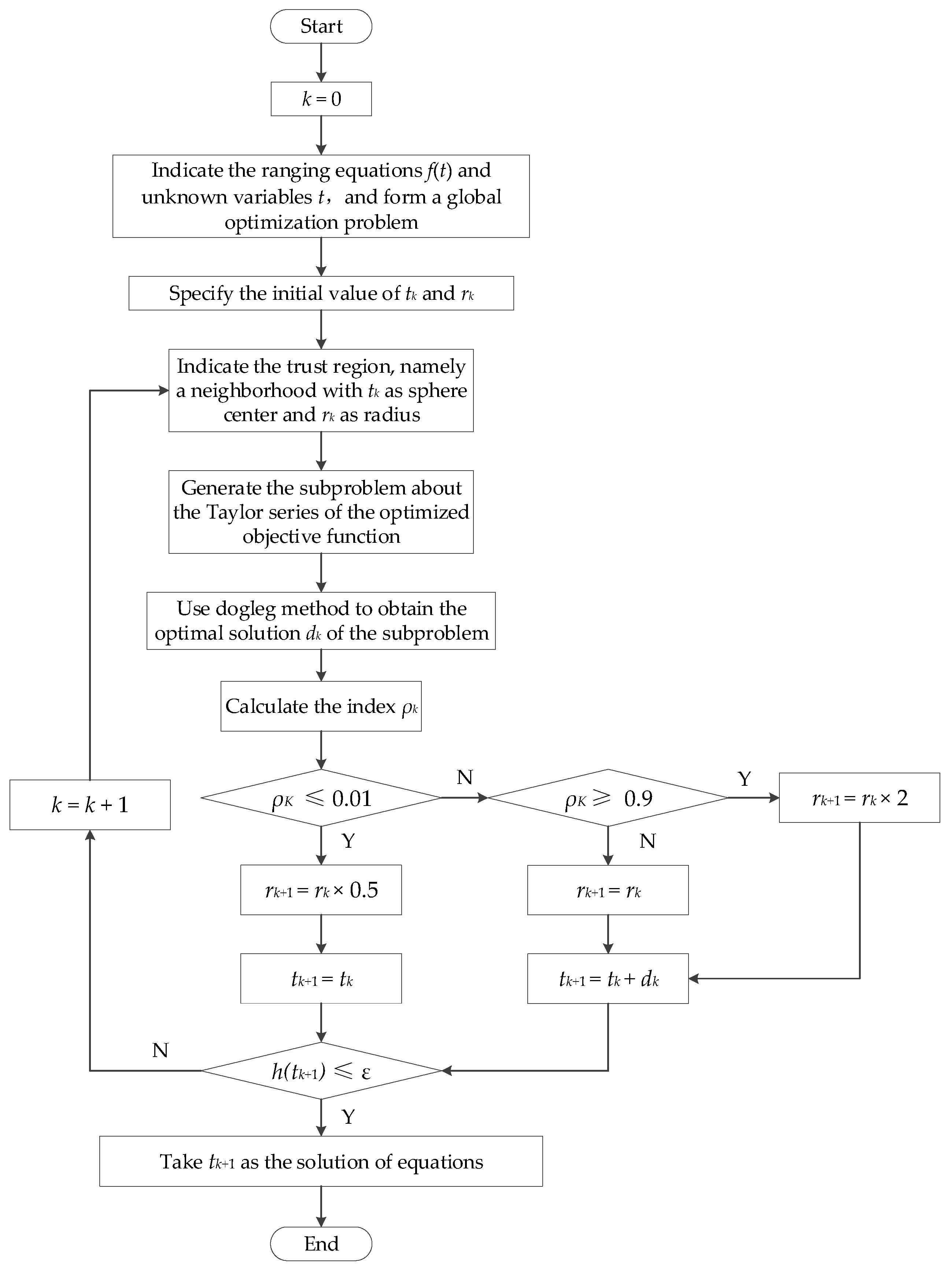
When the trust-region algorithm is used to solve the minimization problem, a trial step size $d_k$, a trust region radius $r_k$ and an iteration value $t_k$ need to be specified for each iteration. The initial value $t_0$ and $r_0$ can be set to 1 here due to the low initial value requirement of the algorithm.

2.3.1. Calculation of $d_k$

The step size $d_k$ is calculated by solving the following optimization sub-problem, as given in Equation (21), by attempting to make $h(t_k+d_k)$ smaller than $h\left(t_k\right)$, where, $q_k\left(d_k\right)$ is the second-order Taylor series of $h\left(t\right)$ around $t_k$ and its behavior approximates to $h(t_k)$. $\nabla h(t_k)$ and ${\nabla }^{2}h(t_k)$ respectively represent the gradient and Hessian of $h\left(t\right)$ at $t_k$. The superscript T represents matrix transposition.

$$\begin{array}{c}\min q_k(d_k)=h(t_k)+\nabla h{(t_k)}^{\mathrm{T}}{d}_k+\frac{1}{2}{d}_k{}^{\mathrm{T}}{\nabla }^{2}h(t_k)d_k\\ s.t. \Vert d_k\Vert \le r_k\end{array}$$

(21)

Due to its great effect, the dogleg algorithm is used in this paper to solve the sub-problem [21]. The details are as follows:

First, define two variables $B_k$ and $U_k$, so as to obtain the index ${\tau }_k$:

$$B_k=-{({\nabla }^{2}h(t_k))}^{-1}\cdot \nabla h(t_k)$$

(22)

$$U_k=-\frac{{({\nabla }^{2}h(t_k))}^{\mathrm{T}}\cdot \nabla h(t_k)}{{({\nabla }^{2}h(t_k))}^T\cdot {\nabla }^{2}h(t_k)\cdot \nabla h(t_k)}\nabla h(t_k)$$

(23)

If $\Vert U_k\Vert \ge r_k$, ${\tau }_k$ is updated to ${\tau }_k/\Vert U_k\Vert$. If $\Vert B_k\Vert \ge r_k$, ${\tau }_k$ is updated to $\sqrt{\left(r_k^2-U_k^{\mathrm{T}}{U}_k\right)/({\left(B_k-U_k\right)}^{\mathrm{T}}\times \left(B_k-U_k\right))}+1$. Otherwise, ${\tau }_k$ is set to 2.

Finally, if ${\tau }_k$ is smaller than 1, $d_k={\tau }_k\times U_k$. Otherwise, $d_k=U_k+\left({\tau }_k-1\right)\times \left(B_k-U_k\right)$.

2.3.2. Calculation of $r_k$ and $t_k$

The adjustment of the trust region radius $r_k$ and the update of the iteration value $t_k$ are based on the built index ${\rho }_k$.

$${\rho }_k=\frac{h\left(t_k\right)-h\left(t_k+d_k\right)}{q_k\left(0\right)-q_k\left(d_k\right)}$$

(24)

If ${\rho }_k\ge 0.9$, this means that $q_k\left(d_k\right)$ can effectively reflect the behavior of $h(t_k)$. In order to improve the convergence speed, the radius $r_k$ is set to $2\times r_k$. If ${\rho }_k\le 0.01$, this means that the approximation of $q_k\left(d_k\right)$ is not effective, so $r_k$ is set to $0.5\times r_k$. Otherwise, $r_k$ remains unchanged.

Furthermore, if ${\rho }_k>0.01$, this indicates that the objective function value is successfully reduced. Then, the solution is modified with the trial step size, that is, $t_{k+1}=t_k+d_k$. Otherwise, $t_k$ is not modified.

2.3.3. Determination of the Solution

The iteration process continues until the convergence condition is satisfied, that is, $h(t_{k+1})\le \mathsf{\epsilon }$. Finally, $t_{k+1}$ is taken as the solution of Equation (14). The flowchart of solving using the trust-region algorithm is shown in Figure 3.

2.4. Identification of the Fault Point

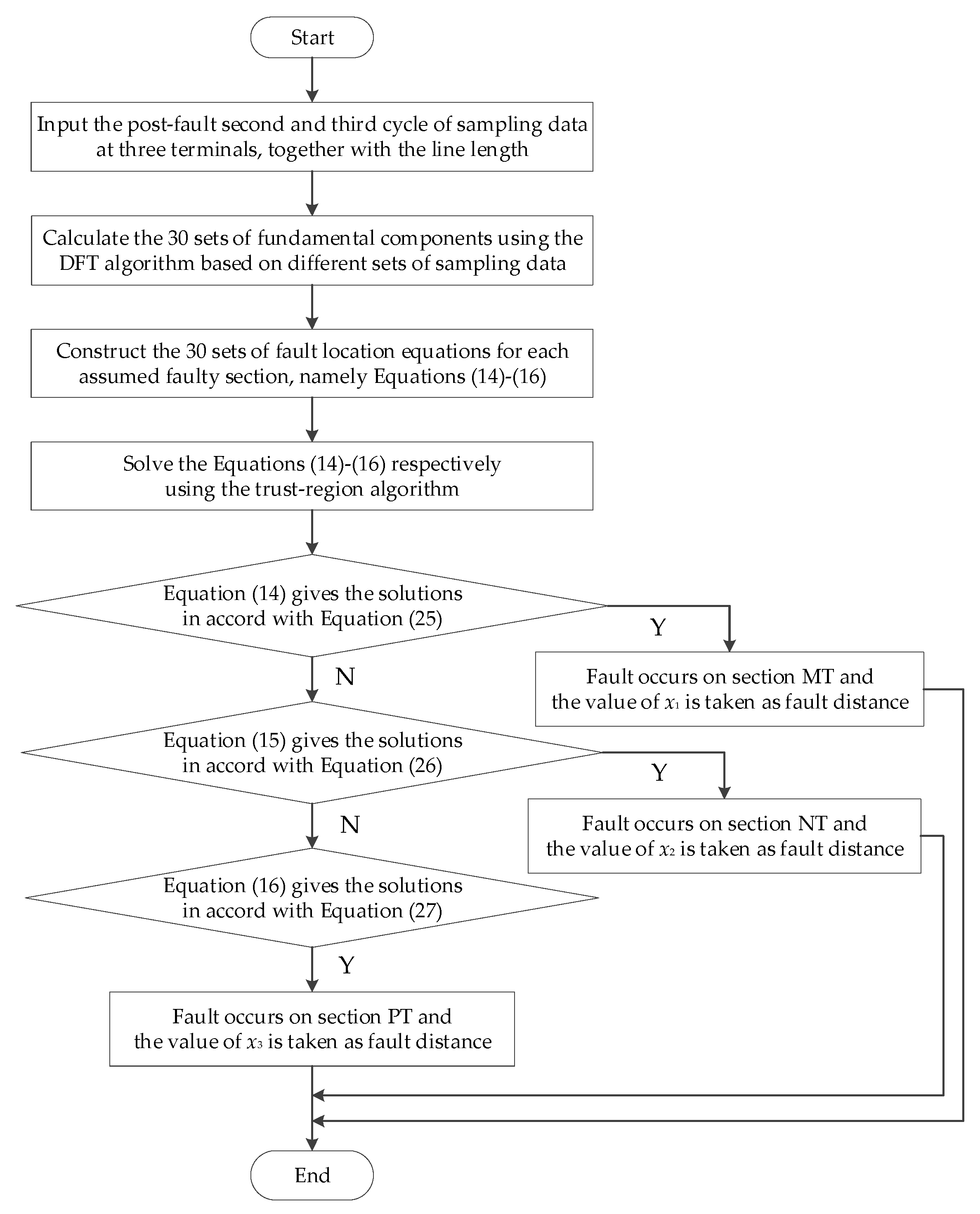
Regardless of which section the fault occurs on, Equations (14)–(16) can all be tried to solve the trust-region algorithm. However, only equations of the assumed faulty section with actual fault point can give the reasonable solutions. Reasonable solutions mean that the calculated fault distance and the distance between M and T are greater than zero and less or equal to the length of the corresponding section. They also mean that the calculated line parameters are positive. The reasonable results of Equations (14)–(16) are described as Equations (25)–(27) respectively.

Finally, the calculated fault distance in the reasonable solutions is taken as the correct fault distance. The assumed faulty section, which corresponds to the reasonable solutions, is taken as the correct faulty section. For example, the solutions of Equation (14) are reasonable, but Equations (15) and (16) give the unreasonable solutions or have no solutions, which means the faulty section is section MT and the fault distance is $x_1$. Using the comprehensive analysis in Section 2, the flow chart of the complete fault location algorithm is given as Figure 4.

$$\{\begin{array}{c}\begin{array}{c}0<x_1\le L_{\mathrm{mt}}\\ 0<L_{\mathrm{mt}}\le L_{\mathrm{mn}}\end{array}\\ r_{\mathrm{s}1},l_{\mathrm{s}1}>0\\ \begin{array}{c}{r}_{\mathrm{m}1},l_{\mathrm{m}1}>0\\ r_{\mathrm{s}2},l_{\mathrm{s}2}>0\\ r_{\mathrm{m}2},l_{\mathrm{m}2}>0\end{array}\end{array}$$

(25)

$$\{\begin{array}{c}\begin{array}{c}0<x_2\le L_{\mathrm{nt}}\\ 0<L_{\mathrm{mt}}\le L_{\mathrm{mn}}\end{array}\\ r_{\mathrm{s}1},l_{\mathrm{s}1}>0\\ \begin{array}{c}{r}_{\mathrm{m}1},l_{\mathrm{m}1}>0\\ r_{\mathrm{s}2},l_{\mathrm{s}2}>0\\ r_{\mathrm{m}2},l_{\mathrm{m}2}>0\end{array}\end{array}$$

(26)

$$\{\begin{array}{c}\begin{array}{c}0<x_3\le L_{\mathrm{pt}}\\ 0<L_{\mathrm{mt}}\le L_{\mathrm{mn}}\end{array}\\ r_{\mathrm{s}1},l_{\mathrm{s}1}>0\\ \begin{array}{c}{r}_{\mathrm{m}1},l_{\mathrm{m}1}>0\\ r_{\mathrm{s}2},l_{\mathrm{s}2}>0\\ r_{\mathrm{m}2},l_{\mathrm{m}2}>0\end{array}\end{array}$$

(27)

3. Performance Evaluation

3.1. Simulation Data

The performance of the algorithm was evaluated for various faults on T-type transmission line in 10 kV distribution network with neutral grounding by 10 Ω resistance. MATLAB/Simulink (MathWorks, Natick, Massachusetts, USA) was used to build a three-terminal transmission line model and tapped transmission line based on a Π-type equivalent line model. Compared to the three-terminal line, a tapped line has only one difference, that is, terminal P is terminated at a 2 + j0.5 MVA load. The sampling frequency was 128 sampling points per cycle and the system parameter settings were as given in

Table 1. System parameters.

Component	Parameter	Symbol	Value
MN line	Length	$L_{\mathrm{mn}}$	5 (km)
	Positive sequence impedance per unit length	$z_{\mathrm{mn}1}$	0.194 + j0.559 (Ω/km)
	Zero sequence impedance per unit length	$z_{\mathrm{mn}0}$	0.3 + j1.92 (Ω/km)
	Positive sequence capacitance per unit length	$c_{\mathrm{mn}1}$	0.015 ($\mathsf{\mu }\mathrm{F}/\mathrm{km}$)
	Zero sequence capacitance per unit length	$c_{\mathrm{mn}0}$	0.0049 ($\mathsf{\mu }\mathrm{F}/\mathrm{km}$)
PT line	Length	$L_{\mathrm{pt}}$	3 (km)
	Positive sequence impedance per unit length	$z_{\mathrm{tp}1}$	0.332 + j0.408 (Ω/km)
	Zero sequence impedance per unit length	$z_{\mathrm{tp}0}$	0.482 + j1.444 (Ω/km)
	Positive sequence capacitance per unit length	$c_{\mathrm{tp}1}$	0.0087 ($\mathsf{\mu }\mathrm{F}/\mathrm{km}$)
	Zero sequence capacitance per unit length	$c_{\mathrm{tp}0}$	0.0048 ($\mathsf{\mu }\mathrm{F}/\mathrm{km}$)
Terminal M	Voltage	$E_{\mathrm{m}}$	10 $\angle$ 0° (kV)
	Impedance	$Z_{\mathrm{m}}$	0.2 + j5.9 (Ω)
Terminal N	Voltage	$E_{\mathrm{n}}$	10.5 $\angle$ 15° (kV)
	Impedance	$Z_{\mathrm{n}}$	0.24 + j6.1 (Ω)
Terminal P	Voltage	$E_{\mathrm{p}}$	10 $\angle$ 10° (kV)
	Impedance	$Z_{\mathrm{p}}$	0.25 + j5.85 (Ω)
Load P	Active power	$Loa{d}_{\mathrm{p}}$	2 + j0.5 (MVA)

.

3.2. Performance of Fault Location Algorithm without Data Error

First, in order to verify the self-consistency and effectiveness of proposed algorithm in the absence of data error, three unbalanced faults (a-g, a-b-g, a-b) with four fault resistances (1, 10, 100, 500 Ω) were considered at nine fault points (0.1–0.9 p.u.) from the head of each line in a three-terminal line model and tapped line model.

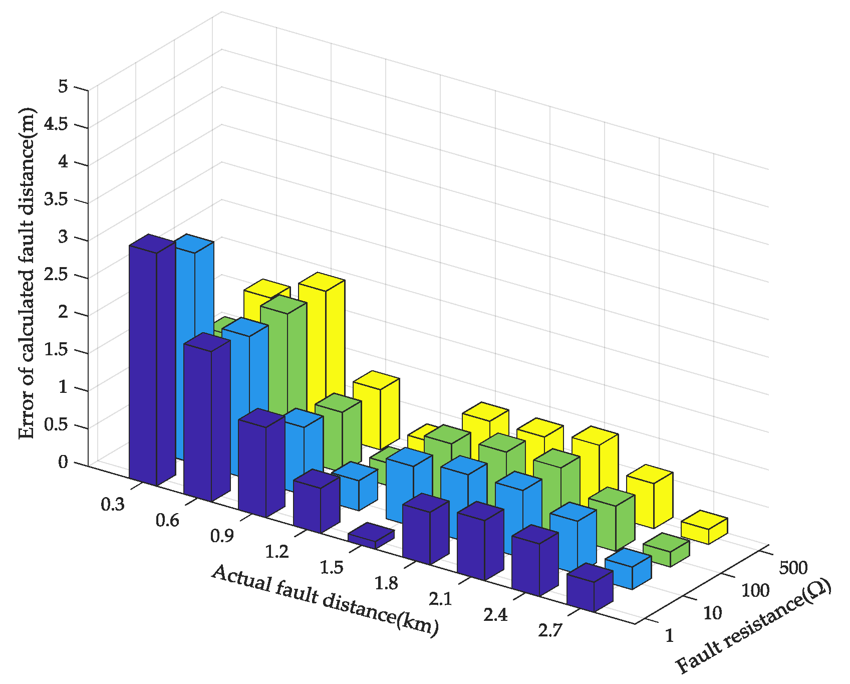
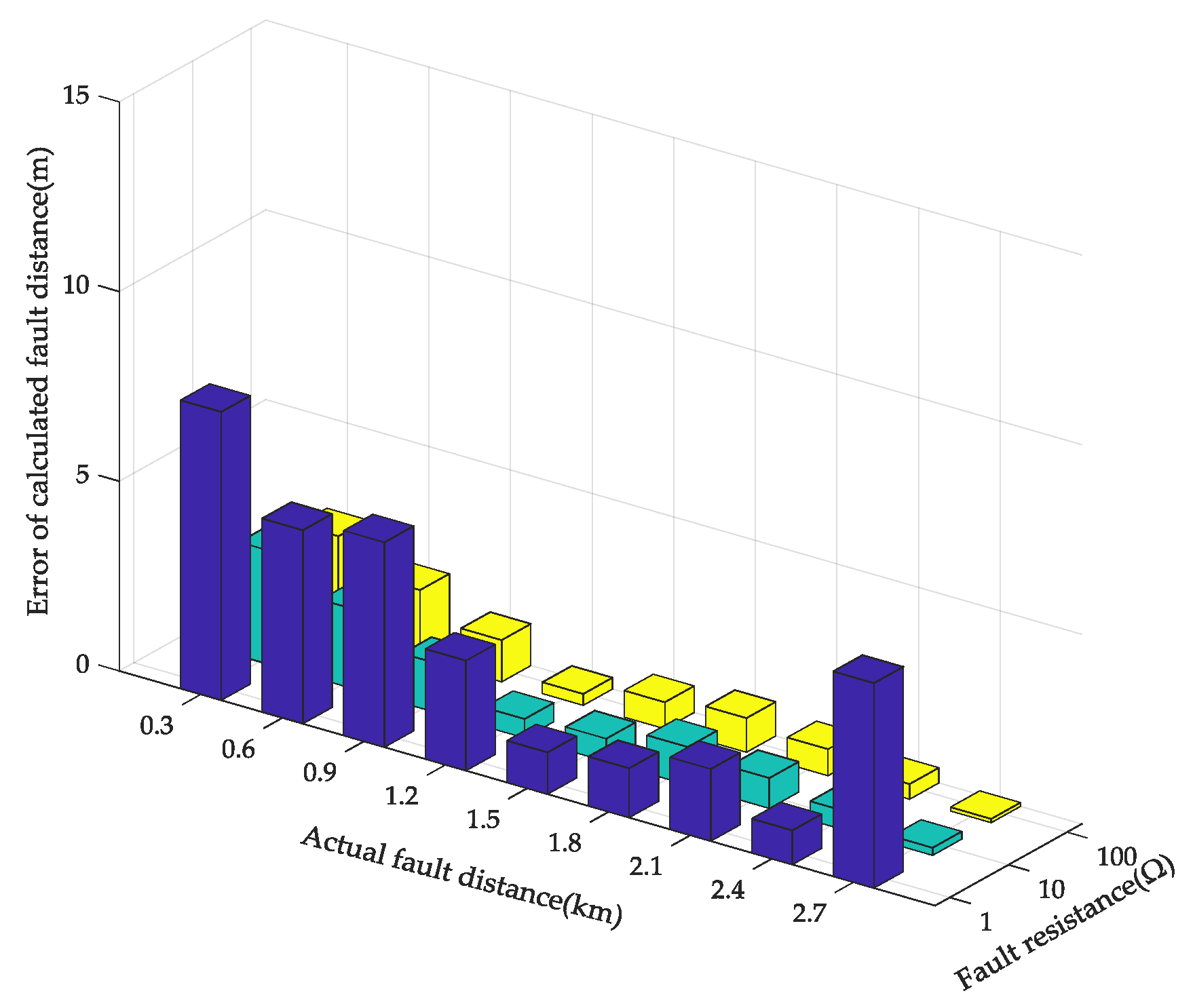
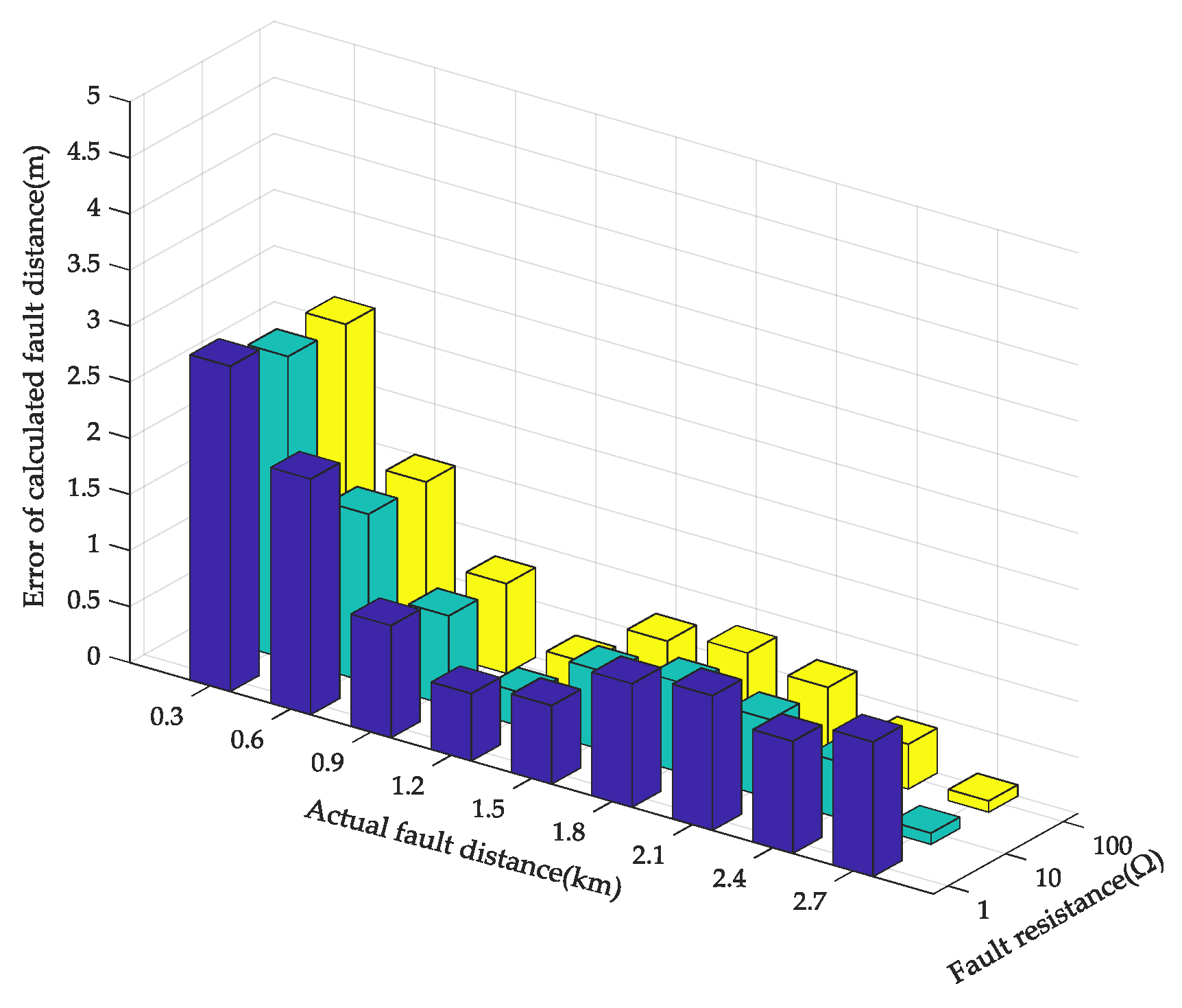
All simulation tests indicated that the results of the fault location were accurate. Due to space limitations, traversal simulation results of fault location for section PT in three-terminal line are listed as Figure 5, Figure 6 and Figure 7 to show the general performance of the algorithm. The representative and specific calculation results are listed in

Table 2. Partial calculated results of the fault location in a three-terminal line.

Faulty Section	Fault Distance (km)	Fault Type	Fault Resistance (Ω)	Calculated Results
				Faulty Section	Fault Distance (km)	Error of Fault Distance (m)
MT	0.2	a-g	1	MT	0.1967	3.3
			10	MT	0.1969	3.1
			100	MT	0.1965	3.5
			500	MT	0.1961	3.9
		a-b-g	1	MT	0.1968	3.2
			10	MT	0.1978	2.2
			100	MT	0.1984	1.6
		a-b	1	MT	0.1972	2.8
			10	MT	0.1983	1.7
			100	MT	0.1985	1.5
NT	1.5	a-g	1	NT	1.4991	0.9
			10	NT	1.4991	0.9
			100	NT	1.4991	0.9
			500	NT	1.4980	2
		a-b-g	1	NT	1.5004	0.4
			10	NT	1.4991	0.9
			100	NT	1.4986	1.4
		a-b	1	NT	1.4975	2.5
			10	NT	1.4988	1.2
			100	NT	1.4988	1.2
TP	2.5	a-g	1	PT	2.4993	0.7
			10	PT	2.4994	0.6
			100	PT	2.4995	0.5
			500	PT	2.4995	0.5
		a-b-g	1	PT	2.5001	0.1
			10	PT	2.4998	0.2
			100	PT	2.4997	0.3
		a-b	1	PT	2.4991	0.9
			10	PT	2.4996	0.4
			100	PT	2.4997	0.3

,

Table 3. The results of fault location when the fault occurs near the tapping point.

Faulty Section	Distance between Point F and T (m)	Fault Type	Fault Resistance (Ω)	Calculated Results
				Faulty Section	Distance between Point F and T (km)	Error of Fault Distance (m)
MT	10	a-g	1	MT	10.8	0.8
			10	MT	10.9	0.9
			100	MT	10.9	0.9
			500	MT	10.7	0.7
NT	20	a-b-g	1	NT	19.0	1.0
			10	NT	19.5	0.5
			100	NT	19.5	0.5
TP	30	a-b	1	PT	30.3	0.3
			10	PT	29.8	0.2
			100	PT	29.7	0.3

and

Table 4. The calculated line parameters for typical fault conditions.

Faulty Section	Fault Distance (km)	Fault Type	Fault Resistance (Ω)	Solved Results		Error of ${\mathit{r}}_{\mathbf{s}1}$ (%)	Error of ${\mathit{l}}_{\mathbf{s}1}$ (%)	Error of ${\mathit{r}}_{\mathbf{m}1}$ (%)	Error $\mathbf{of} {\mathit{l}}_{\mathbf{m}1}$ (%)
				${\mathit{z}}_{\mathbf{s}1}$ (Ω/km)	${\mathit{z}}_{\mathbf{m}1}$ (Ω/km)
MT	0.2	a-g	1	0.2385 + j1.0487	0.0370 + j0.4697	4.01	3.55	4.82	3.53
			10	0.2384 + j1.0487	0.0369 + j0.4697	3.97	3.55	4.53	3.53
			100	0.2383 + j1.0487	0.0369 + j0.4697	3.92	3.55	4.53	3.53
NT	1.5	a-b-g	1	0.2375 + j1.0490	0.0368 + j0.4695	3.58	3.58	4.25	3.48
			10	0.2371 + j1.0489	0.0363 + j0.4697	3.40	3.57	2.83	3.53
			100	0.2369 + j1.0489	0.0362 + j0.4697	3.31	3.57	2.55	3.53
PT	2.5	a-b	1	0.2387 + j1.0478	0.0366 + j0.4687	4.10	3.47	3.68	3.31
			10	0.2389 + j1.0481	0.0369 + j0.4690	4.19	3.50	4.53	3.37
			100	0.2389 + j1.0481	0.0368 + j0.4690	4.19	3.50	4.25	3.37

for detailed analysis. Given the similarity between the three-terminal line model and tapped line model, only partial results of the fault location in the tapped line model are listed in

Table 5. Partial calculated results of the fault location in a tapped line.

Faulty Section	Fault Distance (km)	Fault Type	Fault Resistance (Ω)	Solved Results		Error of Fault Distance (m)
				Faulty Section	Fault Distance (km)
MT	0.2	a-g	1	MT	0.1974	2.6
			10	MT	0.1947	5.3
			100	MT	0.1941	5.9
NT	1.5	a-b-g	1	NT	1.4990	1
			10	NT	1.4993	0.7
			100	NT	1.4993	0.7
PT	2.5	a-b	1	PT	2.4997	0.3
			10	PT	2.4998	0.2
			100	PT	2.4998	0.2

to verify the effectiveness of algorithm in tapped line.

In this paper, the error of distance calculation is defined as in Equation (28):

$$Erro{r}_L=\left|L_{actual}-L_{calculated}\right|$$

(28)

The error of line parameter calculation is expressed as in Equation (29):

$$Erro{r}_z=\left|\frac{Z_{actual}-Z_{calculated}}{Z_{actual}}\right|\times 100\%$$

(29)

3.2.1. Effect of the Fault Position

Figure 5, Figure 6 and Figure 7 show the errors of the computed fault distances with the change of fault position and fault resistance when an a-g, a-b-g, or a-b fault occurs on section PT, respectively. Table 2 also lists the specific results of the fault location in the typical fault positions. The results have a very small difference between them and their errors are all within 10 m.

In addition, research was conducted in order to verify the validity of this algorithm on the condition that the fault occurs near the tapping point. The simulation results listed in Table 3 show that the obtained fault location results are still accurate.

These results reveal the immunity of the proposed algorithm against the fault position.

3.2.2. Effect of the Fault Resistance

Table 2 summarizes the computed fault distances under 1, 10, 100, 500 Ω fault resistance, indicating that the errors in most cases were no more than 5 m. Actually, the fault location equations do not involve the fault resistance, so the relationship between the various electrical quantities in the equations is not affected by fault resistance in principle. The results show that the algorithm was basically independent of fault resistance.

3.2.3. Effect of an Unbalanced Fault Type

The fault scenarios considering various unbalanced fault types were tested, such as single-phase earth fault, two-phase earth fault, and two-phase short circuit fault. The calculated results are presented in Table 2. The errors within 5 m indicate that the proposed algorithm displayed good performance irrespective of the unbalanced fault type.

3.2.4. Effect of the Line Parameter

The proposed fault location algorithm takes the line parameter as unknown by-products to be solved without requiring line parameter as inputs. The calculated line parameters of line MN when the fault occurred 1 km away from terminal M on section MT are shown in Table 4. Compared with the true line parameter values per unit length, as in Equation (30), the maximum error of the calculated parameter values was less than 5%, showing the high accuracy.

$$\begin{gathered} z_{\mathrm{s}1}=\left(z_{\mathrm{mn}0}+2\times z_{\mathrm{mn}1}\right)/3=0.2293+\mathrm{j}1.0127 \left(\mathrm{\Omega }/\mathrm{km}\right) \\ {z}_{\mathrm{m}1}=\left(z_{\mathrm{mn}0}-z_{\mathrm{mn}1}\right)/3=0.0353+\mathrm{j}0.4537 \left(\mathrm{\Omega }/\mathrm{km}\right) \\ {z}_{\mathrm{s}2}=\left(z_{\mathrm{tp}0}+2\times z_{\mathrm{tp}1}\right)/3=0.382+\mathrm{j}0.7533 \left(\mathrm{\Omega }/\mathrm{km}\right) \\ {z}_{\mathrm{m}2}=\left(z_{\mathrm{tp}0}-z_{\mathrm{tp}1}\right)/3=0.05+\mathrm{j}0.3453 \left(\mathrm{\Omega }/\mathrm{km}\right) \end{gathered}$$

(30)

Therefore, when data errors do not exist, the proposed algorithm has a high accuracy and is basically affected by fault position, fault resistance, unbalanced fault type, and line parameter in three-terminal line. The same simulations were also performed in a tapped line, and the partial calculated results are listed in Table 5, which also show good performance and reveal the effectiveness of the algorithm in a tapped line.

3.3. Performance of the Fault Location Algorithm Considering Data Error

Considering the usual ±1% data error due to measurement, background noise, and fundamental component calculation in distribution network [22,23], the accuracy of the proposed algorithm in this case is evaluated in this section.

Thirty sets of three-terminal post-fault sampling data were obtained using Simulink, and the corresponding fundamental voltages and currents were extracted using a DFT algorithm in the three-terminal line model. Furthermore, ±1% Gaussian white noise was added to each fundamental component to simulate the ±1% data error. Then, the fault location algorithm was conducted in MATLAB. Because of the randomness of Gaussian white noise, the result of one test could not effectively explain the performance of the algorithm. Thus, tests were carried out 20 times for each fault condition.

First, only one set of sampling data was used in the algorithm and

Table 6. The statistical results of the fault location in the case of ±1% data error.

Faulty Section	Fault Distance (km)	Fault Resistance (Ω)	Fault Type	Results from One Set of Data			Results from 30 Sets of Data
				The Number of Errors within This Range		Failure	The Number of Errors within This Range
				0–100 (m)	>100 (m)		0–50 (m)	50–100 (m)	>100 (m)
MT	0.5	1	a-g	6	12	2	18	2	0
		10	a-b-g	4	16	0	20	0	0
		100	a-b	7	12	1	18	2	0
PT	1	1	a-g	6	12	2	16	3	1
		10	a-b-g	8	9	3	18	2	0
		100	a-b	7	12	1	17	3	0

presents the statistical results. When the a-g fault with a 1 Ω fault resistance occurred at 0.5 km away from M on section MT, the tests for the fault location were conducted 20 times, but only 6 tests gave the results with errors in 0–100 m range, and the result errors of 12 tests were greater than 100 m. Specifically, this algorithm failed twice. In general, the algorithm yielded the results with errors greater than 100 m in most cases and the average error was about 146 m. Furthermore, the algorithm sometimes failed to give the results.

Then, 30 sets of sampling data were used to locate the fault. By contrast, most of the result errors were within 0–50 m and the average error was about 36 m. There was no failure in any of the tests. It can be seen that the improved algorithm could give the location results reliably and has high accuracy.

The same research was carried out in a tapped line model and the proposed improved algorithm also displayed good performance. Therefore, the fault location algorithm using 30 sampled windows could resist the influence of the data error to some extent and had a better performance than using one sampled window.

4. Conclusions

In view of the influence of line parameters on the conventional algorithm, this paper proposes a parameter-free fault location algorithm for a T-type transmission line in a distribution network with neutral grounding via low resistance. When the line parameters are unknown, this algorithm can identify the faulty branch and find the fault distance only using the post-fault redundant synchronous measurements of three terminals and the length of lines. This algorithm is basically unaffected by fault position, unbalanced fault type, fault resistance, line parameter, and data error. Its accuracy and robustness have been verified using the simulation results. This algorithm is also suitable for the short T-type overhead lines in a transmission network when the three-terminal synchronous post-fault measurements can be obtained. The main contributions of the proposed fault location algorithm are as follows:

• The line parameter values are not required because they are taken as unknowns to solve together with the fault distance.
• The influence of data error can be resisted to some extent based on the redundant data and estimation theory.
• The high reliability and robustness can be ensured via the use of a trust-region algorithm to solve the non-linear equations.
• The fault point can be identified directly according to the reasonability of the equations’ solutions, avoiding a series of problems when the faulty section judgment is performed first in most indirect methods.

Research of the parameter-free fault location method, which is applicable to the distributed parameter line model, is our next focus.

References

- Mahamedi, B.; Sanaye-Pasand, M.; Azizi, S.; Zhu, J.G. Unsynchronised fault-location technique for three-terminal lines. IET Gen. Transm. Distrib. 2015, 9, 2099–2107. [Google Scholar] [CrossRef]
- Evrenosoglu, C.Y.; Abur, A. Travelling wave based fault location for teed circuits. IEEE Trans. Power Deliv. 2005, 20, 1115–1121. [Google Scholar] [CrossRef]
- Niazy, I.; Sadeh, J. A new single ended fault location algorithm for combined transmission line considering fault clearing transients without using line parameters. Int. J. Electr. Power Energy Syst. 2013, 44, 816–823. [Google Scholar] [CrossRef]
- Livani, H.; Evrenosoglu, C.Y. A Fault Classification and Localization Method for Three-Terminal Circuits Using Machine Learning. IEEE Trans. Power Deliv. 2013, 28, 2282–2290. [Google Scholar] [CrossRef]
- Ahmadimanesh, A.; Shahrtash, S.M. Transient-Based Fault-Location Method for Multiterminal Lines Employing S-Transform. IEEE Trans. Power Deliv. 2013, 28, 1373–1380. [Google Scholar] [CrossRef]
- De Pereira, C.E.M.; Zanetta, L.C., Jr. Fault Location in Multitapped Transmission Lines Using Unsynchronized Data and Superposition Theorem. IEEE Trans. Power Deliv. 2011, 26, 2081–2089. [Google Scholar] [CrossRef]
- Elsadd, M.A.; Abdelaziz, A.Y. Unsynchronized fault-location technique for two- and three-terminal transmission lines. Electr. Power Syst. Res. 2018, 158, 228–239. [Google Scholar] [CrossRef]
- Gao, H.L.; An, Y.Q.; Jiang, S.F. Study on accurate fault location algorithm for EHV teed lines. Autom. Electr. Power Syst. 2001, 25, 51–54. [Google Scholar]
- Gaur, V.K.; Bhalja, B. A new faulty section identification and fault localization technique for three-terminal transmission line. Int. J. Electr. Power Energy Syst. 2017, 93, 216–227. [Google Scholar] [CrossRef]
- Lin, Y.H.; Liu, C.W.; Yu, C.S. A new fault locator for three-terminal transmission lines using two-terminal synchronized voltage and current phasors. IEEE Trans. Power Deliv. 2002, 17, 452–459. [Google Scholar] [CrossRef]
- Lin, T.C.; Lin, P.Y.; Liu, C.W. An Algorithm for Locating Faults in Three-Terminal Multisection Nonhomogeneous Transmission Lines Using Synchrophasor Measurements. IEEE Trans. Smart Grid 2014, 5, 38–50. [Google Scholar] [CrossRef]
- Girgis, A.A.; Hart, D.G.; Peterson, W.L. A new fault location technique for two- and three-terminal lines. IEEE Trans. Power Deliv. 1992, 7, 98–107. [Google Scholar] [CrossRef]
- Izykowski, J.; Rosolowski, E.; Saha, M.M.; Fulczyk, M.; Balcerek, P. A Fault-Location Method for Application with Current Differential Relays of Three-Terminal Lines. IEEE Trans. Power Deliv. 2007, 22, 2099–2107. [Google Scholar] [CrossRef]
- Shi, S.H.; He, B.T.; Zhang, W.J. Fault location for HV three-terminal transmission. Proc. CSEE 2008, 28, 105–110. [Google Scholar]
- Al-Mohammed, A.H.; Abido, M.A. An adaptive fault location algorithm for power system networks based on synchrophasor measurements. Electr. Power Syst. Res. 2014, 108, 153–163. [Google Scholar] [CrossRef]
- Davoudi, M.; Sadeh, J.; Kamyab, E. Transient-Based Fault Location on Three-Terminal and Tapped Transmission Lines Not Requiring Line Parameters. IEEE Trans. Power Deliv. 2018, 33, 179–188. [Google Scholar] [CrossRef]
- Affijulla, S.; Tripathy, P. Development of Phasor Estimation Algorithm for P-Class PMU Suitable in Protection Applications. IEEE Trans. Smart Grid 2018, 9, 1250–1260. [Google Scholar] [CrossRef]
- Pignati, M.; Zanni, L.; Romano, P.; Cherkaoui, R.; Paolone, M. Fault Detection and Faulted Line Identification in Active Distribution Networks Using Synchrophasors-Based Real-Time State Estimation. IEEE Trans. Power Deliv. 2018, 32, 381–392. [Google Scholar] [CrossRef]
- Asprou, M.; Kyriakides, E. Identification and Estimation of Erroneous Transmission Line Parameters Using PMU Measurements. IEEE Trans. Power Deliv. 2017, 32, 2510–2519. [Google Scholar] [CrossRef]
- Ramamoorty, M. Application of digital computers to power system protection. J. Inst. Eng. 1972, 52, 235–238. [Google Scholar]
- Abdelaziz, M.M.A.; Farag, H.E.; El-Saadany, E.F.; Mohamed, Y.A.I. A Novel and Generalized Three-Phase Power Flow Algorithm for Islanded Microgrids Using a Newton Trust Region Method. IEEE Trans. Power Syst. 2013, 28, 190–201. [Google Scholar] [CrossRef]
- Zhang, S.; Lin, S.; He, Z.; Lee, W. Ground fault location in radial distribution networks involving distributed voltage measurement. IET Gen. Transm. Distrib. 2018, 12, 987–996. [Google Scholar] [CrossRef]
- Von Meier, A.; Stewart, E.; McEachern, A.; Andersen, M.; Mehrmanesh, L. Precision Micro-Synchrophasors for Distribution Systems: A Summary of Applications. IEEE Trans. Smart Grid 2017, 8, 2926–2936. [Google Scholar] [CrossRef]
Figure 1.
T-type transmission line structure.
Figure 2.
The mode of constructing data window.
Figure 3.
Flowchart of solving by trust-region algorithm.
Figure 4.
Algorithm flow chart.
Figure 5.
Error of computed fault distance for a-g fault on PT section.
Figure 6.
Error of computed fault distance for a-b-g fault on PT section.
Figure 7.
Error of computed fault distance for a-b fault on the PT section.