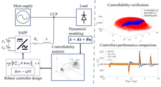
Robust Control of Shunt Active Power Filters: A Dynamical Model-Based Approach with Verified Controllability

Abstract

This paper presents the robust control of Three-Leg Split-Capacitor Shunt Active Power Filters (TLSC SAPFs) by means of structured $H\infty$ controllers for reactive, unbalanced, and harmonic compensation and the DC-link bus voltage regulation. Robust controller synthesis is performed based on the TLSC SAPF dynamical model including power losses in passive elements. Before the control implementation, a systematic procedure for the nonlinear controllability verification of the converter and its quantification using the set-theoretic approach is presented. Controllability verification serves to accurately design the SAPF’s operation region. Thus, a Voltage Oriented Control (VOC) structure is implemented by using two different approaches to determine the PI controller parameters: (1) the traditional Pole-Placement method (PP-PI) and (2) the $H\infty$-PI structured synthesis approach, which leads to PI robust controllers. From the latter approach, two sets of parameters are obtained. The first set considers the nominal model ($H\infty$-PI), and the second one explicitly accounts for the model parametric uncertainties ($H\infty$-uPI). An optimization procedure is presented for obtaining the optimal $H\infty$-PI and $H\infty$-uPI controller parameters where four complementary constrains are defined to establish a trade-off between the controllers performance and robustness. The enforcement of constraints is later evaluated for each of three PI controllers obtained. This work aims to establish a common ground for the comparison of robust control strategies applied to TLSC APFs; therefore, the TLSC SAPF compensation performance is measured and compared with the performance indices: integral of the absolute error ($IAE$), integral of the time-weighted absolute error ($ITAE$), integral of the absolute control action ($IUA$), and maximum sensitivity ($M_s$).

1. Introduction

In three-phase four-wire power systems, the proliferation of inefficient loads causes undesired reactive power demand, harmonic distortion, and unbalanced currents. Consequently, users and utilities must face excessive power losses in electric networks, the most representative being wire [1,2] and transformer [3,4] losses. Another drawback of power systems with the presence of inefficient power is the circulation of neutral currents that worsen power quality and lead to technical problems [5]. Shunt Active Power Filters (SAPFs) are often used for mitigating these problems. SAPFs are connected in parallel with loads and compensate the currents related to the inefficient power. Such compensation avoids the circulation of inefficient currents in power systems, reducing power losses, increasing the overall system efficiency, and improving power quality of the system.

The Three-Leg Split-Capacitor (TLSC) SAPF is one of the most common devices used in the industry for compensating inefficient currents [6,7]. The research community also recommends the use of the TLSC SAPF topology; after a comprehensive study of SAPF topologies, the authors in [8] concluded that TLSC SAPF features a superior performance over other SAPF topologies for low-to-medium-power applications, providing satisfactory results under both steady-state and dynamic performance conditions. The TLSC SAPF topology has only three legs, which facilitates the implementation of any control strategy, each of its legs being independently controlled. Concerning the split capacitor, it gives the possibility of controlling zero-sequence currents produced by unbalanced and third harmonic currents. For the aforementioned reasons, in this paper, TLSC SAPF is selected for the design of a robust control structure with verified controllability.

For improving the dynamic behavior of TLSC SAPF, researchers have focused on implementing advanced control techniques. To mention some of the most relevant and recently published papers: Reference [9] implemented a current controller based on particle swarm optimization for correcting the steady-state error. Reference [10] proposed a robust repetitive controller for following voltage and current signals, achieving zero steady-state errors. Reference [11] suppressed the low frequency harmonics whose frequencies are lower than the resonance frequency and mitigated the rest of the harmonics by a resonance damping method. In [12], a modified passivity-based control was proposed for handling steady-state current error where an error proportional-integral regulator was inserted into the coupling loop. Reference [13] proposed a parallel resonance detection and control scheme, which includes square-wave current active injection and selective compensation with closed-loop regulation. Reference [14] presented a control strategy that includes an algorithm for a proper selective compensation for inefficient load currents when power capacity in SAPF is exceeded. Although numerous papers have been reported concerning advanced control techniques for SAPF, as can be seen from the bibliographic search, most of the research is focused on obtaining a better performance of the closed-loop system. Moreover, one of the most widely adopted controllers that remains as the standard for power electronic converters is the PI controller. This is due to its ease of implementation and good performance in most applications (provided that it is properly tuned). Furthermore, there are plenty of techniques to compute its parameters [15]. Notwithstanding that the PI controller would be one of main players in the power electronics field to automatically regulate most of the converters, it has been recently reported in the literature as a general rule that only about one third of the PI/PID-based control loops works properly, and one third has poorly tuned controllers [16]. This makes the tuning of PI/PID controllers a very active and still relevant research topic.

The main contribution of this paper is the robust control synthesis of PI controllers for SAPFs by using $H\infty$ controllers and taking into account the model parameters’ uncertainty. Basically, our paper proposes the use of a state-of-the-art technique for synthesizing robust PI controllers to the SAPF that achieves high standards in the stabilization of the closed-loop system with guaranteed performance. This technique leads to the optimization of the PI controllers instead of the classical tuning approximation [17,18]. The design of PI/PID controllers that are robust in the presence of system uncertainty is a recurrent challenge in control engineering due to the inevitable mismatch between the real device and its mathematical model [18]. Nevertheless, this problem can be intrinsically handled by means of a structured $H\infty$-control design [19]. Despite the fact that neither the application of $H\infty$ optimization-based controllers, nor the idea of structured $H\infty$-PI controllers’ synthesis are new in the power electronics converters field (see, e.g., [20,21] for some $H\infty$ applications and [22] for structured $H\infty$-PI controllers), to the best of the authors’ knowledge, this approach has not been yet applied to the control of three-phase four-wire active filters such as TLSC SAPFs.

The dynamical performance of a closed-loop control system highly depends on the controllability of the system that we want to control. Increasing system controllability leads to a better closed-loop system response [23]. Controllability is concerned with the ability of the system to be driven from an initial state to a desired one by applying a control input sequence [24]. Researchers frequently perform the controllability analysis of DC–DC converters after linearizing the dynamical model by means of Kalman’s rank condition [24]. Generally, controllability is a property of power electronic converters that is given as granted. However, the authors in [25] recently proved that a DC-DC converter is controllable only if certain conditions are met, and that is a property that could change depending on the region in which the system is operated. For power electronics devices that have an inherent non-linear behavior, it is more convenient to use Lie’s brackets method [25]. The evaluation of the controllability by using both the rank of the controllability matrix for linear systems and Lie’s brackets method for non-linear systems allows verifying if the system is controllable or not; nonetheless, such techniques do not permit its quantification. To overcome this limitation, the controllability analysis via the set-theoretic approach has been applied by some authors [26,27,28]. This approach allows not only the system controllability verification, but also its quantification. Furthermore, in [29], it was shown that the controllability verifications via the set-theoretic approach and Lie’s brackets method are equivalent. Consequently, the controllability analysis based on the set-theoretic approach as proposed by the authors in [30] is adopted in this work to verify whether the designed TLSC SAPF is controllable. Additionally, a normalized controllability index ($CI$) is introduced as proposed in [27] for quantifying SAPF controllability. This controllability analysis is performed here to support the validity of the designed robust PI controllers in a wide region around the nominal operation point. A $CI$ close to one will indicate a highly controllable system, then the closed-loop control system performance will depend mainly on the selected control structure and its parameters’ synthesis method. This is of foremost importance because it permits establishing a benchmark to evaluate either new PI/PID controller synthesis methods or other control structures applied to the TLSC SAPF.

This paper is composed of the following sections: Section 2 presents the TLSC SAPF dynamical modeling in the $dq0$ frame. Section 3 describes the robust control structure design, performance indices, and controllability index. Section 4 presents the results, which include: the evaluation of the controllability of the system, the computation of the $CI$, controllers synthesis, the computation of performance indices, and the evaluation of compensation performance. Finally, Section 5 concludes and highlights the most relevant aspects of this paper.

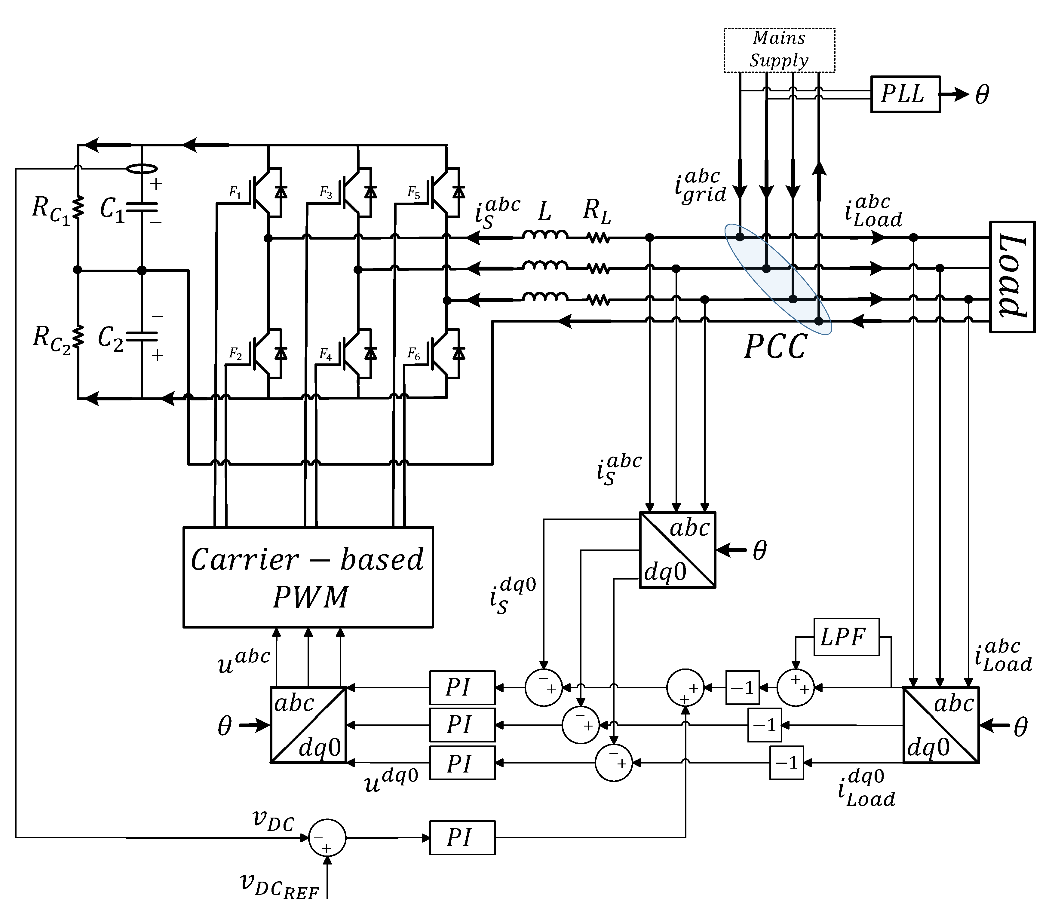
2. TLSC SAPF Dynamical Modeling

The TLSC SAPF under study is depicted in Figure 1. It is mainly composed of a split-capacitor DC-link ($C_1$ and $C_2$) and a three-phase Voltage Source Inverter (VSI). The TLSC SAPF is connected in parallel at the Point of Common Coupling (PCC) through an L filter, and its function is to compensate the inefficient currents generated in the load, avoiding their circulation through the main supply. The neutral wire is directly connected to the mid-point of the DC link as presented by [31,32,33,34] to mitigate zero sequence currents produced by non-linear and unbalanced load components. Resistors $R_{C_1}$, $R_{C_2}$, and $R_L$ represent the converter losses, which reflect a more realistic approximation of the system.

Equation (1) corresponds to the switching function $u^{abc}$ for activating power switches $F_{1,2,3,4,5,6}$ of the VSI. Assuming that switches $F_{1,3,5}$ and $F_{2,4,6}$ are complementary:

$$\begin{array}{ccc}\hfill u^{abc}& =& \left\{\begin{array}{ccccc}1\hfill & \mathrm{if}\hfill & F_{1,3,5}=on\hfill & \mathrm{and}\hfill & F_{2,4,6}=off\hfill \\ -1\hfill & \mathrm{if}\hfill & F_{1,3,5}=off\hfill & \mathrm{and}\hfill & F_{2,4,6}=on\hfill \end{array}\right.\hfill \end{array}$$

(1)

$u^{abc}$ in terms of $F_{1,3,5}$ and $F_{2,4,6}$ are given by Equations (2) and (3), respectively.

$$\begin{array}{ccc}\hfill u^{abc}& =& 2F_{1,3,5}-1\hfill \end{array}$$

(2)

$$\begin{array}{ccc}\hfill u^{abc}& =& 1-2F_{2,4,6}\hfill \end{array}$$

(3)

By applying Kirchhoff’s laws to the system in Figure 1, the large-signal dynamical model of the converter is given by:

$$\begin{array}{ccc}\hfill L{\displaystyle \frac{d{i}_S^{abc}}{dt}}& =& -R_L{i}_S^{abc}-{\displaystyle \frac{v_{DC}}{2}}{u}^{abc}-{\epsilon }_v+v_{pcc}^{abc}\hfill \\ \hfill C{\displaystyle \frac{d{v}_{DC}}{dt}}& =& i_S^{abc}{u}^{ab{c}^T}-{\displaystyle \frac{v_{DC}}{R_o}}\hfill \\ \hfill 2C{\displaystyle \frac{d{\epsilon }_v}{dt}}& =& i_S^{abc}-{\displaystyle \frac{2{\epsilon }_v}{R_o}}\hfill \end{array}$$

(4)

where $v_{DC}=v_{C_1}-v_{C_2}$ is the total DC voltage, $2{\epsilon }_v=v_{C_1}+v_{C_2}$ is the differential DC voltage between capacitors $C_1$ and $C_2$, $C_1=C_2=C$, and $R_{C_1}=R_{C_2}=R_o$.

It is well known that the model given by the equations in (4) describes the system evolution in terms of sinusoidal signals, which are not the most appropriate to perform the design and control tasks [35]. Consequently, $dq0$ transformation is applied to decompose the $abc$ system into its direct, quadrature, and zero sequence components (Equation (5)) [36]. The direct component is denoted by subscript d and is associated with the active power component; the quadrature component is denoted by subscript q and is associated with the reactive power component; and the zero sequence component is denoted by subscript 0 and contains harmonics and unbalanced components. After $dq0$ transformation, the TLSC SAPF model becomes:

$$\begin{array}{ccc}\hfill L\left[\left[\begin{array}{c}-\omega i_S^q\\ \omega i_S^d\\ 0\end{array}\right]+{\displaystyle \frac{d{i}_S^{dq0}}{dt}}\right]& =& -R_L{i}_S^{dq0}-{\displaystyle \frac{v_{DC}}{2}}{u}^{dq0}-\left[\begin{array}{c}0\\ 0\\ \sqrt{3}\end{array}\right]{\epsilon }_v+v_{pcc}^{dq0}\hfill \\ \hfill C{\displaystyle \frac{d{v}_{DC}}{dt}}& =& i_S^{dq0}{u}^{dq{0}^T}-{\displaystyle \frac{v_{DC}}{R_o}}\hfill \\ \hfill 2C{\displaystyle \frac{d{\epsilon }_v}{dt}}& =& \sqrt{3}{i}_S^0-{\displaystyle \frac{2{\epsilon }_v}{R_o}}\hfill \end{array}$$

(5)

where $\omega$ is the AC angular frequency; while $i_S^{dq0}$, $v_{pcc}^{dq0}$, and $u^{dq{0}^T}$ are currents, voltages, and switching functions in the $dq0$ frame; respectively.

For a balanced source and load, the $dq$ components in Model (5) reach a constant value when the system is in a steady-state condition, while the zero sequence is equal to zero. In contrast, for unbalanced loads, the $dq0$ components are composed of a constant quantity plus a small oscillatory part with twice the nominal grid frequency [37]. Furthermore, in the presence of harmonic loads, the $dq0$ components have other oscillatory components that depend on the order of the current harmonics [38].

From the large-signal model given by the equations in (5), the TLSC SAPF small-signal model is obtained by applying the following standard state-space realization:

$$\begin{array}{ccc}\hfill \dot{\mathbf{x}}& =& \mathbf{A}\mathbf{x}+\mathbf{B}\mathbf{u}\hfill \\ \hfill \mathbf{y}& =& \mathbf{C}\mathbf{x}+\mathbf{D}\mathbf{u}\hfill \end{array}$$

(6)

with:

$$\begin{array}{c}\hfill \mathbf{A}={\left({\displaystyle \frac{\partial f\left(\mathbf{x},\mathbf{u}\right)}{\partial x_i}}\right)}_{{\mathbf{x}}_e,{\mathbf{u}}_e}\mathbf{B}={\left({\displaystyle \frac{\partial f\left(\mathbf{x},\mathbf{u}\right)}{\partial u_i}}\right)}_{{\mathbf{x}}_e,{\mathbf{u}}_e}\\ & & \\ \hfill \mathbf{C}={\left({\displaystyle \frac{\partial h\left(\mathbf{x},\mathbf{u}\right)}{\partial x_i}}\right)}_{{\mathbf{x}}_e,{\mathbf{u}}_e}\mathbf{D}={\left({\displaystyle \frac{\partial h\left(\mathbf{x},\mathbf{u}\right)}{\partial u_i}}\right)}_{{\mathbf{x}}_e,{\mathbf{u}}_e}\end{array}$$

(7)

where $x_i$ refers to the ith state variable, $f(x,u)$ refers to each equation of Model (5), and $h(x,u)$ refers to the equations that relate state and output variables, in this paper $h(x,u)=x$. Subscript e in (7) refers to both state variables ($x_e$) and input variables ($u_e$) in their rated values, which are represented with capital letters in Equations (8)–(15).

In this modeling stage and for obtaining the A, B, C, and D matrices, state variables are defined as $\mathbf{x}={\left[i_S^d,i_S^q,i_S^0,v_{DC},{\epsilon }_v\right]}^T$; input variables are defined as $\mathbf{u}={\left[u^d,u^q,u^0,v_{pcc}^d,v_{pcc}^q,v_{pcc}^0\right]}^T$; and output variables are defined as equal to the state variables as $\mathbf{y}=\mathbf{x}$$={\left[i_S^d,i_S^q,i_S^0,v_{DC},{\epsilon }_v\right]}^T$.

Due to the fact that for a balanced load, the zero sequence components become zero, i.e., $v_{pcc}^0=0$, $i_S^0=0$, and $u^0=0$, thus the coupling between the $dq$ and zero components can be neglected, and the TLSC SAPF $dq0$ small-signal model can be split into: (i.) a TLSC SAPF $dq$ small-signal and (ii.) a TLSC SAPF 0 sequence small-signal model, respectively, as follows:

$$\begin{array}{ccc}\hfill \left[\begin{array}{c}{\dot{i}}_L^d\\ {\dot{i}}_L^q\\ {\dot{v}}_{DC}\end{array}\right]& =& \left[\begin{array}{ccc}-{\displaystyle \frac{R_L}{L}}& \omega & -{\displaystyle \frac{U^d}{2L}}\\ \\ -\omega & -{\displaystyle \frac{R_L}{L}}& -{\displaystyle \frac{U^q}{2L}}\\ \\ {\displaystyle \frac{U^d}{C}}& {\displaystyle \frac{U^q}{C}}& -{\displaystyle \frac{1}{R_{o}C}}\end{array}\right]\left[\begin{array}{c}{i}_S^d\\ i_S^q\\ v_{DC}\end{array}\right]+\left[\begin{array}{cccc}-{\displaystyle \frac{V_{DC}}{2L}}& 0& {\displaystyle \frac{1}{L}}& 0\\ \\ 0& -{\displaystyle \frac{V_{DC}}{L}}& 0& {\displaystyle \frac{1}{L}}\\ \\ {\displaystyle \frac{I_S^d}{C}}& {\displaystyle \frac{I_S^q}{C}}& 0& 0\end{array}\right]\left[\begin{array}{c}{u}^d\\ u^q\\ v_{pcc}^d\\ v_{pcc}^q\end{array}\right]\hfill \end{array}$$

(8)

$$\begin{array}{ccc}\hfill \left[\begin{array}{c}{\dot{i}}_L^0\\ {\dot{\epsilon }}_v\end{array}\right]& =& \left[\begin{array}{cc}-{\displaystyle \frac{R_L}{L}}& -{\displaystyle \frac{\sqrt{3}}{L}}\\ \\ {\displaystyle \frac{\sqrt{3}}{2C}}& -{\displaystyle \frac{1}{R_{o}C}}\end{array}\right]\left[\begin{array}{c}{i}_S^0\\ {\epsilon }_v\end{array}\right]+\left[\begin{array}{cc}-{\displaystyle \frac{V_{DC}}{L}}& {\displaystyle \frac{1}{L}}\\ \\ 0& 0\end{array}\right]\left[\begin{array}{c}{u}^0\\ v_{pcc}^0\end{array}\right]\hfill \end{array}$$

(9)

If the system states are taken as the system outputs, matrix $\mathbf{C}$ corresponds to a $3\times 3$ identity matrix for the model given by Equation (8) while a $2\times 2$ identity matrix for the model given by Equation (9). On the other hand, matrix $\mathbf{D}$ is a $4\times 3$ matrix of zeros and a $2\times 2$ matrix of zeros for models given by Equations (8) and (9), respectively.

Note that the converter small-signal model given by Equation (8) is in the time domain. The common realization that allows relating the state-space model in the time domain to the model in the frequency domain is given as follows:

$$\begin{array}{ccc}\hfill G\left(s\right)& =& {\displaystyle \frac{1}{det(s\mathbf{I}-\mathbf{A})}}\mathbf{C}{\left[adj(s\mathbf{I}-\mathbf{A})\right]}^T\mathbf{B}+\mathbf{D}\hfill \end{array}$$

(10)

Applying the realization given by Equation (6) to the model given by Equation (8), the transfer functions for the TLSC SAPF $dq$ small-signal model for $i_S^d$, $i_S^q$, and $v_{DC}$ are, respectively, given by:

$$\begin{array}{ccc}\hfill G_{i_S^d}\left(s\right)& =& {\displaystyle \frac{\left[\begin{array}{c}\left[\begin{array}{c}-2CL{R}_o{V}_{DC}{s}^2+(-2C{R}_o{R}_L{V}_{DC}-2I_S^{d}L{R}_o{U}^d-2L{V}_{DC})s\\ -2I_S^{d}L{R}_o{U}^q\omega -2I_S^d{R}_o{R}_L{U}^d-R_o{\left(U^q\right)}^2{V}_{DC}-2R_L{V}_{DC}\end{array}\right]\\ \left[\begin{array}{c}(-2CL{R}_o{V}_{DC}\omega -2I_S^{q}L{R}_o{U}^d)s-2I_S^{q}L{R}_o{U}^q\omega \\ -2I_S^q{R}_o{R}_L{U}^d+R_o{U}^d{U}^q{V}_{DC}-2L\omega V_{DC}\end{array}\right]\\ 2(2CL{R}_o{s}^2+(2C{R}_o{R}_L+2L)s+R_o{\left(U^q\right)}^2+2R_L)\\ 2(2CL{R}_o\omega s-R_o{U}^d{U}^q+2\omega L)\end{array}\right]}{\left[\begin{array}{c}4C{L}^2{R}_o{s}^3+(8CL{R}_o{R}_L+4L^2)s^2+(4C{L}^2{R}_o{\omega }^2+4C{R}_o{R}_L^2+2L{R}_o{\left(U^d\right)}^2\\ +2L{R}_o{\left(U^q\right)}^2+8L{R}_L)s+4{\omega }^2{L}^2+2R_o{R}_L{\left(U^d\right)}^2+2R_o{R}_L{\left(U^q\right)}^2+4R_L^2\end{array}\right]}}\hfill \end{array}$$

(11)

$$\begin{array}{ccc}\hfill G_{i_S^q}\left(s\right)& =& {\displaystyle \frac{\left[\begin{array}{c}\left[\begin{array}{c}(2CL{R}_o{V}_{DC}\omega -2I_S^{d}L{R}_o{U}^q)s+2I_S^{d}L{R}_o{U}^d\omega -2I_S^d{R}_o{R}_L{U}^q\\ +R_o{U}^d{U}^q{V}_{DC}+2L\omega V_{DC}\end{array}\right]\\ \left[\begin{array}{c}-2CL{R}_o{V}_{DC}{s}^2+(-2C{R}_o{R}_L{V}_{DC}-2I_S^{q}L{R}_o{U}^q-2L{V}_{DC})s\\ +2I_S^{q}L{R}_o{U}^d\omega -2I_S^q{R}_o{R}_L{U}^q-R_o{\left(U^d\right)}^2{V}_{DC}-2R_L{V}_{DC}\end{array}\right]\\ 2(-2CL{R}_o\omega s-R_o{U}^d{U}^q-2\omega L)\\ 2(2CL{R}_o{s}^2+(2C{R}_o{R}_L+2L)s+{\left(U^d\right)}^2{R}_o+2R_L)\end{array}\right]}{\left[\begin{array}{c}4C{L}^2{R}_o{s}^3+(8CL{R}_o{R}_L+4L^2)s^2+(4C{L}^2{R}_o{\omega }^2+4C{R}_o{R}_L^2+2L{R}_o{\left(U^d\right)}^2\\ +2L{R}_o{\left(U^q\right)}^2+8L{R}_L)s+4{\omega }^2{L}^2+2R_o{R}_L{\left(U^d\right)}^2+2R_o{R}_L{\left(U^q\right)}^2+4R_L^2\end{array}\right]}}\hfill \end{array}$$

(12)

$$\begin{array}{ccc}\hfill G_{v_{DC}}\left(s\right)& =& {\displaystyle \frac{\left[\begin{array}{c}\left[\begin{array}{c}2(2I_S^d{L}^2{R}_o{s}^2+(4I_S^{d}L{R}_L-L{U}^d{V}_{DC})R_{o}s\\ +(2I_S^d{L}^2{\omega }^2+L{U}^q{V}_{DC}\omega +2I_S^d{R}_L^2-R_L{U}^d{V}_{DC})R_o)\end{array}\right]\\ \left[\begin{array}{c}2(2I_S^q{L}^2{R}_o{s}^2+(4I_S^{q}L{R}_L-L{U}^q{V}_{DC})R_{o}s\\ +(2I_S^q{L}^2{\omega }^2-L{U}^d{V}_{DC}\omega +2I_S^q{R}_L^2-R_L{U}^q{V}_{DC})R_o)\end{array}\right]\\ 2(2L{R}_o{U}^{d}s+\left(2(-L{U}^q\omega +R_L{U}^d)\right)R_o)\\ 2(2L{R}_o{U}^{q}s+\left(2(\omega U^{d}L+R_L{U}^q)\right)*R_o)\end{array}\right]}{\left[\begin{array}{c}4C{L}^2{R}_o{s}^3+(8CL{R}_o{R}_L+4L^2)s^2+(4C{L}^2{R}_o{\omega }^2+4C{R}_o{R}_L^2+2L{R}_o{\left(U^d\right)}^2\\ +2L{R}_o{\left(U^q\right)}^2+8L{R}_L)s+4{\omega }^2{L}^2+2R_o{R}_L{\left(U^d\right)}^2+2R_o{R}_L{\left(U^q\right)}^2+4R_L^2\end{array}\right]}}\hfill \end{array}$$

(13)

Applying the realization given by Equation (6) to the model given by Equation (9), the transfer functions for the TLSC SAPF zero sequence small-signal model for $i_S^0$ and ${\epsilon }_v$ are, respectively, given by:

$$\begin{array}{ccc}\hfill G_{i_S^0}& =& {\displaystyle \frac{\left[\begin{array}{c}-C{R}_o{V}_{DC}s-V_{DC}\\ 2C{R}_{o}s+2\end{array}\right]}{2CL{R}_o{s}^2+(2C{R}_o{R}_L+2L)s+3R_o+2R_L}}\hfill \end{array}$$

(14)

$$\begin{array}{ccc}\hfill G_{{\epsilon }_v}& =& {\displaystyle \frac{\left[\begin{array}{c}{\displaystyle \frac{\sqrt{3}}{2}}{V}_{DC}{R}_o\\ \sqrt{3}{R}_o\end{array}\right]}{2CL{R}_o{s}^2+(2C{R}_o{R}_L+2L)s+3R_o+2R_L}}\hfill \end{array}$$

(15)

Assuming an inductive balanced load, the zero sequence components become zero, then the remaining variables to be found are $I_S^d$, $I_S^q$, $U^d$, and $U^q$. To compute the stabilizing nominal values of such variables, it is enough to solve the equations in (5) such that the derivatives on the left-hand side are equal to zero as follows:

$$\begin{array}{ccc}\hfill L\left[\left[\begin{array}{c}-{\omega }_{i_S}^q\\ {\omega }_{i_S}^d\end{array}\right]\right]& =& -R_L{I}_S^{dq}-{\displaystyle \frac{v_{DC}}{2}}{U}^{dq}+V_{pcc}^{dq}\hfill \\ \hfill 0& =& I_S^{dq}{U}^{d{q}^T}-{\displaystyle \frac{v_{DC}}{R_o}}\hfill \end{array}$$

(16)

where $V_{pcc}^d$ is the direct component of the grid voltage, $I_S^d$ and $I_S^q$ are the direct and quadrature current components of the TLSC SAPF, respectively, $U^d$ and $U^q$ are the direct and quadrature components of the modulated signal, and $v_{DC}$ is the DC-link voltage.

The steady-state model given by the equations in (16) corresponds to a system of three equations with four unknowns, namely, $I_S^d$, $I_S^q$, $U^d$, and $U^q$. Solving this model for the last three unknowns results in Equations (17)–(19). To consistently solve these nonlinear equations, it is convenient to find a suitable value for $I_S^q$.

$$\begin{array}{ccc}\hfill I_S^d& =& {\displaystyle \frac{1}{2R_L}}\left[V_{pcc}^d\pm \sqrt{{\left(V_{pcc}^d\right)}^2-4R_L\left(R_L{\left(I_S^q\right)}^2+{\displaystyle \frac{v_{DC}^2}{2R_o}}\right)}\right]\hfill \end{array}$$

(17)

$$\begin{array}{ccc}\hfill U^d& =& {\displaystyle \frac{1}{I_S^d}}\left({\displaystyle \frac{v_{DC}}{R_o}}+{\displaystyle \frac{2I_S^q}{v_{DC}}}(L\omega I_S^d+R_L{I}_S^q)\right)\hfill \end{array}$$

(18)

$$\begin{array}{ccc}\hfill U^q& =& -{\displaystyle \frac{2}{v_{DC}}}(L\omega I_S^d+R_L{I}_S^q)\hfill \end{array}$$

(19)

The TLSC SAPF function is to supply the currents demanded by the load while maintaining the DC-link voltage charged. This can be done by demanding active power from the grid. Accordingly, $I_S^d$ must be equal to the requested current to maintain the DC-link voltage level and supply the VSI internal losses. Furthermore, $I_S^q$ must be equal to the current requested by the load due to its inefficiencies.

Assuming that the system’s main supply only provides the fundamental positive-sequence active power ($P_1^{+}$) to the load (i.e., the load is completely efficient from the system main supply point of view [39]), the required current by the load, denoted as $i_L^{abc}$, is given by:

$$i_L^{abc}=\sqrt{2}\Re \left\{{\tilde{I}}_L^{abc}{e}^{j\omega t}\right\}=\sqrt{2}\Re \left\{A{\tilde{I}}_L^{120}{e}^{j\omega t}\right\}$$

(20)

where ${\tilde{I}}_L^{abc}$ and ${\tilde{I}}_L^{120}$ are three-phase phasor vectors and A is the standard Fortescue sequence component decomposition [37]. Applying the $dq0$ transformation, the following relations are obtained:

$$\begin{array}{ccc}\hfill i_L^{dq}& =& \sqrt{2}{\tilde{I}}_1{e}^{-j(\theta -\omega t)}+\sqrt{2}{\tilde{I}}_2^{*}{e}^{-j(\theta +\omega t)}\hfill \end{array}$$

(21)

$$\begin{array}{ccc}\hfill i_L^0& =& \Re \left\{\sqrt{2}{\tilde{I}}_0\right\}\hfill \end{array}$$

(22)

where $i_L^{dq}=i_L^d+j{i}_L^q=\Re \left\{i_L^{abc}\right.〉+\Im \left\{i_L^{abc}\right\}$ and complex variables $\sqrt{2}{\tilde{I}}_1$, $\sqrt{2}{\tilde{I}}_2^{*}$, and $\sqrt{2}{\tilde{I}}_0$ are directly related to the positive, negative, and zero sequence component phasors, respectively. In Equation (21), $\sqrt{2}{\tilde{I}}_1$ corresponds to $i_L^{dq}$ in the synchronous $dq$ rotating reference frame ($T_{abc\to dq0}\left(\omega t\right)$), when only the positive sequence is present. Similarly, $\sqrt{2}{\tilde{I}}_2^{*}$ corresponds to $i_L^{dq}$ in the rotating reference frame ($T_{abc\to dq0}(-\omega t)$), when only the negative sequence is presented. Consequently, $i_S^q$ is given by:

$$i_S^q=-i_L^q=-\Im \left\{i_L^{abc}\right\}$$

(23)

$i_S^q$ can be easily computed by measuring the reactive power demanded by the load. Moreover, in steady-state, $i_S^q=I_S^q$.

Now, with $I_S^q$ given by Equation (23), the system of equations given by (17)–(19) has three equations with three unknowns, being solvable and producing a stable steady-state condition of the system. It is noticed from Equation (17) that there are two possible solutions for $I_S^d$, then a criterion for solving this problem could be to select $I_S^d$ as min$\left\{|I_S^d|\right\}$.

The previous steady-state analysis is critical for the tuning of the controllers when linear control structures are chosen due to the fact that a linear controller is only valid around a steady-state condition of the system. However, approaches to compute the steady-state condition were not found while reviewing the literature related to the SAPFs, the procedure presented in this work being, to the best of the authors knowledge, the first one to systematically compute it.

It is worth mentioning that the models given by the set of equations in (8) and (9) and the transfer functions given by (11)–(15) constitute the basis to study the converter dynamical attributes and allow the design of both its passive elements to guarantee some power quality requirements and the control structure to achieve a satisfactory compensation of the load inefficiencies. Additionally, the model given by the set of equations in (5) serves to carry out the system controllability verification.

3. Control Structure Design, Performance Indices, and Controllability Verification

This section includes the control structure design, the theory for computing the control performance indices, and the computation of the controllability index.

3.1. Control Structure Design

The main objective of the TLSC SAPF control structure is to supply inefficient currents demanded by the load while keeping the DC-link voltage at its nominal value. This control objective must be achieved such that the grid only provides fundamental positive-sequence active power $P_1^{+}$ to the load [14]. Efficient and inefficient system currents are directly related to the $dq0$ transformation and are compatible with IEEE Std. 1459–2010 [37]. Furthermore, the use of the TLSC SAPF $dq0$ model facilitates the control structure design task [40].

This paper uses the Voltage Oriented Control (VOC) structure proposed by [40] (see Figure 2). The VOC is composed of two PI current controllers for both quadrature q and zero current components, a cascade PI controller in a slave-master configuration with an outer loop for regulating the DC-link and an inner loop for controlling the direct d current component. This control structure allows compensating not only the inefficient currents related to the $dq$ components, but also the zero sequence currents related to harmonic and unbalanced loads.

Once the PI current control loops are closed, the TLSC SAPF can be approximated through the equivalent simplified representation presented in Figure 3. This equivalent representation assumes that the inductor current is perfectly controlled, reaching its steady-state fast enough to neglect the transient part. The above assumption allows dealing with the control of the DC-link voltage in a straightforward way by directly adopting it as the manipulated input $i_s^{dq0}$.

Both the large- and small-signal models of the simplified TLSC SAPF are, respectively, given by:

$$\begin{array}{ccc}\hfill C{\displaystyle \frac{d{v}_{DC}}{dt}}& =& i_S^{dq0}{u}^{dq{0}^T}-{\displaystyle \frac{v_{DC}}{R_o}}\hfill \\ \hfill 2C{\displaystyle \frac{d{\epsilon }_v}{dt}}& =& \sqrt{3}{i}_S^0-{\displaystyle \frac{2{\epsilon }_v}{R_o}}\hfill \end{array}$$

(24)

$$\begin{array}{ccc}\hfill \left[\begin{array}{c}{\dot{v}}_{DC}\\ {\dot{\epsilon }}_v\end{array}\right]& =& \left[\begin{array}{cc}-{\displaystyle \frac{1}{R_{o}C}}& 0\\ 0& -{\displaystyle \frac{1}{R_{o}C}}\end{array}\right]\left[\begin{array}{c}{v}_{DC}\\ {\epsilon }_v\end{array}\right]+\left[\begin{array}{ccc}{\displaystyle \frac{U^d}{C}}& {\displaystyle \frac{U^q}{C}}& {\displaystyle \frac{U^0}{C}}\\ 0& 0& {\displaystyle \frac{\sqrt{3}}{2C}}\end{array}\right]\left[\begin{array}{c}{i}_S^d\\ i_S^q\\ i_S^0\end{array}\right]\hfill \\ \hfill y& =& \left[\begin{array}{cc}1& 0\end{array}\right]\left[\begin{array}{c}{v}_{DC}\\ {\epsilon }_v\end{array}\right]\hfill \end{array}$$

(25)

Then, by applying the realization given by Equation (10), the resulting transfer functions are given by:

$$\begin{array}{ccc}\hfill G_{v_{DC}{i}_S^{dq0}}& =& {\displaystyle \frac{\left[\begin{array}{ccc}{R}_o{U}^d& R_o{U}^q& R_o{U}^0\end{array}\right]}{R_{o}Cs+1}}\hfill \end{array}$$

(26)

Transfer function $G_{v_{DC}{i}_S^d}$ is used to design the outer PI controller to regulate the DC-link voltage.

The PI controller parameters of Figure 2 were obtained using two different approaches: (1) the traditional Pole-Placement method (PP-PI) and (2) the $H\infty$ synthesis approach as proposed in [41] to obtain robust PI controllers [19]. From the latter approach, two different sets of the PI controller parameters were obtained: one of them considering only the TLSC SAPF nominal model ($H\infty$-PI) and the other one accounting for the converter model parameters uncertainty ($H\infty$-uPI).

Formally speaking, the $H\infty$ control problem can be stated as a plant P in function of real rational transfer matrices, as follows:

$$\begin{array}{c}\hfill P:\left\{\begin{array}{c}{\dot{x}}_P=A{x}_P+B_{1}w+B_{2}u\hfill \\ z=C_1{x}_P+D_{11}w+D_{12}u\hfill \\ y=C_2{x}_P+D_{21}w+D_{22}u\hfill \end{array}\right.\end{array}$$

(27)

where A, $B_1$, … are real matrices of appropriate dimensions, $x_P\in {\mathbb{R}}^{n_P}$ corresponds to the states of the system, $u\in {\mathbb{R}}^{n_u}$ is the control function, $y\in {\mathbb{R}}^{n_y}$ is the measured output, $w\in {\mathbb{R}}^{n_w}$ is the disturbance, and $z\in {\mathbb{R}}^{n_z}$ is the regulated output. Furthermore, the space $\mathbb{K}$ of real rational transfer matrices K is defined, called the controller space, that is:

$$\begin{array}{c}\hfill K:\left\{\begin{array}{c}{\dot{x}}_K=A_K{x}_K+B_{K}y\hfill \\ u=C_K{x}_K+D_{K}y\hfill \end{array}\right.\end{array}$$

(28)

with $x_K\in {\mathbb{R}}^{n_K}$. The controller K is denominated as a structured controller if matrices $A_K$, $B_K$, $C_K$, and $D_K$ depend smoothly on a design parameter $\mathit{\kappa }\in {\mathbb{R}}^n$, referred to as the vector of tunable parameters. Then, the problem of characterizing and computing an optimal solution $K^{*}\in \mathcal{K}$ leads to the following optimization problem:

$$\begin{array}{cccc}\hfill & \underset{\mathit{\kappa }}{\mathrm{minimize}}\hfill & \hfill & \parallel T_{w\to z}{(P,K)\parallel }_{\infty }\hfill \\ \hfill & \mathrm{s}.\mathrm{t}:\hfill & \hfill & K\mathrm{stabilizes}P\mathrm{internally},\hfill \\ \hfill & \hfill & & K\in \mathcal{K}.\hfill \end{array}$$

(29)

where the objective function is the $H\infty$-norm of the closed-loop performance channel $T_{w\to z}(P,K)$. It is worth mentioning that the choice of the controller space $\mathcal{K}$ is the key to a proper understanding of the problem. In the case of a PID controller, the tunable parameters are $\mathit{\kappa }=\{{\tau }_K,k_P,k_I,k_D\}$, which in the space-state can be expressed as:

$$\begin{array}{c}\hfill K\left(\mathit{\kappa }\right)=\left[\begin{array}{cc}{A}_K& B_K\\ C_K& D_K\end{array}\right]=\left[\begin{array}{ccc}0& 0& 1\\ 0& -1/{\tau }_K& -k_D/{\tau }_K\\ k_I& 1/{\tau }_K& k_P+k_D/{\tau }_K\end{array}\right]\end{array}$$

(30)

If the PID structure in Equation (30) is used within the $H\infty$ framework and a $H\infty$-PID controller is computed, a PID controller that minimizes the closed-loop $H\infty$-norm among all internally stabilizing PID controllers [18] can be expressed as follows:

$$\begin{array}{c}\hfill \parallel T_{w\to z}(P,K_{pid}^{*}){\parallel }_{\infty }\le {\parallel T_{w\to z}(P,K_{pid})\parallel }_{\infty }\end{array}$$

(31)

The controller space for this structure is:

$$\begin{array}{c}\hfill {\mathcal{K}}_{pid}=\{K_{pid}\left(\mathit{\kappa }\right):\mathrm{as}\mathrm{in}\mathrm{Equation}(30),\mathit{\kappa }=\{{\tau }_K,k_P,k_I,k_D\}\in {\mathbb{R}}^4\}\end{array}$$

(32)

The structured controller concept is also valid for the problem when parametric uncertainties are considered. A practical way to face this problem consists of optimizing the structured controller $K\left(\mathit{\kappa }\right)$ against a finite set of plants $P^{\left(1\right)}$, …, $P^{\left(M\right)}$ which represent model variations due to the parametric uncertainty in tandem with the robustness and performance specifications. This leads to a multi-objective constrained optimization problem of the form [17]:

$$\begin{array}{cccc}\hfill & \underset{\mathit{\kappa }}{\mathrm{minimize}}\hfill & \hfill & f\left(\mathit{\kappa }\right)=\underset{k\in \mathrm{soft},i\in I_k}{\max }{\parallel T_{w_i\to z_i}^{\left(k\right)}(P,K\left(\mathit{\kappa }\right))\parallel }_{\infty }\hfill \\ \hfill & \mathrm{s}.\mathrm{t}:\hfill & \hfill & g\left(\mathit{\kappa }\right)=\underset{k\in \mathrm{hard},j\in J_k}{\max }{\parallel T_{w_j\to z_j}^{\left(k\right)}(P,K\left(\mathit{\kappa }\right))\parallel }_{\infty }\le 1\hfill \\ \hfill & \hfill & & K\mathrm{stabilizes}P\mathrm{internally},\hfill \\ \hfill & \hfill & & \mathit{\kappa }\in {\mathcal{K}}_{pid}.\hfill \end{array}$$

(33)

where $T_{w_i\to z_i}^{\left(k\right)}$ denotes the i-th closed-loop robustness or performance channel $w_i\to z_i$ for the k-th plant model $P^{\left(k\right)}$. Soft and hard denote index sets taken over a finite set of specifications, that is, for example, $i=\{1,\dots ,M\}$, and $j=\{1,\dots ,N\}$. The multi-objective optimization problem given by (33) can be read as follows: to minimize the worst-case cost of the soft constraints $\parallel T_{w_i\to z_i}^{\left(k\right)}\parallel$, $k\in soft$, while enforcing the hard constraints $\parallel T_{w_i\to z_i}^{\left(k\right)}\parallel \le 1$, $k\in hard$, which prevails over the soft ones and are mandatory.

The bottleneck to efficiently solve the optimization problems given by (29) and (33) is the inherent nonconvexity and non-smoothness of the mathematical program underlying the design. These obstacles have been overcome by the use of nonsmooth optimization algorithms [41], which allow facing multi-model and multi-objective structured control designs, as discussed in [18].

3.2. Performance Indices

This subsection defines the performance indices that are used for comparing the controllers implemented in this paper. The performance of the closed-loop control system has been typically evaluated with diverse performance indices, the most common being: the integral of the absolute error ($IAE$) and the integral of the time-weighted absolute error ($ITAE$). For both indices, the error is measured as the difference between the reference set-point and the controller output, that is $e\left(t\right)=r\left(t\right)-y\left(t\right)$. The $IAE$ and $ITAE$ performance indices are respectively given by:

$$\begin{array}{c}\hfill IAE={\int }_0^{t_f}\left|e\left(t\right)\right|dt\end{array}$$

(34)

$$\begin{array}{c}\hfill ITAE={\int }_0^{t_f}t\left|e\left(t\right)\right|dt\end{array}$$

(35)

where $t_f$ is defined as the final simulation time. The $IAE$ and $ITAE$ performance indices give relative information about how fast the set-point is reached by the output. However, outstanding controller performance turns into a deterioration of the control loop robustness, sometimes reflected as abrupt control action changes. Accordingly, it would be interesting to quantify the control system effort. This can be quantified by the integral of the absolute control action $u\left(t\right)$, defined as:

$$\begin{array}{c}\hfill IUA={\int }_0^{t_f}\left|e_u\left(t\right)\right|dt\end{array}$$

(36)

with $e_u\left(t\right)=u_0-u\left(t\right)$, where $u_0$ refers to the control action value at the system operating point.

3.3. Controllability Index

Prior to the implementation of a control structure, it is of utmost importance to verify whether the system inputs have any impact on the outputs, i.e., whether the system is controllable or not. State controllability is defined as a system property that refers to the ability to drive a dynamical system from a given initial condition to any final one and back within the space state of the system and in a finite time [24].

In this work, a set-theoretic approach is adopted to verify whether the TLSC SAPF is controllable. The controllability verification via the set-theoretic approach requires the computation of the reachable (${\mathcal{R}}_t\left({\Omega }_{\tau }\right)$), controllable (${\mathcal{C}}_t\left({\Omega }_{\tau }\right)$), and reversible $\left({\tau }_t\left({\Omega }_{\tau }\right)\right)$ sets, with ${\Omega }_{\tau }$ the set of the state space from which the system can evolve and into in a given time $t=\tau$ (reader is referred to Appendix A for additional details regarding the set-theoretic approach adopted here.). The system controllability is guaranteed if $\mathrm{int}\left({\tau }_t\left({\Omega }_{\tau }\right)\right)\ne \varnothing$. The controllability index ($CI$) is used for quantifying the controllability of the system [42,43]:

$$CI={\displaystyle \frac{{\eta }_{{\tau }_t\left({\Omega }_{\tau }\right)}}{{\eta }_{{\mathcal{R}}_t\left({\Omega }_{\tau }\right)}}}$$

(37)

where ${\eta }_{{\tau }_t\left({\Omega }_{\tau }\right)}$ and ${\eta }_{{\mathcal{R}}_t\left({\Omega }_{\tau }\right)}$ are the reversible and reachable sets hypervolumes, respectively. Appendix A summarizes all the main definitions related to the controllability verification via the set-theoretic approach as introduced in [42].

4. Results

This section presents the simulation results of the TLSC SAPF with the operating requirements and parameters specified in

Table 1. TLSC SAPF operating requirements. VSI, Voltage Source Inverter.

Requirement	Values
	Min	Nominal	Max
Input DC-link voltage range	550 V	600 V	650 V
Rated grid voltage (line-to-neutral rms)	119 V	120 V	121 V
Input power range	0 W	–	1.5 kW
output power range	0 W	–	1.5 kVA
VSI switching frequency		20 kHz
Rated grid frequency	49.9 Hz	50 Hz	50.1 Hz
THD (voltage) [45]	–	<5%	–
THD (current) [45]	–	<5%	–
Load	100 VA	–	1.5 kVA
Steady-State TLSC SAPF efficiency	90%	95%	98%

for a medium-power electrical application [44]. Passive elements selected to performed simulations are $L=30.2$ mH, $C=2200$$\mathsf{\mu }$F, $R_L=1$ $\Omega$, and $R_{C1}=R_{C2}=1000$ $\Omega$. All scripts used for the simulations are available online at github.com/jhurreaq/TLSC_SAPF_Energies. Section 4.1 describes the results concerning the evaluation of the system controllability and the computation of the $CI$. Section 4.2 presents the controllers synthesis and the computation of the performance indices. Section 4.3 shows the compensation performance.

4.1. Controllability Verification and Controllability Index Computation

In this work, the following states and input boundaries were considered to compute the reachable and controllable sets: $i_S^d\in [-10A,10A]$, $i_S^q\in [-10A,10A]$, and $v_{DC}\in [550,650]$. Figure 4 shows the TLSC SAPF ${\mathcal{R}}_t\left({\Omega }_{\tau }\right)$ from the initial condition ${\mathbf{x}}_0=[1.1816\mathrm{A},4.3742\mathrm{A},600\mathrm{V}]$ at $t=50$ ms and ${\mathcal{C}}_t\left({\Omega }_{\tau }\right)$ to ${\mathbf{x}}_0$ at $t=50$ ms. From Figure 4, it is evident that the reversible set ${\tau }^t\left({\Omega }_t\right)$ exists since ${\mathcal{R}}_t\left({\Omega }_t\right)$ and ${\mathcal{C}}_t\left({\Omega }_t\right)$ intersect. Furthermore, the system is locally controllable around $x_e$.

The $CI$ is computed based on Equation (A6), resulting in $CI=0.6772$, so the designed TLSC SAPF is $67.72\%$ controllable around the operating point (${\mathbf{x}}_0$). This result implies that there is some portion of the space-state that is reachable with the admissible control actions, but it is impossible to return to ${\mathbf{x}}_0$ from this space-state region in $t=50$ ms with the same admissible control actions. Nevertheless, it is possible that for $t>50$ ms, these uncontrollable states become controllable. However, in this work, $t=50$ ms is considered as a safe time to analyze the system controllability since the switching time of the system is $T_{sw}=0.05$ ms, i.e., $t>>0.05$ ms.

The controllability analysis of the TLSC SAPF via the set-theoretic approach allows a visual verification of this property. From Figure 4, it is seen that the system is locally controllable around ${\mathbf{x}}_0$ due to the fact that, with the admissible control actions, it is possible to drive the system in any state-space direction from ${\mathbf{x}}_0$. Furthermore, there exits a state-space region (${\tau }_t\left({\Omega }_{\tau }\right)={\mathcal{R}}_t\left({\Omega }_{\tau }\right)\bigcap {\mathcal{C}}_t\left({\Omega }_{\tau }\right)$) where it is possible to go and return to ${\mathbf{x}}_0$ in $t=50$ ms, i.e., the system is weakly reversible around ${\mathbf{x}}_0$, fulfilling the controllability conditions establishing that a non-linear system is locally controllable around its operating point if $\mathrm{int}\left({\tau }_t\left({\Omega }_{\tau }\right)\right)\ne \varnothing$. The most relevant fact of this result is that the nominal operating point is located towards the center of the intersection of the reachable and controllable sets indicating that the TLSC SAPF is highly controllable around its nominal operating point. This feature might relax the design of PI controllers designed taking this nominal operating point and allowing a satisfactory TLSC SAPF closed-loop performance.

It is remarked here that the system controllability could be improved following either a rigorous procedure to select its passive element values or through an optimization approach that maximizes the $CI$ [28]. This is out of the scope of the present work. However, it would be very interesting as a future work to evaluate if a higher $CI$ leads to a better closed-loop system performance and/or facilitates the control structure design.

4.2. Controllers Synthesis and Performance Evaluation

Due to the fact that switching frequency of the TLSC SAPF is $f_{sw}=20$ kHz, the bandwidth of the current loops must be equal to or smaller than 4 kHz, while the bandwidth of the DC-link voltage loop must be smaller than 800 Hz following the rule of $f_{sw}/5$ and $f_{sw}/25$ for the inner and outer control-loop bandwidth, respectively [46]. Additionally, it is desired to establish a trade-off between the control loop performance and its robustness [47]. Then, a maximum sensitivity $M_s$ within the range $[1.2,2]$ would be desired, with $M_s={\displaystyle \underset{\omega }{max}}|1/1+K\left(j\omega \right)P\left(j\omega \right)|$, K being the controller transfer function and P the transfer function that represents the system.

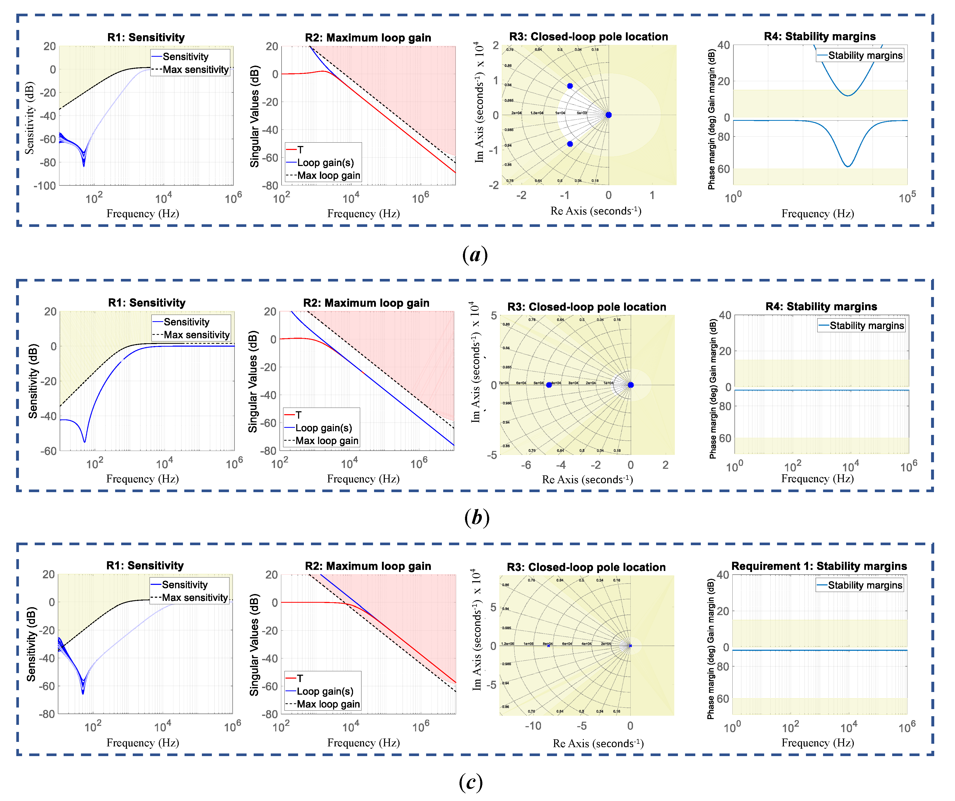
The following design specifications are set up for the current controllers designed by means of the Pole-Placement technique (PP-PI): (i.) a damping factor $\zeta$ equal to $0.707$ and (ii.) a closed-loop bandwidth of 4 kHz. On the other hand, the following goals are established for the current controllers designed based on the structured $H\infty$-norm optimization for both the $H\infty$-PI and $H\infty$-uPI controllers. R1 is a sensitivity function represented by the following transfer function: $S\left(s\right)=1.2s/s+4\times {10}^3$, which guarantees a small gain at low frequencies for good disturbance rejection crossing 0 dB at 4 kHz (the maximum allowed control-loop bandwidth). R2 is the maximum loop gain of $-20$ dB/decade roll-off past 4 kHz, which restricts the maximum control-loop bandwidth. R3 is the specification of the minimum damping and maximum natural frequency for the closed-loop poles, which are $\zeta =0.707$ and ${\omega }_n=12\times {10}^3$ Hz, respectively. R4 is the imposition of a minimum gain margin of 18 dB and a minimum phase margin of 60 degrees. Goals R1, R2, and R3 are defined as soft constraints, while R4 is defined as a hard constraint. Additionally, uncertainties of $30\%$ are considered for L and C and uncertainties of $50\%$ for $R_L$ and $R_0$ to compute the $H\infty$-uPI controllers. A graphical representation of goals R1, R2, and R3 is shown in Figure 5a–c, respectively. In Figure 5, colored areas refer to the forbidden regions that the closed-loop system must avoid.

Regarding the DC-link voltage, the PI controller provides the $i_S^d$ setpoint, when the pole-placement method is used with the following design specifications: i. a damping factor $\zeta$ equal to $0.707$ and ii. a setting time $t_s$ equal to $0.2$ s. The following goals are established for the DC-link voltage PI controller designed, based on the structured $H\infty$-norm optimization for both the $H\infty$-PI and $H\infty$-uPI controllers: R1 is a sensitivity function represented by the following transfer function: $S\left(s\right)=1.2s/s+400$, which guarantees a small gain at low frequencies for good disturbances rejection crossing 0 dB at 400 Hz, the maximum allowed control-loop bandwidth. R2 is the maximum loop gain of $-20$ dB/decade roll-off past $1.6$ kHz, restricting the maximum control-loop bandwidth. R3 is the specification of the minimum damping and maximum natural frequency for the closed-loop poles, which are $\zeta =0.707$ and ${\omega }_n=100$ Hz, respectively. R4 is the imposition of a minimum gain margin of 20 dB and a minimum phase margin of 60 degrees. Goals R1 and R2 are defined as soft constraints, while R3 and R4 are defined as a hard constraints. A graphical representation of goals R1, R2, and R3 is depicted in Figure 6a–c, respectively. In Figure 6, colored areas refer to the forbidden regions that the closed-loop system must avoid.

Table 2. Summary of the PI controller parameters.

Control Loop	PP		$\mathit{H}\mathit{\infty }$-PI				$\mathit{H}\mathit{\infty }$-uPI
	${\mathit{k}}_{\mathit{p}}$	${\mathit{k}}_{\mathit{i}}$	${\mathit{k}}_{\mathit{p}}$	${\mathit{k}}_{\mathit{i}}$	Soft	Hard	${\mathit{k}}_{\mathit{p}}$	${\mathit{k}}_{\mathit{i}}$	Soft	Hard
$i_s^d{u}_d$	−1.7	$-1.55\times {10}^4$	$-0.981$	$-1.16\times {10}^3$	$0.833$	$0.82358$	$-1.23$	$-2.72\times {10}^3$	$0.833$	$0.97621$
$i_s^q{u}_q$	−1.79	$-1.4\times {10}^4$	−4.73	$-4.73\times {10}^{-7}$	$3.91$	$0.69804$	−8.5	$-8.51\times {10}^{-7}$	$7.04$	$0.69804$
$i_s^0{u}_0$	−1.81	$-1.51\times {10}^4$	−1.23	$-2.41\times {10}^3$	$0.833$	$0.88768$	−1.42	$-4.94\times {10}^3$	$0.833$	$0.98983$
$v_{DC}{i}_{s_{REF}}^d$	$0.412$	$29.4$	$0.368$	$5.53$	$2.85$	$0.99984$	$0.234$	$1.73$	$5.8$	$0.99972$

summarizes the PI controller parameters obtained by the pole-placement method and by the $H\infty$ optimization. A value lower than one in the soft and hard columns indicates that the optimization goals were achieved, while a value higher than one indicates that the constraints might be violated. From Table 2, it is remarked that the soft column has few values higher than one, while the hard constraints are fulfilled for all the optimized PI controllers.

Figure 7, Figure 8, Figure 9 and Figure 10 display the optimization constraints and the frequency response of the closed-loop system of every control loop. For instance, from Figure 7, Figure 8, Figure 9 and Figure 10, it is possible to see whether or not the closed-loop specifications are achieved by each of the optimized PI controllers for every control loop. Additionally, it is verified whether the PI controllers tuned via the pole-placement method also meet goals R1, R2, R3, and R4.

Figure 7 presents the results of the $i_s^d$ control loop. Figure 7a shows the closed-loop system frequency response for specifications R1, R2, and R4 and the root location of the closed-loop system verifying specification R3 for the PI controller tuned by using the pole-placement method. From this set of figures, it is possible to observe that specifications R1, R2, and R3 are met, while specification R4 is slightly violated. It is remarked that this R4 refers to the robustness specification, and it was established as a hard constraint for the structured $H\infty$ optimization of the PI controllers. Consequently, it is expected that this PI controller presents a lower robustness than the optimized PI controllers. On the other hand, regarding the optimized PI controllers, from Figure 7b,c, it can be observed that all the specifications are met for $H\infty$-PI and $H\infty$-uPI, respectively.

Figure 8 presents the results of the $i_s^q$ control loop. Figure 8a shows the closed-loop system frequency response for specifications R1, R2, and R4 and the root location of the closed-loop system verifying specification R3 for the PI controller tuned by using the pole-placement method. From this set of figures, it is possible to observe that specifications R1, R2, and R3 are met, while the gain margin part is not achieved for specification R4. This last specification refers to the robustness of the closed-lop system, and it was established as a hard constraint for the structured $H\infty$ optimization; then, it is expected that this PI controller presents lower robustness than the optimized PI controllers for this control loop. Regarding the $H\infty$-PI controller, it is seen from Figure 8b that specification R3 is not fulfilled; however, this specification was given as a soft constraint in the optimization problem. From Figure 8c, it is observed that specification R1 is only violated at low frequencies, while specifications R2 and R3 are not satisfied. It is highlighted from Figure 8b,c that specification R4 is enforced.

Figure 9 presents the results of the $i_s^0$ control loop. It can be seen that all the specifications are achieved; however, the gain margin in specification R4 for the PI controller tuned by means of the pole-placement method is not met. It is expected that the $H\infty$-PI and $H\infty$-uPI controllers are more robust than the pole-placement based PI controller because this restriction R4 was specified as a hard constraint for the $H\infty$ optimization, but it was not met.

Figure 10 presents the results of the $v_{DC}{i}_{s_{REF}^d}$ control loop. Figure 10a shows the closed-loop system frequency response for specifications R1, R2, and R4, as well as the root location of the closed-loop system verifying specification R3 for the PI controller tuned by the pole-placement method. From this set of figures, it is possible to observe that specifications R2 and R3 are met, while specifications R1 and R4 are not satisfied. In particular, it is seen that specification R1 is met at low and high frequencies; however, in an intermediate range, it is violated. Regarding specification R4, neither the phase nor the margin gains are fulfilled, meaning that this PI controller does not meet the robustness criteria. For the $H\infty$-PI and $H\infty$-uPI controllers, it is seen from Figure 8b,c that only specification R1 is not met at low frequencies; nevertheless, this specification was given as a soft constraint in the optimization problem.

As a conclusion from Figure 7, Figure 8, Figure 9 and Figure 10, all hard constraints are enforced, and the pole-placement PI controllers meet all specifications of the optimal controllers; however, the robustness constraint given by specification R4 is not met. This means that in the case of not having high parametric uncertainties, all obtained PI controllers should perform very similarly. To validate the above statement, simulations in PSIM comparing the closed-loops dynamical performance were carried out. Accordingly, starting from the nominal load, that is for $R=18.58$ $\Omega$ and $L=44$ mH, four step changes represented as load variations were applied to the TLSC SAPF as follows: i. At $t=0.7$ s, an unbalanced system condition was set up, a total equivalent inductive-resistive load with $L=1$ mH and $R_a=17$ $\Omega$, $R_b=18$ $\Omega$, and $R_c=38$ $\Omega$ is connected in shunt form to phases a, b, and c, respectively, to the nominal load. Next, ii. at $t=1.4$ s, a harmonic and inductive-resistive load with $L=1$ mH and $R=17$ $\Omega$ was added in parallel to the previous equivalent unbalanced load. This configuration represents a harmonic-unbalanced load, and it is the worst condition considered in this study. iii. At $t=1.7$ s, both the nominal and the unbalanced loads are removed, leaving only the harmonic and inductive-resistive load with $L=1$ mH and $R=17$ $\Omega$. Finally, iv. at $t=2.2$ s, the load is disconnected, the TLSC SAPF being the only remaining load to the main grid. Thus, from $t=2.2$ to $t=2.4$, it is possible to obverse how much power the converter is demanding from the grid and whether it is active or reactive power. The total simulation time is $t=2.4$ s.

Figure 11 shows the comparison between all the designed PI controllers. From Figure 11a–c, it is possible to appreciate that all the PI current controllers perform quite similarly, satisfactorily tracking the current references even when these are sinusoidal signals. Additionally, it is observed from the simulation results that the zero current component is different from zero only when the unbalanced load is connected to the grid and the $dq$ current components track sinusoidal references. Furthermore, it is observed that the q current component predominates in the time interval when only the harmonic load is considered, meaning that most of the harmonics are related to load inefficiencies. Regarding the DC-link voltage loop simulations reported in Figure 11d, it is appreciated that the designed PI controllers can regulate the voltage to 600 V, rejecting all the disturbances due to the load variations. It is also observed that a small oscillation appears during the time interval in which the unbalanced condition of the load is simulated. However, this oscillation is considerably small and does not affect the control loop performance. Finally, it is highlighted that the maximum voltage overshoot is around $3\%$, showing the control structure’s capabilities to preserve the system stability.

The simulation results displayed in Figure 11 validate that all the designed PI controllers satisfactorily achieve the control objectives. However, it is not possible to quantitatively establish which one performs better.

Table 3. Summary of the PI controller dynamical performance indices.

		Performance Indices
Control Loop	Controller Type	IAE	ITAE	IAU	${\mathit{M}}_{\mathit{s}}$
$i_s^d{u}_d$	PP-PI	$0.2968$	$0.5187$	$0.3630$	$2.20$
	$H\infty$-PI	$0.0756$	$0.1137$	$0.1755$	$0.66$
	$H\infty$-uPI	$0.0710$	$0.1071$	$0.1746$	$0.98$
$i_s^q{u}_q$	PP-PI	$0.0532$	$0.0792$	$0.2845$	$2.01$
	$H\infty$-PI	$0.0459$	$0.0714$	$0.2127$	$0.00$
	$H\infty$-uPI	$0.0456$	$0.0674$	$0.3786$	$0.00$
$i_s^0{u}_0$	PP-PI	$0.1095$	$0.1665$	$0.2862$	$1.99$
	$H\infty$-PI	$0.1051$	$0.1579$	$0.1358$	$0.85$
	$H\infty$-uPI	$0.1035$	$0.1561$	$0.1616$	$1.25$
$v_{DC}{i}_{s_{REF}}^d$	PP-PI	$2.5332$	$4.1969$	$1.8025$	$2.66$
	$H\infty$-PI	$2.3525$	$3.7953$	$1.8095$	$0.70$
	$H\infty$-uPI	$3.1735$	$5.1753$	$1.8730$	$0.72$

summarizes the PI controller dynamical performance indices $IAE$ and $ITAE$, the control action effort index $IUA$, and the maximum sensitivity $M_s$. From Table 3, it is possible to conclude that for the current control loops, in general, $H\infty$-uPI controllers perform better than $H\infty$-PI and PP-PI controllers; whereas, $H\infty$-PI controllers turned out to be more robust for the performed simulations. However, it is expected that $H\infty$-uPI controllers perform better in highly uncertainty situations. Regarding the DC-link voltage control loop, the $H\infty$-PI controller turned out to perform better than the $H\infty$-uPI and PP-PI controllers. However, again, the $H\infty$-uPI controller is expected to perform better in highly uncertain scenarios. It is worth mentioning that despite the differences in the performance indices, all the designed PI controllers present a good dynamical performance, tracking complex current references and preserving the global stability of the control structure despite the applied load variations and their nonlinearities.

4.3. TLSC SAPF Compensation Performance

From the results reported in Figure 11, it is clear that each of the designed PI controllers is suitable to perform its functions. The question now is whether the whole control structure achieves the control objective; that is, the TLSC SAPF provides the load of all the currents associated with inefficient powers while regulating the DC-link voltage and minimizing the neutral current. Accordingly, other simulations are performed in PSIM to evaluate to what extent this control objective is achieved. These simulations are carried out only considering the $H\infty$-uPI controllers and adopting the same simulation setup as in the PI controllers’ performance evaluation. From Figure 11, it is possible to validate that the DC-link voltage is regulated at 600 V independently of the load variations. On the other hand, Figure 12 shows the $dq0$ components of the currents and the neutral current on the grid, load, and converter sides. Figure 12a shows the d current component. There, it is observed that the sum of $i_{grid}^d$ and $i_S^d$ results in $i_{Load}^d$, where $i_S^d$ is composed of the oscillatory part of $i_{Load}^d$ and a small DC quantity related to the demanded current by the TLSC SAPF to supply its internal losses and maintain the DC-link voltage level. This means that $i_{grid}^d$ is mainly composed of efficient currents. Figure 12b displays the q current component. From this Figure, it is observed that $i_{grid}^q$ remains close to zero during the whole simulation time, meaning that no inefficient currents related to the demanded reactive power are supplied by the grid. Indeed, it is observed that $i_L^q$ and $i_S^q$ are opposite, meaning that $i_S^q$ corresponds to the q current component demanded by the load. Figure 12c presents the results of the zero current component. This figure shows that $i_{Load}^0$ is different from zero within the time interval $0.7$ s to $1.7$ s, meaning that an unbalanced load condition in fact causes the appearance of the neutral current. However, $i_{grid}^0$ remains close to zero during the whole simulated time, which indicates that the $i_S^0{u}_0$ control loop effectively compensates the inefficient currents related to the load unbalances. The above statement is validated by Figure 12d, where it is appreciated that the neutral current returning to the grid is close to zero during the whole simulated time, while the neutral current by the converter and the load cancel out each other.

Figure 13 shows the currents per phase in the $abc$ reference frame for $i_{grid}^{abc}$, $i_{Load}^{abc}$, and $i_S^{abc}$, comparing them with respect to the voltage at the common coupling point (PCC). The aim is to verify whether currents and voltage are in or out of phase. Figure 13a compares the $abc$ current components on the grid, load, and converter sides from left to right, respectively. From the left-hand figure, it is possible to appreciate that the currents on the grid side remain balanced for the unbalanced and harmonic load conditions. The figure in the middle shows the waveform of the current demanded by the load. It is observed how, in the time interval $0.7$ s to $1.2$ s, phase c demands a lower current than phases a and b, while, in the time interval $1.8$ s to $2.2$ s, the demanded current has harmonic distortion. The right-hand side of Figure displays the currents related to the converter side. It is observed that the waveform of the currents at this side seems to correspond to the inefficient currents demanded by the load. For instance, by the zoom at $t=2$ s, it is seen that the current waveform is very distorted, which can be associated with the harmonics caused by the harmonic load. Figure 13b–d displays the currents on each side of the system and compares them to the voltage at the PCC. From this set of figures, it can be seen that the only currents remaining in phase with the voltage at the PCC are those at the grid side. In contrast, the currents on the load and converter sides are all out of phase for the time intervals in which the load is unbalanced. Additionally, for the time interval in which the harmonic load condition is considered, it is possible to appreciate how the currents on the converter side become distorted.

In conclusion, from Figure 11, Figure 12 and Figure 13, it is possible to appreciate that the TLSC SAPF achieves the control objective, leaving to the grid the task of only supplying the considered efficient currents to the load. Moreover, the neutral current returning to the grid is minimized, and the DC-link voltage level is regulated, at the same time only with the proposed control structure based on simple feedback control loops and composed of standard PI controllers.

5. Conclusions

This paper introduced a dynamical-based model approach for controlling TLSC SAPFs; the reactive, unbalanced, and harmonic compensation, as well as the regulation of the DC-link bus were successfully achieved. The $dq0$ model for TLSC SAPFs, which includes power losses, was deduced; both large- and small-signal models were presented to have ready-to-use models for design and control purposes. Furthermore, transfer functions and steady-state analysis were included in the procedure. It is remarked that the objective control was fulfilled by using a simple feedback control structure composed of standard PI controllers.

Controllability was evaluated through a set-theoretic approach, obtaining the reversible and reachable sets’ hypervolumes and concluding that TLSC SAPF is locally controllable around its operating point. For the particular case evaluated, the controllability index was $67.72\%$, which indicates that there is a portion of the space-state reachable with the admissible control actions; the other uncontrollable portion that corresponds to the region when $t>50$ ms is considered a safe region since the switching time is $0.05$ ms.

Robust controllers based on PP-PI, $H\infty$, and $H\infty$-uPI controllers were satisfactorily implemented. The $H\infty$ and $H\infty$-uPI controller parameters were obtained through an optimization process. A detailed comparison among controllers was performed though the evaluation of $IAE$, $ITAE$, $IUA$, and $M_s$. The tests showed that all designed controllers performed very similarly and were capable of rejecting several types of disturbances while preserving the system stability; however, it was found that the $H\infty$-uPI controller performed better under highly uncertainty scenarios.

References

- Tofoli, F.; Sanhueza, S.; de Oliveira, A. On the study of losses in cables and transformers in nonsinusoidal conditions. IEEE Trans. Power Deliv. 2006, 21, 971–978. [Google Scholar] [CrossRef]
- Artemenko, M.; Batrak, L.; Polishchuk, S.; Mykhalskyi, V.; Shapoval, I. Minimization of cable losses in three-phase four-wire systems by means of instantaneous compensation with shunt active filters. In Proceedings of the 2013 IEEE XXXIII International Scientific Conference, Electronics and Nanotechnology (ELNANO), Kiev, Ukraine, 16–19 April 2013; pp. 359–362. [Google Scholar] [CrossRef]
- Said, D.; Nor, K. Effects of harmonics on distribution transformers. In Proceedings of the 2008 AUPEC’08 Australasian Universities, Power Engineering Conference, Sydney, Australia, 14–17 December 2008; pp. 1–5. [Google Scholar]
- Liu, R.; Mi, C.; Gao, D. Modeling of Eddy-Current Loss of Electrical Machines and Transformers Operated by Pulsewidth-Modulated Inverters. IEEE Trans. Magn. 2008, 44, 2021–2028. [Google Scholar] [CrossRef]
- Thapar, A.; Saha, T.; Dong, Z.Y. Investigation of power quality categorisation and simulating it’s impact on sensitive electronic equipment. In Proceedings of the 2004 IEEE Power Engineering Society General Meeting, San Francisco, CA, USA, 12–16 June 2004; Volume 1, pp. 528–533. [Google Scholar] [CrossRef] [Green Version]
- Pindado, R.; Rodríguez, P.; Pou, J.; Candela, I. Controller for Three-Phase Four-Wire Shunt Active Power Filter by DC-Bus Energy Regulation. Renew. Energy Power Qual. J. 2004, 1, 371–378. [Google Scholar] [CrossRef]
- Rafi, F.H.M.; Hossain, M.; Rahman, M.S.; Taghizadeh, S. An overview of unbalance compensation techniques using power electronic converters for active distribution systems with renewable generation. Renew. Sustain. Energy Rev. 2020, 125, 109812. [Google Scholar] [CrossRef]
- Khadkikar, V.; Chandra, A.; Singh, B. Digital signal processor implementation and performance evaluation of split capacitor, four-leg and three H-bridge-based three-phase four-wire shunt active filters. IET Power Electron. 2011, 4, 463–470. [Google Scholar] [CrossRef]
- Cao, W.; Liu, K.; Wu, M.; Xu, S.; Zhao, J. An Improved Current Control Strategy Based on Particle Swarm Optimization and Steady-State Error Correction for SAPF. IEEE Trans. Ind. Appl. 2019, 55, 4268–4274. [Google Scholar] [CrossRef]
- Pandove, G.; Singh, M. Robust Repetitive Control Design for a Three-Phase Four Wire Shunt Active Power Filter. IEEE Trans. Ind. Inform. 2019, 15, 2810–2818. [Google Scholar] [CrossRef]
- Zhang, Y.; Dai, K.; Chen, X.; Kang, Y.; Dai, Z. Stability Analysis of SAPF by Viewing DFT as Cluster of BPF for Selective Harmonic Suppression and Resonance Damping. IEEE Trans. Ind. Appl. 2019, 55, 1598–1607. [Google Scholar] [CrossRef]
- Mu, X.; Wang, J.; Wu, W.; Blaabjerg, F. A Modified Multifrequency Passivity-Based Control for Shunt Active Power Filter with Model-Parameter-Adaptive Capability. IEEE Trans. Ind. Electron. 2018, 65, 760–769. [Google Scholar] [CrossRef]
- Xu, C.; Dai, K.; Chen, X.; Peng, L.; Zhang, Y.; Dai, Z. Parallel Resonance Detection and Selective Compensation Control for SAPF with Square-Wave Current Active Injection. IEEE Trans. Ind. Electron. 2017, 64, 8066–8078. [Google Scholar] [CrossRef]
- Muñoz-Galeano, N.; Orts-Grau, S.; Seguí-Chilet, S.; Gimeno-Sales, F.J.; López-Lezama, J.M. Deterministic Algorithm for Selective Shunt Active Power Compensators According to IEEE Std. 1459. Energies 2017, 10, 1791. [Google Scholar] [CrossRef] [Green Version]
- Bacha, S.; Munteanu, I.; Bratcu, A. General Control Principles of Power Electronic Converters. In Power Electronic Converters Modeling and Control; Advanced Textbooks in Control and Signal Processing; Springer: London, UK, 2014; pp. 179–186. [Google Scholar] [CrossRef]
- Hägglund, T. The one-third rule for PI controller tuning. Comput. Chem. Eng. 2019, 127, 25–30. [Google Scholar] [CrossRef]
- Apkarian, P.; Noll, D. Optimization-Based Control Design Techniques and Tools. In Encyclopedia of Systems and Control; Springer: London, UK, 2015; pp. 1–12. [Google Scholar] [CrossRef] [Green Version]
- Apkarian, P.; Noll, D. The H∞ Control Problem is Solved. Aerosp. Lab 2017, 1–11. [Google Scholar] [CrossRef]
- Apkarian, P.; Dao, M.N.; Noll, D. Parametric Robust Structured Control Design. IEEE Trans. Autom. Control 2015, 60, 1857–1869. [Google Scholar] [CrossRef] [Green Version]
- Panigrahi, R.; Subudhi, B. Performance Enhancement of Shunt Active Power Filter Using a Kalman Filter-Based H-∞ Control Strategy. IEEE Trans. Power Electron. 2016, 32, 2622–2630. [Google Scholar] [CrossRef]
- Huang, L.; Xin, H.; Dörfler, F. H-∞-Control of Grid-Connected Converters: Design, Objectives and Decentralized Stability Certificates. IEEE Trans. Smart Grid 2020. [Google Scholar] [CrossRef]
- Bouzid, A.M.; Sicard, P.; Cheriti, A.; Bouhamida, M.; Benghanem, M. Structured H-∞ design method of PI controller for grid feeding connected voltage source inverter. In Proceedings of the 2015 IEEE 3rd International Conference on Control, Engineering & Information Technology (CEIT), Tlemcen, Algeria, 25–27 May 2015; pp. 1–6. [Google Scholar]
- Li, X.; Zhang, Z. Study on the output controllability of BUCK-BOOST Converter. In Proceedings of the 2017 IEEE International Conference on Mechatronics and Automation (ICMA), Takamatsu, Japan, 6–9 August 2017; pp. 107–112. [Google Scholar]
- Kalman, R. On the general theory of control systems. IRE Trans. Autom. Control 1959, 4, 110. [Google Scholar] [CrossRef]
- Bhattacharyya, D.; Pati, K.C. Controllability analysis for switched linear system model of DC-DC flyback converter using controllability transition approach. Int. J. Control 2020, 1–9. [Google Scholar] [CrossRef]
- Osorio, J.C.C. Una Aproximación al Diseño y Control Total de Planta Usando Controlabilidad de Estado. Doctorado en Ingeniería—Sistemas Energéticos Línea de Investigación: Diseño y Control de Procesos Químicos. Ph.D. Thesis, Universidad Nacional de Colombia Sede Medellín, Antioquia, Colombia, 2013. [Google Scholar]
- García, P. Efecto de las Condiciones Iniciales Sobre la Controlabilidad de Estado en Procesos por Lotes. Magister en Ingeniería Química. Master’s Thesis, Universidad Nacional de Colombia, Sede Medellín, Facultad de Minas, Antioquia, Colombia, 2012. [Google Scholar]
- Alzate, A.; Gómez, L.; Alvarez, H. Diseño Simultáneo de Procesos y su control usando Teoría de Conjuntos. Prospect 2015, 13, 12–23. [Google Scholar] [CrossRef] [Green Version]
- Calderón, C.; Gómez, L.; Alvarez, H. Nonlinear state space controllability: Set theory vs differential geometry. In Proceedings of the Congreso Latinoamericano de Control Automático, Lima, Peru, 23–26 October 2012. [Google Scholar]
- Gómez, L.; Botero, H.; Alvarez, H.; di Sciascio, F. Análisis de la Controlabilidad de Estado de Sistemas Irreversibles Mediante Teoría de Conjuntos. Rev. Iberoam. Automática Informática Industrial {RIAI} 2015, 12, 145–153. [Google Scholar] [CrossRef] [Green Version]
- Escobar, G.; Valdez, A.; Torres-Olguin, R.; Martinez-Montejano, M. A Model-Based Controller for a Three-Phase Four-Wire Shunt Active Filter with Compensation of the Neutral Line Current. IEEE Trans. Power Electron. 2007, 22, 2261–2270. [Google Scholar] [CrossRef]
- Orts-Grau, S.; Gimeno-Sales, F.; Segui-Chilet, S.; Abellan-Garcia, A.; Alcaniz, M.; Masot-Peris, R. Selective Shunt Active Power Compensator Applied in Four-Wire Electrical Systems Based on IEEE Std. 1459. IEEE Trans. Power Deliv. 2008, 23, 2563–2574. [Google Scholar] [CrossRef]
- Orts-Grau, S.; Gimeno-Sales, F.; Abellan-Garcia, A.; Segui-Chilet, S.; Alfonso-Gil, J. Improved Shunt Active Power Compensator for IEEE Standard 1459 Compliance. IEEE Trans. Power Deliv. 2010, 25, 2692–2701. [Google Scholar] [CrossRef] [Green Version]
- Choi, W.H.; Lam, C.S.; Wong, M.C.; Han, Y.D. Analysis of DC-Link Voltage Controls in Three-Phase Four-Wire Hybrid Active Power Filters. IEEE Trans. Power Electron. 2013, 28, 2180–2191. [Google Scholar] [CrossRef]
- Sun, Z.; Zhang, Z.; Tsao, T.C. Trajectory tracking and disturbance rejection for linear time-varying systems: Input/output representation. Syst. Control Lett. 2009, 58, 452–460. [Google Scholar] [CrossRef]
- Montero, M.; Cadaval, E.; Gonzalez, F. Comparison of Control Strategies for Shunt Active Power Filters in Three-Phase Four-Wire Systems. IEEE Trans. Power Electron. 2007, 22, 229–236. [Google Scholar] [CrossRef]
- Reginatto, R.; Ramos, R. On electrical power evaluation in dq coordinates under sinusoidal unbalanced conditions. IET Gener. Transm. Distrib. 2014, 8, 976–982. [Google Scholar] [CrossRef] [Green Version]
- Po-Ngam, S. The simplified control of three-phase four-leg shunt active power filter for harmonics mitigation, load balancing and reactive power compensation. In Proceedings of the 2014 11th International Conference on Electrical Engineering/Electronics, Computer, Telecommunications and Information Technology (ECTI-CON), Nakhon Ratchasima, Thailand, 14–17 May 2014; pp. 1–6. [Google Scholar]
- Orts, S.; Gimeno-Sales, F.; Abellan, A.; Segui-Chilet, S.; Alcaniz, M.; Masot, R. Achieving Maximum Efficiency in Three-Phase Systems with a Shunt Active Power Compensator Based on IEEE Std. 1459. IEEE Trans. Power Deliv. 2008, 23, 812–822. [Google Scholar] [CrossRef]
- Tang, Y.; Loh, P.C.; Wang, P.; Choo, F.H.; Gao, F.; Blaabjerg, F. Generalized Design of High Performance Shunt Active Power Filter with Output LCL Filter. IEEE Trans. Ind. Electron. 2012, 59, 1443–1452. [Google Scholar] [CrossRef]
- Apkarian, P.; Noll, D. Nonsmooth H-∞ Synthesis. IEEE Trans. Autom. Control 2006, 51, 71–86. [Google Scholar] [CrossRef] [Green Version]
- Gómez, L. Una Aproximación al Control de los Procesos por Lotes. Ph.D. Thesis, Facultad de Ingeniería, Universidad Nacional de San Juan, San Juan, Argentina, 2009. [Google Scholar]
- Alzate, A. Metodología Para el Diseño Simultáneo de Equipo y su Sistema de Control Robusto. Master’s Thesis, Universidad Nacional de Colombia, Medellín, Colombia, 2013. [Google Scholar]
- Zouidi, A.; Fnaiech, F.; Al-Haddad, K. Voltage source Inverter Based three-phase shunt active Power Filter: Topology, Modeling and Control Strategies. In Proceedings of the 2006 IEEE International Symposium on Industrial Electronics, Montreal, QC, Canada, 9–13 July 2006; Volume 2, pp. 785–790. [Google Scholar] [CrossRef]
- IEEE Standards 519-2014. IEEE Recommended Practice and Requirements for Harmonic Control in Electric Power Systems; IEEE: Piscataway, NJ, USA, 2014. [Google Scholar]
- Louganski, K.; Lai, J.S. Current Phase Lead Compensation in Single-Phase PFC Boost Converters with a Reduced Switching Frequency to Line Frequency Ratio. IEEE Trans. Power Electron. 2007, 22, 113–119. [Google Scholar] [CrossRef]
- Vilanova, R.; Alfaro, V.M. Control {PID} robusto: Una visión panorámica. Rev. Iberoam. Automática Informática Ind. {RIAI} 2011, 8, 141–158. [Google Scholar] [CrossRef] [Green Version]
- Zeng, F.P.; Tan, G.H.; Wang, J.Z.; Ji, Y.C. Novel single-phase five-level voltage-source inverter for the shunt active power filter. IET Power Electron. 2010, 3, 480–489. [Google Scholar] [CrossRef]
- Danyali, S.; Hosseini, S.; Gharehpetian, G. New Extendable Single-Stage Multi-input DC-DC/AC Boost Converter. IEEE Trans. Power Electron. 2014, 29, 775–788. [Google Scholar] [CrossRef]
- Li, X.; Zhang, B.; Qiu, D.; Wang, D. New PWM strategy for nine-switch inverters with minimum number of semiconductor switching. In Proceedings of the 2014 International Electronics and Application Conference and Exposition (PEAC), Shanghai, China, 5–8 November 2014; pp. 406–410. [Google Scholar] [CrossRef]
- Li, X.; Zhang, B.; Qiu, D. Three-mode pulse-width modulation of a three-phase four-wire inverter. IET Power Electron. 2015, 8, 1483–1489. [Google Scholar] [CrossRef]
- Urrea-Quintero, J.H.; Hernández, H.; Ochoa, S. Towards a controllability analysis of multiscale systems: Application of the set-theoretic approach to a semi-batch emulsion polymerization process. Comput. Chem. Eng. 2020, 106833. [Google Scholar] [CrossRef]
- Sontag, E. Mathematical Control Theory; Texts in Applied Mathematics; Springer: New York, NY, USA, 1998. [Google Scholar]
- Tempo, R.; Calafiore, G.; Dabbene, F. Randomized Algorithms for Analysis and Control of Uncertain Systems: With Applications; Springer: London, UK, 2013. [Google Scholar]
Figure 1.
Three-Leg Split-Capacitor (TLSC) SAPF circuit representation.
Figure 2.
TLSC SAPF control structure.
Figure 3.
The TLSC SAPF equivalent simplified representation assuming a perfect control of .
Figure 4.
Reachable set from at ms and controllable set to in ms for the TLSC SAPF.
Figure 5.
Closed-loop specifications for the structured PI structured controllers: (a) R1 sensitivity function, (b) R2 maximum loop gain, and (c) R3 minimum damping and maximum natural frequency for the closed-loop poles.
Figure 6.
Closed-loop specifications for the structured DC-link PI structured controller: (a) R1 sensitivity function, (b) R2 maximum loop gain, and (c) R3 minimum damping and maximum natural frequency for the closed-loop poles.
Figure 7.
Closed-loop specifications’ verification for the loop: (a) Pole-Placement (PP)-PI, (b) -PI, and (c) -uPI.
Figure 8.
Closed-loop specifications’ verification for the loop: (a) PP-PI, (b) -PI, and (c) -uPI.
Figure 9.
Figure 10.
Figure 11.
PI controllers’ dynamical performance comparison: (a) , (b) , (c) , and (d) .
Figure 12.
Figure 13.
PI controllers dynamical performance comparison: (a) , (b) , (c) , and (d) .