Abstract
In this paper, we applied a system identification algorithm and an adaptive controller to a simple kite system model to simulate crosswind flight maneuvers for airborne wind energy harvesting. The purpose of the system identification algorithm was to handle uncertainties related to a fluctuating wind speed and shape deformations of the tethered membrane wing. Using a pole placement controller, we determined the required locations of the closed-loop poles and enforced them by adapting the control gains in real time. We compared the path-following performance of the proposed approach with a classical proportional-integral-derivative (PID) controller using the same system model. The capability of the system identification algorithm to recognize sudden changes in the dynamic model or the wind conditions, and the ability of the controller to stabilize the system in the presence of such changes were confirmed. Furthermore, the system identification algorithm was used to determine the parameters of a kite with variable-length tether on the basis of data that were recorded during a physical flight test of a 20 kW kite power system. The system identification algorithm was executed in real time, and significant changes were observed in the parameters of the dynamic model, which strongly affect the resulting response.
1. Introduction
Airborne wind energy (AWE) is an emerging renewable energy technology that uses flying devices that are tethered to the ground [1,2,3]. Compared to horizontal axis wind turbines (HAWTs), AWE systems have a number of distinct advantages in terms of costs, maintenance, operating altitude, and capacity factor. However, as wind turbines have matured over decades of continuous research and development, AWE technologies, which are at a comparatively early stage of development, are still considered to be less reliable. For a HAWT, almost of the power is generated by the tip of the rotor blades, while the rest of the rotor functions mainly as a support structure for the crosswind motion of the blades [1,2,4]. The rated power of the generator typically determines the installation. For the same rated power, an AWE system generally gives a higher annual yield than a HAWT because it can operate at a higher capacity factor. This higher capacity factor is a result of the more persistent and more steady wind at higher altitudes. However, an AWE system also needs more space than a HAWT, which increases the costs of an installation. These land surface costs are still quite unknown and responsible for the large differences in expected costs [5,6].
There are several different concepts and configurations of AWE systems [2,7]. A comparatively simple one is the pumping kite power system illustrated in Figure 1. The kite consists of a flexible membrane wing that is steered by a suspended kite control unit (KCU) and tethered to a drum on the ground that is coupled to a generator. During the reel out of the tether, the kite is operated in crosswind figure-of-eight maneuvers, as shown in Figure 2, to maximize the pulling force and thus generated energy when pulling the tether from the drum. When reaching the maximal tether length, the kite is depowered and retracted, using the generator as a motor and consuming a fraction of the formerly generated energy. The change of the flight patterns between reel-out and reel-in phases results in a net energy per pumping cycle [5,8]. The main objective of the control algorithm is to ensure the robust and safe flight operation of the kite.
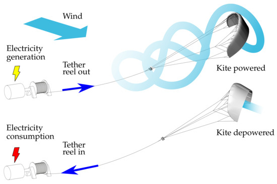
Figure 1.
Working principle of the pumping kite power system of Delft University of Technology [5].
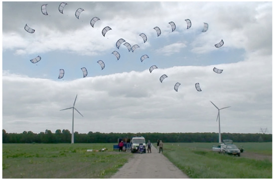
Figure 2.
Composite photo of a crosswind figure-of-eight maneuver ( s) of a tube kite with 25 m wing surface area [9].
Several mathematical models have been developed to describe the dynamic behavior of a kite system [1,3,10,11]. Obvious shortcomings of these models are the numerous idealizations that limit the achievable prediction quality for a flight trajectory in a real wind environment, which is characterized by local changes in wind speed and direction occurring within seconds [12,13]. Another modeling challenge is the aeroelastic response of the membrane wing because substantial deformations also majorly affect the aerodynamic properties of the kite system [14,15,16].
Generally, in most control applications, the mathematical model can be based on either (1) a system that has a fixed operating point and control parameters that are fixed due to the stability in the model, or (2) a system that has a variable operating point, requiring that it is robust enough to sustain the variation. The dynamic model representing a kite system is of the latter type, since the system characteristics are time-varying due to the natural fluctuations of the wind environment. This has to be considered in the design of the control algorithm for the kite system.
In recent years, research on kite control has considerably intensified [17,18,19,20]. The developed models are typically based on state-space representations of a real AWE system, describing the nonlinear dynamics of 4 up to 15 states. In [21], the optimal flight path is determined ahead of time using nonlinear model predictive control (NMPC). However, this control method is computationally expensive and with additional expenses for solving the nonlinear optimization problem [19,20]. For this reason, we considered the method unsuitable for real-time control of AWE systems.
Several open-source software tools for AWE systems have been developed over the past few years [11,22,23]. These tools are suitable for computational simulation of flight maneuvers, virtual testing of flight-control algorithms, and optimizing flight paths in real time. One particular aspect of modeling is the flexible tether that is deployed from the ground station and sweeping through the wind field, while being exposed to a distributed aerodynamic load and gravity [24]. A common assumption is that of a perfectly tensioned straight tether. While generally valid during the traction phase, this assumption is not acceptable during the retraction, landing, and take-off phases. Because of the low tension, tether sag has to be taken into account in the modeling [8,25].
The control approach proposed in [26] is interesting because it does not require any information about the kite or the wind field. Although the approach allows for the high-precision tracking of figure-of-eight maneuvers, this is only feasible for a short tether of constant length. The approach is not suitable, however, for a long or variable-length tether [12]. The research challenges addressed in this work can be summarized as follows:
- The kite is based on a flexible membrane wing, and its shape depends on the aerodynamic force distribution during flight, the structural design, and the line suspension system;
- the relative flow velocity experienced by wing and tether varies along the flight path, and there is yet no accurate way to assess this in real time; and
- an accurate estimation of the wind field is necessary to determine the aerodynamic force distribution on tether and wing surface [4,5].
As a result of this physical complexity, there is a crucial need for robust control to stabilize the kite in real time. The above challenges were addressed as follows:
- We propose an algorithm that estimates the parameters of the kite’s dynamic model in real time using system identification (SI) [27,28,29,30]. The employed SI algorithm is a noniterative technique based on Plackett’s algorithm due to its ability to calculate the parameters of the system (dynamic model) with high accuracy without singularity.
- We further propose an adaptive controller to improve the robustness of the system and stabilize the kite in different wind conditions. Moreover, SI is considered as a part of the adaptive control strategy, and the estimated parameters are used to obtain the control gains [30], which means that these gains are updated in real time on the basis of changes in the dynamic model [28].
- We present a comparison between adaptive and classical controllers to highlight the robustness of the controller and the ability of adaptive control to stabilize the kite for different wind conditions without any change in the SI and adaptive control algorithms.
- We applied the SI algorithm to experimental data of the 20 kW kite power system of Delft University of Technology [5]. The algorithm was used to estimate the parameters of the system in different operating phases, such as tether reel out and reel in, for two consecutive pumping cycles while experiencing changes in wind speed and tether length.
The remainder of this paper is divided as follows. Section 2 outlines the components of the mathematical model, and discusses it briefly on the basis of the concepts and implementations described in [12,28]. The mathematical model includes a simplified kite system model, designed as a single-input single-output (SISO) model relating the relative steering input (input) to the course angle (output) of the kite, a flight path planner (FPP), and a flight path controller (FPC). In Section 3 the derivation and implementation of the SI algorithm is discussed in detail. Subsequently, Section 4 presents the adaptive controller based on the estimated parameters from the SI algorithm that is used to stabilize the kite in real time. In Section 5, simulation results are presented for the classical controller described in [12,13,28], and for the combination of adaptive controller and SI algorithm, and compared for two different flight conditions. Finally, Section 6 summarizes the experimental results using measurement data acquired during a physical flight test; then, these results are analyzed using the SI algorithm derived in Section 3. Section 7 concludes this article.
2. Mathematical Model
The approach presented in this paper was derived for the 20 kW kite power system of Delft University of Technology, as illustrated in Figure 1 and Figure 2. The mathematical model was previously formulated and demonstrated in [12,28]. The flight path planning (FPP) and flight path control (FPC) approaches were both designed on the basis of this model. The presented simulation results were obtained by a Simulink/MATLAB® implementation.
2.1. Simplified Kite System Model
To describe the flight motion of the kite power system, we introduce the wind reference frame (), the kite reference frame (), and the small earth reference frame (), as illustrated in Figure 3.
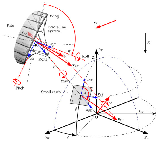
Figure 3.
Reference frames to describe kite tethered flight, heading angle , and course angle .
The wind reference frame is attached to the tether exit point at the ground station and rotates with the wind around its -axis, such that its -axis is always aligned with the instantaneous wind direction. It is assumed that this rotation is slow compared to the flight dynamics of the kite, such that any induced forces can be neglected. The body-fixed kite reference frame is attached to the center of mass of the kite, and accounts for wing, bridle line system, and the suspended kite control unit (KCU). To obtain the co-ordinates of the kite in the small earth reference frame [31], its position is radially projected onto the unit sphere around the tether exit point . On the unit sphere, we define a local tangential plane . The position of the kite in the small earth reference frame can be described by the azimuth angle and the elevation angle , which represent the latitude and longitude of the position, respectively. The velocity of the kite can be decomposed into a radial component and a tangential component , which can be derived from the kite position as
The course angle is defined as the angle between and the upwards direction, represented by the local -axis [12,13]. The heading angle describes the orientation of the kite in the tangential plane, and is defined as the angle between the -axis and the upwards direction. The course angle generally follows the heading angle with a varying offset due to gravity. The angular velocity of the kite with respect to the origin is kinematically coupled to the tangential velocity of the kite
where is the vector pointing from origin to kite . The relative flow velocity at the kite is computed from the wind and kite velocity vectors as
To simplify the FPP and FPC implementations, we introduce the following assumptions that are valid for the traction phase when the tether is generally fully tensioned:
- The tether is straight, and the tether length is identical to the radial position r of the kite .
- The wing is attached to the tether with a bridle line system that constrains the roll and pitch of the wing. Only the heading angle remains as a degree of freedom to control the course of the kite.
- The difference between heading and course angles can be neglected. Both angles and their time derivatives are assumed to be identical in this study.
By decomposing the kite velocity into radial and tangential components, we essentially decouple the flight control of the kite from the winch control. The kite is steered by actuation of the rear bridle line system, which is quantified by the relative steering that can vary between −1 and 1. Additional inputs of the kite model are the magnitude of the apparent wind speed , the initial elevation angle , the angular speed , and the initial values for the course angle and the azimuth angle . The outputs of this model are the course angle , its time derivative , and the position of the kite in terms of elevation angle and azimuth angle .
To calculate the angular speed of the kite, we use the simplified kite system model that was derived in [12]. In this model, which was also used in [28], it is assumed that the angular speed is a function of only the elevation angle . The angular speed is zero at the maximal value and increases linearly with decreasing elevation angle, until it reaches a specific value at . This behavior is described by the following correlation:
Flight tests of the TU Delft Hydra kite [5,8] showed that the maximal elevation angle was reached when the kite was statically positioned at a tether length of 300 m at an approximate ground wind speed of 6 m/s. We further assume that the value is a linear function of the apparent wind speed , which can be expressed as
where denotes the angular speed that is reached at a specific apparent wind speed . On the basis of the flight test data, we determined an angular speed deg/s for an elevation angle and an apparent wind velocity m/s. Combining Equations (6) and (7), we can calculate the angular speed of the kite as a function of the elevation angle and the apparent wind velocity . Multiplying the angular speed of the kite with the radial co-ordinate r, we can calculate the tangential speed , as described by Equation (4).
We determine the course angle of the kite by integrating the turn rate law, which is an empirical correlation between the rate of change of the heading angle (identical to the rate of change of the course angle), the apparent wind speed , and the relative steering action [12,26,28]:
The second term in Equation (8) quantifies the effect of gravity on the turn rate. In the next step, we combine Equations (2) and (4) to eliminate , and calculate the time derivatives of the azimuth and elevation angles from the angular speed . These derivatives are integrated to determine the angular position of the kite.
To summarize, the simplified kite model describes a single-input single-output (SISO) system. The model is characterized by two position and two velocity state variables, (, ) and (, ), respectively, three steering parameters (, , ), and one relative steering action .
2.2. Flight Path Planner (FPP)
The purpose of the FPP is to design a suitable flight trajectory for a pumping cycle. The path is constructed in the - space as a sequence of connected line segments on the small earth. As consequence, a finite state diagram can be used to describe the flight control of the kite. The states of the high-level controller required for automated power production are explained in Figure 4 and Figure 5. For the remainder of this paper, our focus is on the figure-of-eight maneuvers during the traction phase.
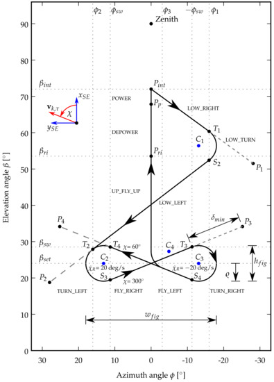
Figure 4.
Flight-path planner (FPP) for the entire pumping cycle, including the four-step planner for down-loop figure-of-eight maneuvers: first, turn left, then steer towards attractor point , then turn right, and finally steer towards attractor point [12].
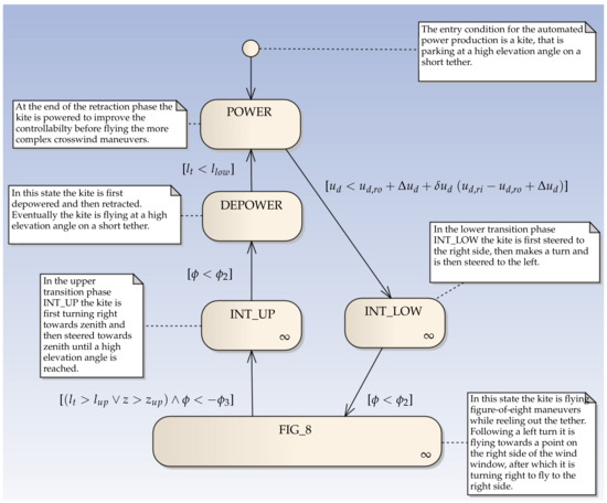
Figure 5.
Finite state diagram for the states of the high-level controller for fully automated power production.
The downloop flight maneuvers are (we distinguish between downloops and uploops depending on the direction of flight during the turning maneuvers along the outer parts of the figure of eight. While downloops lead to a more equalized power profile during the traction phase, uploops are generally considered to be more safe) flight maneuvers are constructed in four steps, as shown in Table 1 and Figure 6. The flight maneuver starts from the initial position of the kite with a left turn (substate TURN_LEFT). During the turn, the set value , computed from theturn rate law given by Equation (8), is used. When reaching the switch condition , the turning maneuver is stopped, and the kite starts flying to the right towards attractor point (substate FLY_RIGHT). On this segment of the figure of eight, the kite is steered by the PID controller, as described in Section 2.3. A relatively large offset of is needed to compensate for the time delay s between the command to stop turning and the kite actually stopping to turn [12]. For clarity of illustration, we use a value of in Figure 4 and Figure 7a, such that the circular-path segments with constant turn rate directly connect with the straight-path segments with constant course angle . When reaching the switch condition , the kite starts a right turn (substate TURN_RIGHT). During the turn, the set value computed from the turn rate law is used. When reaching the switch condition , the turning maneuver is stopped, and the kite starts flying to the left towards attractor point (substate FLY_LEFT). On this segment of the figure of eight, the kite is again steered by the PID controller. When reaching the switch condition , a new figure-of-eight maneuver is started with the kite entering a left turn (substate TURN_LEFT).

Table 1.
Finite substates of the figure-of-eight flight path planner [28]. Set value for position is used only when the proportional-integral-derivative (PID) controller is active. Set value for the turn rate is used only when the PID is inactive.
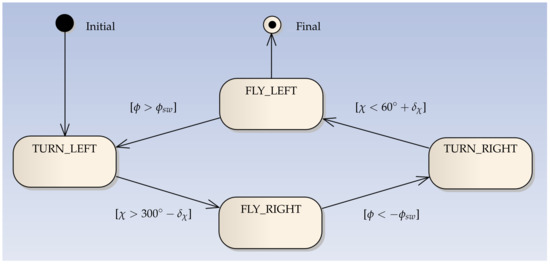
Figure 6.
Finite substate diagram showing the substate and the transitional condition of the figure-of-eight controller.
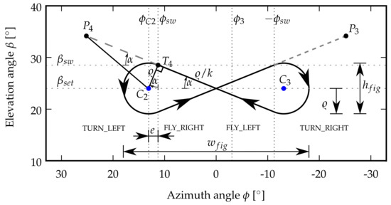
As illustrated in Figure 4, the geometry of the figure-of-eight flight path is defined by the angular width and height , and the minimal attractor point distance , which is defined as the arc length on the unit sphere between the kite position and the current attractor point, at which the kite stops flying towards this attractor point and starts to make a turn. If the aforementioned parameters are specified, then , , and can be calculated by the FPP. The motion of the kite on the planned trajectory is described by the tangential velocity of the kite , defined by Equation (2), and the turning radius, defined as
The rate of change of the course angle required to fly a turn with radius R is calculated as
where the angular velocity of the kite with respect to the origin is given by Equation (6). The turning radius , as defined by Equation (9), is an arc length on the unit sphere, while the radius of curvature R, as used in Equation (10), is a distance in Cartesian space. For practically relevant figure-of-eight maneuvers with small turning radius, we can use the following approximation:
The value of can be calculated from
Then, the switch values and of the azimuth and elevation angles can be calculated from Equations (13) and (14) by combining the circle segment of the left turn with the tangent.
The slope of the line segment towards can be calculated from
Solving for the attractor points and , we obtain
2.3. Flight Path Control (FPC)
The FPC uses the attractor points and to guide the kite during the FLY_RIGHT and FLY_LEFT substates of the figure-of-eight maneuver. The required course angle is calculated from the set values of the elevation and azimuth angles using great circle navigation [32]
Since the kite model is designed as a SISO system, it has just one error signal that comes from the difference between the actual course angle of the kite, determined by integration of Equation (8), and the set value for the course angle, given by Equation (20). This error signal is fed into a PID controller that uses the relative steering input to align the tangential velocity of the kite with the planned flight direction.
The kite is steered along the turns of the figure-of-eight maneuver using a feed-forward controller with the set value , computed from the turn rate law given by Equation (8), to fly a turn with radius R (or in - space). This set value is used as input of a nonlinear-dynamic-inversion (NDI) block to calculate the relative steering action that is required to fly the respective turn. The functions used by the NDI block are detailed in [12].
3. System Identification (SI) Using Plackett’s Algorithm
The aim of the SI algorithm is to estimate the system parameters during automatic flight using sensor data. Therefore, it is required to update the parameters in real time by analyzing the history of the control action and the course angle [28]. There are several techniques for SI. In this paper, we used Plackett’s algorithm [29,30] as a technique to update the dynamics of the system. This specific algorithm has the advantage of rapidly acquiring the system parameters without iterations, has no singularity, and the implementation on a microcontroller is simple and can be used for real-time processing for flight tests.
The algorithm is based on the minimization of the mean square error (MSE) of the course angle , as defined by
where k is total number of time steps in the discrete time process, are the measured data for time step r, and the estimated value determined by the SI algorithm. The open-loop transfer function (TF) of the kite was derived in [28] and was used as a case study. The control action is denoted as , and the course angle is denoted as . The block diagram of the SI algorithm and adaptive control system is illustrated in Figure 8.
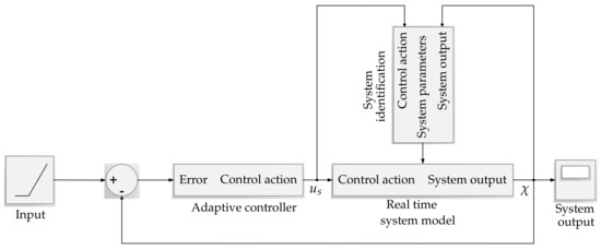
Figure 8.
Block diagram of System Identification (SI) algorithm and adaptive control system.
The SI algorithm predicts the course angle and updates the coefficients and of the open-loop TF. Following that, the adaptive control updates its gains to stabilize the kite, as described in Section 4. The simulation results presented in Section 5 were calculated on the basis of the SI algorithm. This required to get the values of the control action and kite course angle as input for the algorithm to estimate the coefficients and for two different flight conditions. Finally, these simulation results were compared with results of the simplified model using a PID controller.
In Section 6, the SI algorithm was implemented in a different way. It utilizes the relative steering action and course angle measured during a physical flight test of the TU Delft V3 kite to identify the coefficients of the open loop TF. Neither the simplified model presented in Section 2 nor any controller algorithms were used in this process. The open-loop TF for the kite in z-form [33] can be approximated as
where and are considered as second-order polynomial equations in z-form:
The coefficients and vary with time because of the change in the system dynamics. The kite is also exposed to a time-varying apparent wind speed that is not available in real time during flight. Substituting Equations (23) and (24) into Equation (22), we obtain
Which can be rewritten in difference form as
or reformulated as a matrix expression
where
From Equation (21), the MSE can be written as
The objective of the SI algorithm is to obtain the values of the coefficient matrix that minimize the MSE. From the derivation, these values can be calculated as
where is a square matrix, such that
From Equation (32), we obtain
Such that Equation (31) can now be rewritten as
Equation (33) can be rewritten as
In Equation (37), the term is unknown; thus, we can apply the Lemma formula [34] to Equation (36) to arrive at
Thus, the unknown coefficients and have to be calculated in every time step as to update the estimated course angle given in Equation (26). The following calculation steps are required to obtain these parameters. First, the matrix is initialized with large positive numbers on the leading diagonal and zeroes on the off-diagonal elements. The matrix must be populated with initial parameters close to the model. Then, the simulation results of the SI algorithm are obtained with the following steps:
4. Robust Pole-Placement Controller
The aim of this section is to design an adaptive control algorithm to stabilize the simplified kite model of Section 2. The control gains are updated with the SI algorithm described in the previous section, which makes the controller more robust compared to the classical control technique implemented in [12]. Moreover, the controller can simply be implemented on a microcontroller and installed in the KCU for autonomous operation of the kite. The closed-loop TF of the system in z-form is defined as
where is the open-loop TF of the system given by Equation (22), and is the controller TF, as defined by
The next step is to calculate the controller functions and , and their order [35]. We assume that these functions can be expressed as polynomials of order n:
The orders and of and can be calculated from Equations (45) and (46). They are related to the orders and of the open-loop TF, as follows.
Then, the characteristic equation of the closed-loop TF can be rewritten as
Equation (49) is the characteristic equation of the closed-loop TF. By solving this equation, we are able to tune the system behavior, i.e. the time constant and steady-state error. The orders of the controller polynomials are calculated from the order of the open-loop TF. The required characteristics of our system is to place the poles of the closed-loop TF at certain positions so as to achieve system stability and robustness. We introduce the following equation:
where is a polynomial function that contains the controller characteristics, and is the polynomial function that is responsible for stabilizing the order of the equation. The controller parameters and can be determined by comparing the coefficients of the same order in Equation (50). In our design, the poles of the closed-loop TF in the z-form are , , and .
The sampling time used during the simulation was s. Thus, the chosen poles can be rewritten as
The characteristic equation of our model is a third-order polynomial. We applied Jury’s stability test [36], which is similar to the Routh–Hurwitz stability criterion used for continuous-time systems, and found that all roots were located inside the unit circle, which is a condition for stability. Although Jury’s stability test can be applied to characteristic equations of any order, its complexity increases for higher-order systems.
Finally, we have three unknowns, , and . By substituting Equation (51) into Equation (50), we obtaine three equations that we combine into a Sylvester matrix [37], as defined by the following equation:
The controller parameters and are dependent on the parameters of the SI algorithm. In the following section, we show that the robust pole placement controller and SI algorithm increase the flight dynamic stability of the kite when exposed to sudden changes of the apparent wind speed.
5. Simulation Results
In this section, we present simulation results using the model and algorithms described in Section 2, Section 3 and Section 4. We compared the results of a classical (PID) controller implemented in [12] with the adaptive control demonstrated in Section 4 to show the capability of the adaptive control to increase the stability of the kite flight. Both controllers use the simplified kite model derived in Section 2. We investigated the flight dynamic responses of the kite for the two wind speed signals shown in Figure 9 and Figure 10. Flight condition I is discussed in Section 5.1, while flight condition II, which is characterized by a much higher frequency, is discussed in Section 5.2.
Figure 9.
Time history for wind speed during flight condition I.
Figure 10.
Time history for wind speed during flight condition II.
5.1. Flight Condition I
Flight condition I is based on the wind speed signal illustrated in Figure 9. The fluctuations affect the flight dynamics of the kite, as described by the model presented in Section 2. The SI algorithm derived in Section 3 generates the values of the coefficients and , shown in Figure 11 and Figure 12. The resulting figure-of-eight trajectory is illustrated in Figure 13, calculated using the simple model and the classical controller presented in Section 2.
Figure 11.
Time history of TF coefficients and .

Figure 12.
Time history of TF coefficients and .
Figure 13.
Trajectory computed on the basis of the classical flight controller for flight time of 70 s.
The figure-of-eight trajectory illustrated in Figure 14 was calculated on the basis of the SI algorithm and adaptive controller described in Section 3 and Section 4. The controller parameters are updated in real time, accounting for varying parameters , and , as shown in Figure 15 and Figure 16, which are, in turn, updated from the varying TF coefficients and .
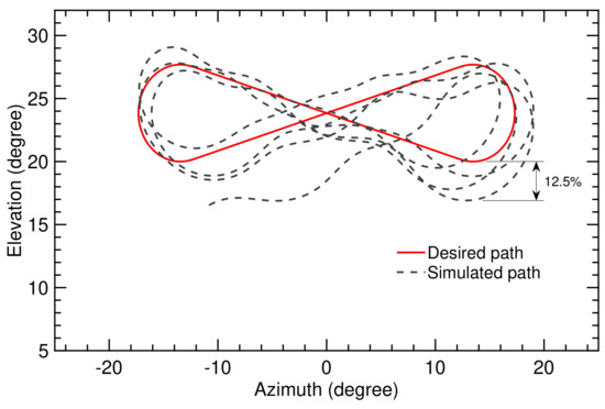
Figure 14.
Trajectory computed on the basis of the SI algorithm and adaptive controller for flight time of 70 s.
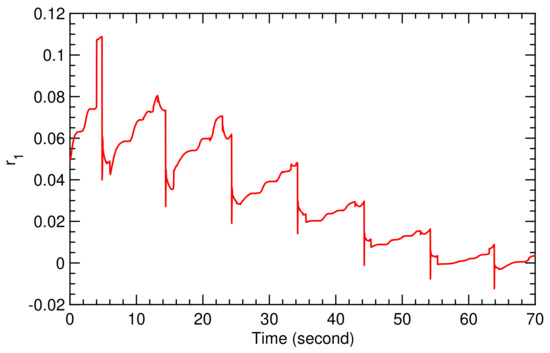
Figure 15.
Time history of controller parameter for flight condition I.
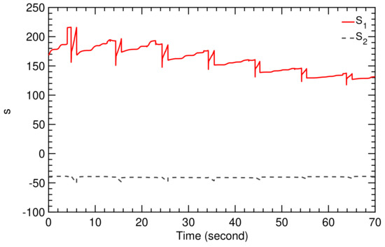
Figure 16.
Time history of controller parameters and for flight condition I.
Figure 17 shows a very close fit between the measured course angle from the model and the estimated value from the SI algorithm. This accuracy was achieved for a sampling time of s, which is very short for this type of application.
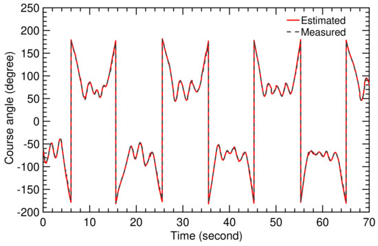
Figure 17.
Time history of measured and estimated values of course angle.
To assess the tracking performance of the different control approaches, we used the deviation between the computed and the planned flight paths. From the several options to quantify this deviation, in this study we chose the elevation angle. The difference in elevation angle is a suitable measure to quantify the operational stability of the kite because if this difference increases too much, the wing can experience aerodynamic stall. Therefore, the designed control parameters have to be carefully chosen to keep the deviation of the elevation angle below a certain limit.
Figure 13 indicates that the deviation between simulated and desired paths depends on the position along the path. The error increases after performing the turning maneuver. The maximal deviation over the total simulation time was (). Using the SI algorithm with the adaptive controller, the maximal deviation was (), as depicted in Figure 14. This was acceptable for maintaining a stable flight.
5.2. Flight Condition II
Flight condition II is based on the wind speed signal illustrated in Figure 10, which is characterized by fluctuations at much higher frequency compared to flight condition I. For this reason, flight condition II is much more demanding for the controller, which we can see from the values of the TF coefficients and , displayed in Figure 18 and Figure 19.
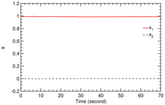
Figure 18.
Time history of TF coefficients and .
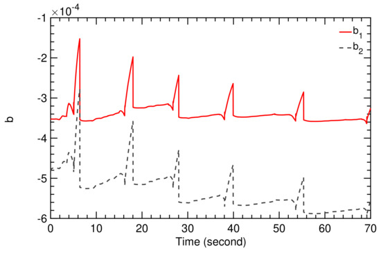
Figure 19.
Time history of TF coefficients and .
The order of the coefficients and in Figure 12 and Figure 19 is different because the different frequencies of the wind speed fluctuations affected the flight dynamic model of the kite, which was then detected by the SI algorithm.
The computed trajectories are illustrated in Figure 20 and Figure 21. Figure 20 shows that the figure-of-eight motion of the kite progressively drops towards lower elevation angles, while Figure 21 shows that the figure-of-eight motion stays in the vicinity of the set value . From this we conclude that the classical flight controller is not able to maintain a stable flight operation for flight condition II, while the combination of the SI algorithm and adaptive controller is.
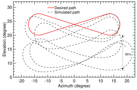
Figure 20.
Trajectory computed on the basis of classical flight controller for flight time of 70 s.
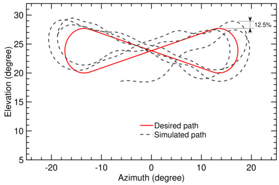
Figure 21.
Trajectory computed on the basis of the SI algorithm and adaptive controller for flight time of 70 s.
To explain why flight condition II leads to an unstable flight operation we look at the differences of the two control approaches used in the simulation. The classical flight controller is based on a PID controller with constant gains. While this is suitable for flight condition I, it was not able to cope with the dynamic reaction of the model to the more rapidly fluctuating wind speed of flight condition II. In contrast to the classical controller, the combination of the SI algorithm and adaptive controller was able to manage this dynamic reaction because the TF coefficients and and controller parameters , and are updated in real time, as shown in Figure 18, Figure 19, Figure 22 and Figure 23, respectively.
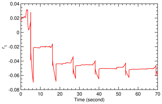
Figure 22.
Time history of controller parameter for flight condition II.
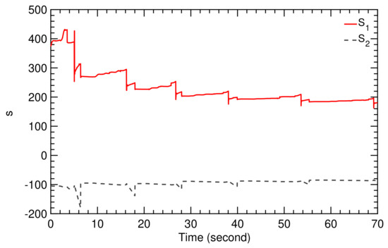
Figure 23.
Time history of controller parameters and for flight condition II.
Figure 24 shows again a very close fit between measured and estimated course angle, which demonstrates the performance of the SI algorithm for a strongly fluctuating wind speed.
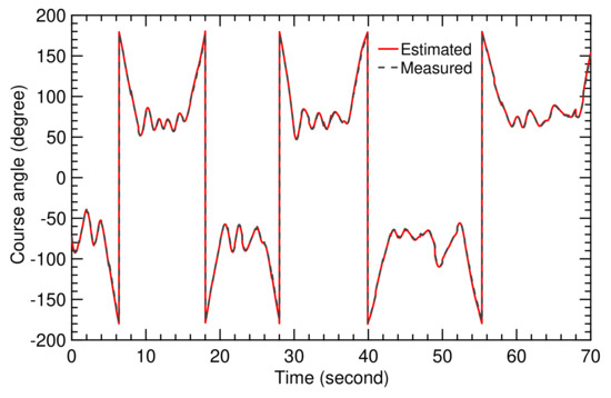
Figure 24.
Time history of measured and estimated course angles.
As indicated by Figure 20, the deviation of the computed elevation angle from the planned elevation angle increases steadily along the trajectory until it reaches its maximum () with the last turn. This maximal deviation is three times the maximal deviation for flight condition I (see Figure 13). Figure 21 shows a maximal deviation of (), which is almost the same as for flight condition I (see Figure 14).
6. Experimental Results
In this section, we apply the SI algorithm to data that were recorded during a flight test of the 20 kW kite power system of Delft University of Technology. The objective was to derive a mathematical model of the kite power system directly from measurement data, omitting the use of an underlying system model with many simplifying assumptions. As a result, we implicitly considered the effects of the fluctuating wind velocity (magnitude and direction) and deforming wing due to a varying aerodynamic load distribution and actuation of the bridle line system. In Section 6.1, we describe the configuration of the kite power system during the selected flight test. In Section 6.2, we use the SI algorithm to derive a mathematical model of the kite power system.
6.1. System Configuration
The flight test was performed by the research group on 25 October 2012 [38], using the TU Delft V3 kite that is illustrated in Figure 3 and in more detail in Figure 25.
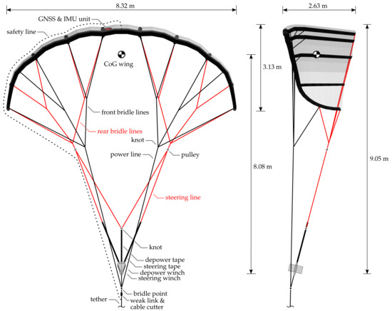
Figure 25.
TU Delft V3 kite in front (left) and side view (right) [38]. KCU is displayed without the exterior foam shell and the attached small wind turbine for supplying onboard power.
This specific kite has a total wing surface area of 25 m, and is a customized and scaled-up derivative of the Hydra kite, which is a commercially available surf kite with a total wing surface area of 14 m. The TU Delft V3 kite consists of a flexible membrane wing, a bridle line system, and a small remote-controlled cable robot, the KCU. The wing is designed as a leading edge inflatable (LEI) tube kite, using an inflated tubular frame to collect the distributed aerodynamic load acting on the canopy and transmit this load to the bridle lines. The front bridle lines directly attach to the tether, transmitting the major part of the forces, while the KCU connects the two branches of the rear bridle lines to the tether. The integrated steering and depower winches can adjust the lengths of the steering and depower tapes to steer the wing and to adapt its angle-of-attack, respectively. The angle-of-attack is decreased during the reel-in phase to minimize the energy required to retract the kite. There are two software algorithms to control the system: the first algorithm is for maintaining figure-of-eight maneuvers during the reel-out phase while the second algorithm is for the reel-in phase. A detailed description of the different functional components of the kite power system is given in [5,8,39].
6.2. System Identification
The results presented in this section are based on two consecutive pumping cycles that start 2615 s after kite launch at 15:13:41 (hh:mm:ss) [38]. Each pumping cycle consists of 110 s of tether reel-out, followed by 70 s of tether reel-in. The flight motion of the kite is affected by a variety of parameters, such as tether force, reeling speed, KCU steering actuation, and the dynamics of the drum-generator module on the ground. Therefore, the SI algorithm described in Section 3 was used to directly determine the SI parameters of the kite system using experimental measurements. We determined the course angle from the recorded flight data by using the attitude sensors and relative steering action . These data were sufficient for the SI algorithm to derive the TF coefficients and in real time.
The recorded flight path of the kite for the two consecutive pumping cycles is illustrated in Figure 26 and Figure 27. The kite starts at an altitude of 240 m and subsequently dives down to the minimal altitude of 115 m to start a first sequence of figure-of-eight maneuvers around an average elevation angle of . During these maneuvers, the azimuth angle varies between and , the tether reels out and the altitude progressively increases. After around 100 s, the figure-of-eight maneuvers are discontinued and the tether is reeled in. In this phase, the kite passes through a maximal azimuth angle of , a maximal elevation angle of , and climbes to the maximal altitude of 315 m before again diving down to around 115 m to start a second sequence of figure-of-eight maneuvers. Flying to large azimuth and elevation angles is a second technique to depower the kite, and it was used in this specific test flight in addition to reducing the angle of attack of the wing. Towards the end of the second reel-in phase, the kite reaches the maximal elevation angle of almost at a constant azimuth angle of , climbing to the maximal altitude of 365 m.
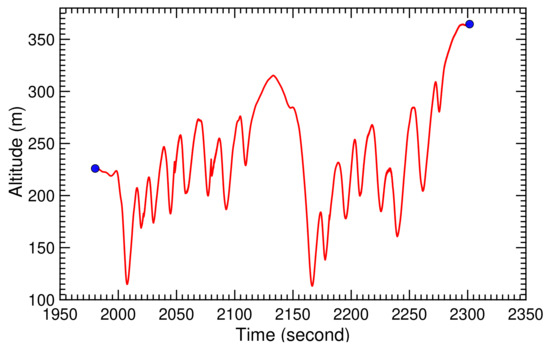
Figure 26.
Recorded kite altitude for two pumping cycles. The origin of the time scale in this and subsequent time-history diagrams is not synchronized with the launch event.
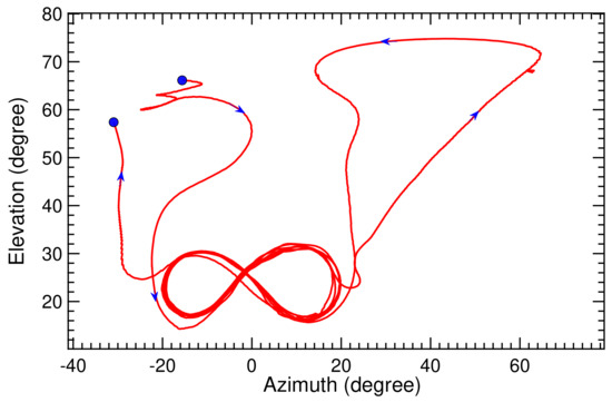
Figure 27.
Recorded azimuth and elevation angles for two pumping cycles.
The recorded ground wind speed during the two selected pumping cycles is shown in Figure 28, the recorded relative steering action in Figure 29, and the recorded measured course angle in Figure 30. From these, we calculated the TF coefficients and , displayed in Figure 31 and Figure 32. The time-history diagrams reveal strong variations of the coefficients at 1990, 2110, and 2280 s. These variations coincide with the transitions between reel-in and reel-out phases, and demonstrate the capability of the SI algorithm to adjust to the system dynamics even when rapidly changing operating modes.
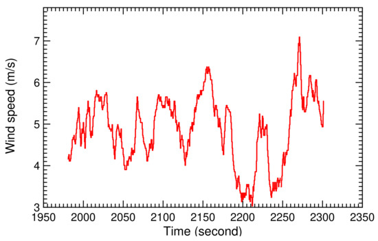
Figure 28.
Recorded ground wind speed for two pumping cycles.
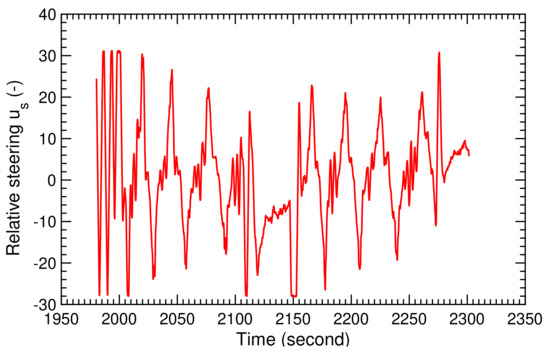
Figure 29.
Recorded relative steering action for two pumping cycles.
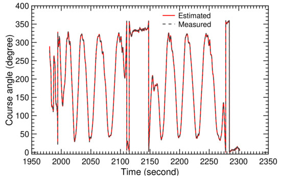
Figure 30.
Measured and estimated course angle for two pumping cycles.
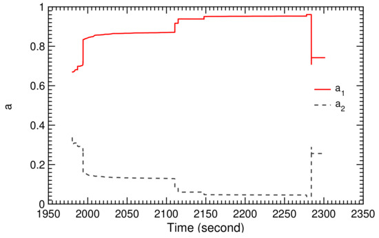
Figure 31.
Calculated TF coefficients and for two pumping cycles.
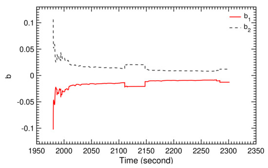
Figure 32.
Calculated TF coefficients and for two pumping cycles.
The open-loop TF of the TU Delft V3 kite was obtained from Equation (25) using the calculated values of the TF coefficients displayed in Figure 31 and Figure 32. The resulting correlation between relative steering action and course angle of the kite can be used for the planning and control of autonomous flight operation. The correlation was also used in Figure 30 to estimate the course angle using the recorded relative steering action , displayed in Figure 29. The close fit between measured and estimated course angle indicates the capability of the chosen SI algorithm to identify system parameters without any singularity in a very short sampling time.
The recorded tether force measured at the ground is shown in Figure 33. One can clearly distinguish the reel-out phases with an average tether force of 3000 N and the reel-in phases with an average tether force of 700 N. The strong oscillations during the reel-out phase are induced by the figure-of-eight motion, because the tether force is proportional to [40], and the wind speed fluctuations at the kite position [13].
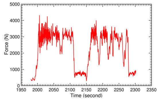
Figure 33.
Recorded tether force for two pumping cycles.
7. Conclusions
In this paper, we studied the flight control of a tethered flexible-membrane kite used for airborne wind energy harvesting in pumping cycles. Specifically, we investigated the figure-of-eight maneuvers of the kite during the energy-generating reel-out phase. Following the development of a simplified kite system model and a flight path planning algorithm, we compared a classical PID controller using fixed gains with an adaptive controller that uses a system identification algorithm to adjust the controller parameters in real time. The performance of the two different control approaches was assessed on the basis of two flight conditions that were characterized by different fluctuation frequencies of wind speed. We found that the classical control was not able to cope with rapidly fluctuating wind speed. On the other hand, the combination of adaptive control and SI algorithm was more robust, and was able to handle more severely fluctuating wind speed and varying flight dynamic behavior of the kite. The enhanced stability was a result of the real-time tuning of the control gains at every integration time step to the varying SI parameters. Then, the SI algorithm was successfully applied to recorded measurement data of a test flight of a 20 kW kite power system, equipped with a kite of 25 m wing surface area. Despite the uncertainty of the wind velocity in magnitude and direction, and the dynamic response of the deformable membrane wing, it was possible to successfully derive the SI parameters of the system for different operating phases, such as reel-in and reel-out. The results suggest that the combination of adaptive controller and SI algorithm is well-suited for robust path control of a tethered membrane kite flying in a fluctuating wind field, and transitioning through different operating phases. As a next step for this research, we aim to implement the adaptive controller with the experimental hardware to demonstrate its performance in a flight-test campaign.
Author Contributions
Conceptualization and methodology, T.N.D., U.F., R.S., S.Y.; software, T.N.D., U.F.; validation, T.N.D., M.A.R.; writing–original draft preparation, T.N.D., U.F.; writing–review and editing, T.N.D., R.S.; supervision and funding acquisition, R.S., S.Y. All authors have read and agree to the published version of the manuscript.
Funding
R.S. was supported by the H2020-ITN project AWESCO funded by the European Union’s Horizon 2020 research and innovation program under the Marie Skłodowska-Curie grant, agreement no. 642682.
Acknowledgments
The authors are grateful to Kitepower B.V. (http://www.kitepower.nl) for sharing their expertise on simulation and greatly enhancing the practical relevance of the research.
Conflicts of Interest
The authors declare no conflict of interest.
Nomenclature
| Latin Symbol | ||
| A | denominator polynomial of open-loop TF | - |
| , , , | coefficients of the open-loop TF | - |
| B | numerator polynomial of open-loop TF | - |
| , , | adaptive control parameters | - |
| gravity-sensitivity coefficient of turn rate law | rad.m/s | |
| steering-sensitivity coefficient of turn rate law | rad/m | |
| steering offset of turn rate law | - | |
| open-loop TF of model in z-domain | - | |
| closed-loop TF of model in z-domain | - | |
| angular height of figure-of-eight maneuver | rad | |
| tether length | m | |
| , | angular reference positions for FPP | rad |
| order of R-polynomial | - | |
| R | numerator polynomial of control TF | - |
| r | radial coordinate of kite | m |
| order of S-polynomial | - | |
| S | denominator polynomial of control TF | - |
| system input defined as in z-domain | - | |
| relative depower action | - | |
| relative steering action | - | |
| horizontal wind velocity at reference height | m/s | |
| , , | body-fixed kite reference frame | - |
| , , | small earth reference frame | - |
| , , | wind reference frame | - |
| estimated course angle obtained from system identification in z-domain | rad | |
| measured course angle obtained from sensor | rad | |
| backward shift operator in z-domain | - | |
| Greek Symbol | ||
| kite elevation angle | rad | |
| elevation angle to switch flight mode | rad | |
| kite course angle | ||
| rate of change of course angle | rad/s | |
| rate of change of course angle to fly a turn with radius R | rad/s | |
| set value for course angle | rad | |
| minimal angular attractor point distance | rad | |
| angular width of figure-of-eight maneuver | rad | |
| reference value of angular speed | rad/s | |
| kite azimuth angle | rad | |
| azimuth angle at point | rad | |
| set value of azimuth angle | rad | |
| azimuth angle to switch flight mode | rad | |
| kite heading angle | rad | |
| kite turn rate | rad/s | |
| turn radius of kite point trajectory | rad | |
| Vectors and Matrices | ||
| angular velocity of kite point with respect to origin | rad/s | |
| kite position in angular co-ordinates(, ) | rad | |
| covariance matrix of estimated error | - | |
| last vector estimated using least-squares estimation algorithm | - | |
| apparent wind speed | m/s | |
| kite velocity | m/s | |
| radial kite velocity component | m/s | |
| tangential kite velocity component | m/s | |
| data of old measurement of course angle and control action | - | |
| measured course angle obtained from sensor | rad | |
| Abbreviation | ||
| AWE | Airborne Wind Energy | |
| FPC | Flight Path Control | |
| FPP | Flight Path Planner | |
| HAWT | Horizontal Axis Wind Turbines | |
| KCU | Kite Control Unit | |
| LEI | Leading Edge Inflatable | |
| MSE | Mean Square Error | |
| NDI | Nonlinear Dynamic Inversion | |
| NMPC | Nonlinear Model Predictive Control | |
| PID | Proportional-Integral-Derivative | |
| SI | System Identification | |
| SISO | Single-Input Single-Output | |
| TF | Transfer Function | |
| TU Delft | Delft University of Technology | |
References
- Ahrens, U.; Diehl, M.; Schmehl, R. (Eds.) Airborne Wind Energy; Green Energy and Technology; Springer: Berlin/Heidelberg, Germany, 2013. [Google Scholar] [CrossRef]
- Cherubini, A.; Papini, A.; Vertechy, R.; Fontana, M. Airborne Wind Energy Systems: A review of the technologies. Renew. Sustain. Energy Rev. 2015, 51, 1461–1476. [Google Scholar] [CrossRef]
- Schmehl, R. (Ed.) Airborne Wind Energy—Advances in Technology Development and Research; Green Energy and Technology; Springer: Singapore, 2018. [Google Scholar] [CrossRef]
- Lago, J.; Erhard, M.; Diehl, M. Warping model predictive control for application in control of a real airborne wind energy system. Control Eng. Pract. 2018, 78, 65–78. [Google Scholar] [CrossRef]
- Van der Vlugt, R.; Peschel, J.; Schmehl, R. Design and experimental characterization of a pumping kite power system. In Airborne Wind Energy; Ahrens, U., Diehl, M., Schmehl, R., Eds.; Green Energy and Technology; Springer: Berlin/Heidelberg, Germany, 2013; Chapter 23; pp. 403–425. [Google Scholar] [CrossRef]
- Goldstein, L. Airborne wind energy conversion systems with ultra high speed mechanical power transfer. In Airborne Wind Energy; Ahrens, U., Diehl, M., Schmehl, R., Eds.; Green Energy and Technology; Springer: Berlin/Heidelberg, Germany, 2013; Chapter 13; pp. 235–247. [Google Scholar] [CrossRef]
- Diehl, M.; Leuthold, R.; Schmehl, R. (Eds.) The International Airborne Wind Energy Conference 2017: Book of Abstracts; University of Freiburg: Freiburg, Germany; Delft University of Technology: Delft, The Netherlands, 2017. [Google Scholar] [CrossRef]
- Van der Vlugt, R.; Bley, A.; Schmehl, R.; Noom, M. Quasi-steady model of a pumping kite power system. Renew. Energy 2019, 131, 83–99. [Google Scholar] [CrossRef]
- De Wachter, A. Power from the skies: Laddermill takes airborne wind energy to new heights. Leonardo Times J. Soc. Aerosp. Eng. Stud. VSV Leonardo da Vinci 2010, 10, 18–20. [Google Scholar]
- Bosch, A.; Schmehl, R.; Tiso, P.; Rixen, D. Dynamic nonlinear aeroelastic model of a kite for power generation. J. Guid. Control Dyn. 2014, 37, 1426–1436. [Google Scholar] [CrossRef]
- Fechner, U.; van der Vlugt, R.; Schreuder, E.; Schmehl, R. Dynamic model of a pumping kite power system. Renew. Energy 2015, 83, 705–716. [Google Scholar] [CrossRef]
- Fechner, U. A Methodology for the Design of Kite-Power Control Systems. Ph.D. Thesis, Delft University of Technology, Delft, The Netherlands, 2016. [Google Scholar] [CrossRef]
- Fechner, U.; Schmehl, R. Flight Path Planning in a Turbulent Wind Environment. In Airborne Wind Energy—Advances in Technology Development and Research; Schmehl, R., Ed.; Green Energy and Technology; Springer: Singapore, 2018; Chapter 15; pp. 361–390. [Google Scholar] [CrossRef]
- Breukels, J.; Schmehl, R.; Ockels, W. Aeroelastic Simulation of Flexible Membrane Wings based on Multibody System Dynamics. In Airborne Wind Energy; Ahrens, U., Diehl, M., Schmehl, R., Eds.; Green Energy and Technology; Springer: Berlin/Heidelberg, Germany, 2013; Chapter 16; pp. 287–305. [Google Scholar] [CrossRef]
- Bosch, A.; Schmehl, R.; Tiso, P.; Rixen, D. Nonlinear Aeroelasticity, Flight Dynamics and Control of a Flexible Membrane Traction Kite. In Airborne Wind Energy; Ahrens, U., Diehl, M., Schmehl, R., Eds.; Green Energy and Technology; Springer: Berlin/Heidelberg, Germany, 2013; Chapter 17; pp. 307–323. [Google Scholar] [CrossRef]
- Oehler, J.; Schmehl, R. Aerodynamic characterization of a soft kite by in situ flow measurement. Wind Energy Sci. 2019, 4, 1–21. [Google Scholar] [CrossRef]
- Erhard, M.; Strauch, H. Theory and Experimental Validation of a Simple Comprehensible Model of Tethered Kite Dynamics Used for Controller Design. In Airborne Wind Energy; Ahrens, U., Diehl, M., Schmehl, R., Eds.; Green Energy and Technology; Springer: Berlin/Heidelberg, Germany, 2013; Chapter 8; pp. 141–165. [Google Scholar] [CrossRef]
- Fagiano, L.; Milanese, M.; Piga, D. Optimization of airborne wind energy generators. Int. J. Robust Nonlinear Control 2012, 22, 2055–2083. [Google Scholar] [CrossRef]
- Erhard, M.; Horn, G.; Diehl, M. A quaternion-based model for optimal control of an airborne wind energy system. ZAMM-J. Appl. Math. Mech./Zeitschrift für Angewandte Mathematik und Mechanik 2017, 97, 7–24. [Google Scholar] [CrossRef]
- Gros, S.; Zanon, M.; Diehl, M. A relaxation strategy for the optimization of Airborne Wind Energy systems. In Proceedings of the 2013 European Control Conference (ECC), Zurich, Switzerland, 17–19 July 2013; pp. 1011–1016. [Google Scholar]
- Rawlings, J.B.; Amrit, R. Optimizing process economic performance using model predictive control. In Nonlinear Model Predictive Control; Magni, L., Raimondo, D.M., Allgöwer, F., Eds.; Lecture Notes in Control and Information Sciences; Springer: Berlin/Heidelberg, Germany, 2009; Volume 384, pp. 119–138. [Google Scholar] [CrossRef]
- Winter, M.; Schmidt, E.; Silva de Oliveira, R. An open-source software platform for AWE systems. In Book of Abstracts of the International Airborne Wind Energy Conference 2017; Diehl, M., Leuthold, R., Schmehl, R., Eds.; University of Freiburg: Freiburg, Germany; Delft University of Technology: Delft, The Netherlands, 2017; p. 140. Available online: http://awec2017.com/images/posters/Poster_Araujo.pdf (accessed on 28 January 2020).
- Sieg, C.; Gehrmann, T.; Bechtle, P.; Zillmann, U. AWEsome: An Affordable Standardized Open-Source Test Platform for AWE Systems. In Book of Abstracts of the International Airborne Wind Energy Conference 2017; Diehl, M., Leuthold, R., Schmehl, R., Eds.; University of Freiburg: Freiburg, Germany; Delft University of Technology: Delft, The Netherlands, 2017; p. 24. Available online: http://awec2017.com/images/posters/Poster_Sieg.pdf (accessed on 28 January 2020).
- Dunker, S. Tether and Bridle Line Drag in Airborne Wind Energy Applications. In Airborne Wind Energy; Schmehl, R., Ed.; Green Energy and Technology; Springer: Singapore, 2018; pp. 29–56. [Google Scholar] [CrossRef]
- Rapp, S.; Schmehl, R. Vertical takeoff and landing of flexible wing kite power systems. J. Guid. Control Dyn. 2018, 41, 2386–2400. [Google Scholar] [CrossRef]
- Fagiano, L.; Zgraggen, A.U.; Morari, M.; Khammash, M. Automatic crosswind flight of tethered wings for airborne wind energy: Modeling, control design and experimental results. IEEE Trans. Control Syst. Technol. 2014, 22, 1433–1447. [Google Scholar] [CrossRef]
- Alvin, K.F.; Park, K. Second-order structural identification procedure via state-space-based system identification. AIAA J. 1994, 32, 397–406. [Google Scholar] [CrossRef]
- Dief, T.N.; Fechner, U.; Schmehl, R.; Yoshida, S.; Ismaiel, A.M.; Halawa, A.M. System identification, fuzzy control and simulation of a kite power system with fixed tether length. Wind Energy Sci. 2018, 3, 275–291. [Google Scholar] [CrossRef]
- Plackett, R.L. Some theorems in least squares. Biometrika 1950, 37, 149–157. [Google Scholar] [CrossRef] [PubMed]
- Dutton, K.; Thompson, S.; Barraclough, B. Adaptive and self-tunning control. In The Art of Control Engineering; Addison-Wesley Longman Publishing Co., Inc.: Reading, MA, USA, 1997; Chapter 11; pp. 560–582. [Google Scholar]
- Jehle, C.; Schmehl, R. Applied tracking control for kite power systems. J. Guid. Control Dyn. 2014, 37, 1211–1222. [Google Scholar] [CrossRef]
- Baayen, J.H.; Ockels, W.J. Tracking control with adaption of kites. IET Control Theory Appl. 2012, 6, 82–191. [Google Scholar] [CrossRef]
- Burns, R. Advanced Control Engineering, 1st ed.; Butterworth-Heinemann: London, UK, 2001. [Google Scholar] [CrossRef]
- Hager, W.W. Updating the inverse of a matrix. SIAM Rev. 1989, 31, 221–239. [Google Scholar] [CrossRef]
- Bobál, V.; Böhm, J.; Fessl, J.; Machácek, J. Digital Self-Tuning Controllers: Algorithms, Implementation And Applications; Springer: London, UK, 2005. [Google Scholar]
- Ibrahim, D. System Stability. In Microcontroller Based Applied Digital Control; Ibrahim, D., Ed.; Wiley Online Library: New Delhi, India, 2006; Chapter 8; pp. 187–211. [Google Scholar] [CrossRef]
- Lee, S.G.; Vu, Q.P. Simultaneous solutions of Sylvester equations and idempotent matrices separating the joint spectrum. Linear Algebra Its Appl. 2011, 435, 2097–2109. [Google Scholar] [CrossRef]
- Schmehl, R.; Fechner, U. Kite Power Flight Data 2011–2015; Data Set; 4TU. Centre for Research Data: Delft, The Netherlands, 2020. [Google Scholar] [CrossRef]
- Salma, V.; Friedl, F.; Schmehl, R. Improving Reliability and Safety of Airborne Wind Energy Systems. Wind Energy 2020, 23, 340–356. [Google Scholar] [CrossRef]
- Schmehl, R.; Noom, M.; van der Vlugt, R. Traction Power Generation with Tethered Wings. In Airborne Wind Energy; Ahrens, U., Diehl, M., Schmehl, R., Eds.; Green Energy and Technology; Springer: Berlin/Heidelberg, Germany, 2013; Chapter 2; pp. 23–45. [Google Scholar] [CrossRef]
© 2020 by the authors. Licensee MDPI, Basel, Switzerland. This article is an open access article distributed under the terms and conditions of the Creative Commons Attribution (CC BY) license (http://creativecommons.org/licenses/by/4.0/).