Optimal Price Based Demand Response of HVAC Systems in Commercial Buildings Considering Peak Load Reduction

Abstract

Electric utility companies (EUCs) play an intermediary role of retailers between wholesale market and end-users, maximizing their profits. Retail pricing can be well deployed with the support of EUCs to promote demand response (DR) programs for heating, ventilating, and air-conditioning (HVAC) systems in commercial buildings. This paper proposes a pricing strategy to help EUCs and building operators achieve an optimal DR of price-elastic HVAC systems, considering peak load reduction. The proposed strategy is implemented by adopting a bi-level decision model. The nonlinear thermal response of an experimental building room is modeled using piecewise linear equations, which helps convert the bi-level model to the single-level model. The pricing strategy is implemented considering a time-of-use (TOU) pricing scheme, leading to low price volatility. Case studies are conducted for two types of load curves and the results demonstrate that the proposed strategy helps EUC promote the price-based DR of the commercial buildings for conventional load curves. However, EUC cannot reduce the peak load on duck curve caused by the large introduction of photovoltaic generators, even with price-sensitive HVAC systems in commercial building. This will be addressed in future studies by inducing DR participation of HVAC systems in residential buildings.

1. Introduction

The power consumption in the distribution network is predicted to significantly increase owing to the electrification of transport and heating [1]. In addition, the peak load is expected to double by 2050 [2]. The peak load in the conventional load curve usually occurs during the daylight hours. Therefore, the issue of peak load may seem to be insignificant in the new load curve changed by large introduction of photovoltaics (PV). However, the large introduction of PV has caused the peak load to occur after sunset, but the importance of peak load reduction remains unchanged [3]. Increasing the peak load requires to upgrade conventional substations and lines or adding new substations and lines. As this increases the operating costs, the distribution system operators (DSOs) or electric utility companies (EUCs) try to reduce the peak load in the distribution network [4].

In this environment, a EUC should maintain the operating stability of the distribution network while maximizing its profit. With the development of information technology, the demand side has become increasingly important to solve the problem such as peak load reduction in a power system. To accomplish one’s role, the EUC uses the demand response (DR), which is the behavior of consumers adjusting their normal power consumption patterns through voluntary participation owing to monetary incentives [5]. The end-users provide the EUC with a time shift in demand resulting from reducing their convenience and receive incentives from the EUC. For example, the consumers provide the grid operator with time shift in demand obtained at the expense of their comfort, and the grid operator uses it to reduce peak load [6]. The applications of DR to peak load reduction were widely considered in many studies in [7,8,9,10].

HVAC systems have several advantages as DR resources. Heating, ventilating, and air-conditioning (HVAC) systems represent approximately 37% of all electricity usage in commercial buildings, accounting for more than 13% of the total electricity demand in the United States in 2017 [11]. In particular, advances in variable speed drives (VSDs) and building energy management systems (BEMSs) have improved the control technology of HVAC systems [12]. This paper adopts a direct control method of HVAC system [12,13], where the reference power input is adjusted to maintain the indoor temperature within an acceptable range. Since the reference power input is almost the same as power input of HVAC system because of the fast time response of the VSD. In addition, the HVAC systems are essential facilities for commercial buildings and do not require additional installation.

Many studies have been carried out on the DR of HVAC systems. The studies on DR can be broadly divided into studies on control of DR resources as price takers and studies on optimal pricing for inducing demand response. For example, in [14,15], the electricity prices were assumed to be determined in advance. In [14], the building operator schedules the optimal power consumption profiles of HVAC systems that minimize their total operation cost. [15] proposed an optimal control algorithm for HVAC systems, considering non-interruptible loads. In [16,17], the retail prices for the distribution network operation were optimally determined, considering the DR services of HVAC systems. HVAC system models were implemented via an approach using equivalent thermal parameters (ETPs). In particular, the EUC minimized the operation cost considering the line congestion and power balance in [16,17].

We propose optimal pricing decision model to reduce the peak load using HVAC system in this paper. Our paper has been compared with several previous studies on the development of retail pricing strategies for distribution network management via optimal operation of DR resources, particularly, with respect to the three comparative criteria such as decision models, DR resource models, and network load curves [10,16,17,18,19,20,21,22,23].

For example, with the type of decision models, bi-level decision models were formulated in this paper, and in [18,19,20,21], whereas single-level decision models were developed in [16,17] and [10,22,23], depending on the types of decision-makers and their objective functions. The single-level decision models in [16,17] and [10,22,23] could not reflect the characteristic of DR resources because the price demand function and price sensitivity were assumed to be simple linear or quadratic function. While the bi-level decision models in [18,19,20,21] could consider the optimal demand of DR resources for retail electricity price because the hierarchical relationships between decision-makers could be reflected by bi-level optimization problem. In other words, the bi-level decision model reflects the conflicting objective functions of the autonomous decision-makers based on Stackelberg game theory.

The bi-level decision models are too complicated to implement, so simple DR resource models are applied in [18,19,20,21]. DR resources were simply modeled as point sources or ESSs in [18,19,20,21] and [10,23], without sufficient consideration of their physical characteristics. Thermal loads, on the other hand, are difficult to model owing to their nonlinear nature, and the thermal loads were simply modelled using ETP approach [16,17]. ETP approach is modelled using lumped thermal capacitance and resistance. On the other hand, we have explicitly incorporated the experimental data-driven models of the building room and HVAC unit to reflect their physical properties into the bi-level pricing strategy.

In addition, the network load curves can be categorized into two groups, depending on the large introduction of PV. As more PV is introduced into the distribution network, the conventional load curve changed its shape with a lower load during periods of sunshine. For brevity, this new load curve is referred to as a duck curve hereafter in this paper. The duck curve has a negative effect on the network because the demand increases rapidly and the peak load of the duck curve occurs after sunset, when PV is no longer available. However, few studies have attempted to solve the duck curve problem using DR resources.

In this paper, we propose a bi-level optimal pricing model for the EUC to reduce the peak load of two types of load curves using the experimental data-driven model of an HVAC system in commercial buildings. Specifically, in the upper level, the EUC maximize its profit based on advantages of locational marginal pricing (LMP) and time-of-use (TOU) rates. While in the lower level, building end-users schedule the optimal power inputs of HVAC systems to minimize the electricity bills according to the optimal retail rates. This allows the EUC to obtain more accurate and useful insights into the load shifting or curtailment capacities of HVAC systems, when the proposed pricing strategy is applied to DR programs in practice. Moreover, this enables building managers to ensure the thermal comfort of occupants and, consequently, participate more fully in DR programs due to improved comprehension of the inherent thermal energy storage capacity in their building structures.

In addition, the proposed pricing strategy is applied to the peak load reduction of two types of load curve patterns: a conventional load curve and duck curve. The proposed pricing method induces DR of HVAC system in commercial buildings, and through this, we analyzed the effect of the proposed pricing strategy on the peak load reduction. Further, the proposed pricing model was demonstrated through explicit analysis of various case studies such as change of DR purpose and constraints’ parameter.

Section 2 explains the pricing strategy framework using the thermal response of the HVAC system in a commercial building. Section 3 presents the optimization problem formulation for the proposed method. Section 4 discusses the simulation case study results for the proposed pricing strategy. Section 5 provides our conclusions.

2. Pricing Strategy Using the Thermal Response of HVAC Systems in Commercial Buildings

2.1. Framework of the Proposed Pricing Strategy

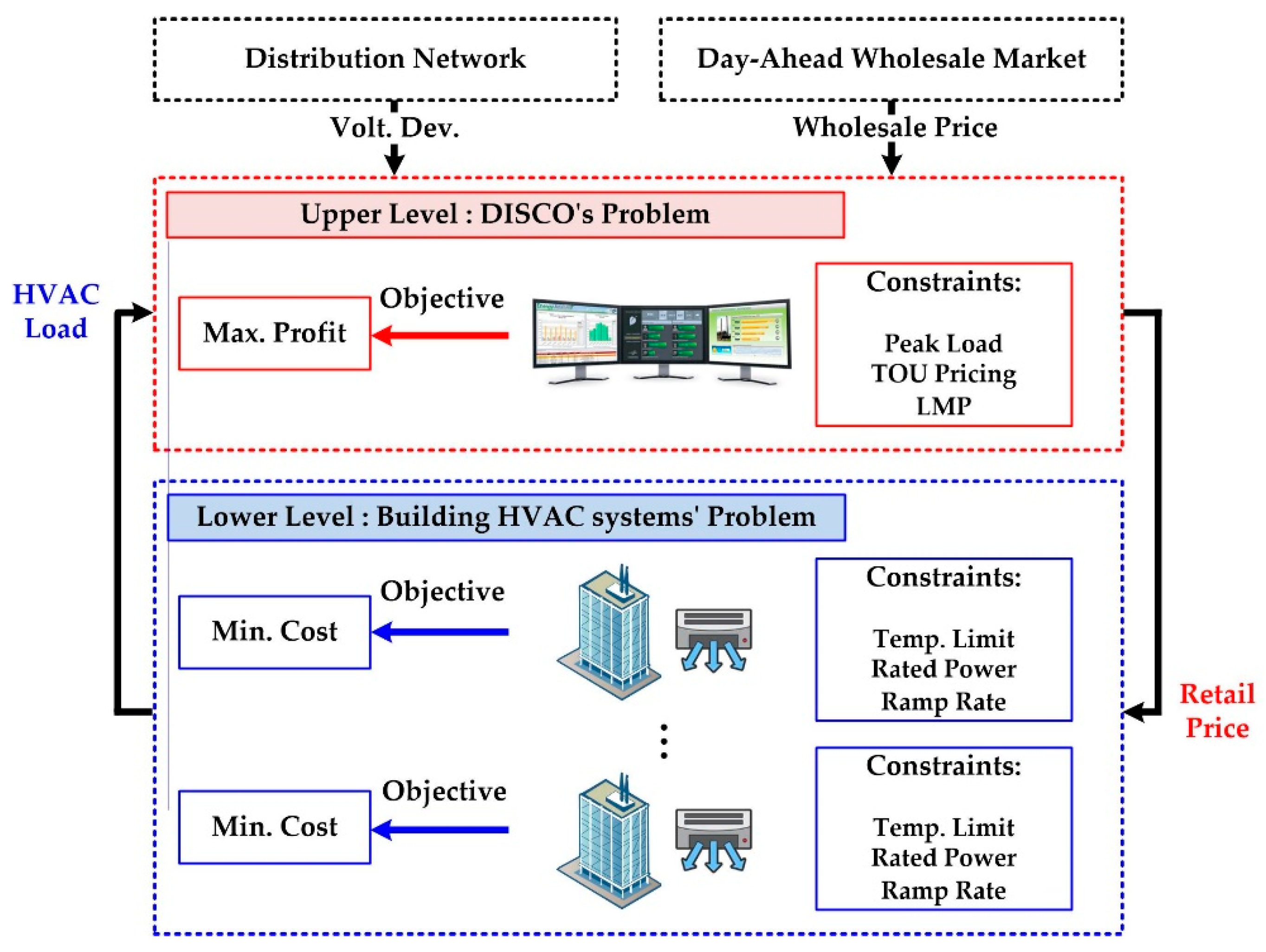
Figure 1 shows the framework of the proposed optimal retail pricing strategy. The EUC buys electricity from the day-ahead wholesale market at LMP and sells it to consumers at two retail prices, namely TOU and real-time pricing (RTP). The LMP represents the price to buy and sell power at different locations within wholesale electricity markets. In this paper, LMP can be considered simply as a wholesale electricity price. The TOU rates typically applies to usage over broad blocks of hours where the electricity price for each period is predetermined and constant. In this paper, we consider the TOU as simply the retail price paid by the end-users. The conventional building operator operates the HVAC systems to maintain a set temperature regardless of the electricity price. The conventional HVAC systems do not participate in the DR service and pay for electricity at the conventional price scheme, TOU (i.e., common price scheme at the distribution level) [24]. However, the proposed retail price on an hourly basis is applied to HVAC systems participating price-based DR service. We have assumed that the end-users are rational to adjust the power inputs of HVAC systems, so that they minimize the electricity bills as long as the thermal comforts are satisfied; i.e., the indoor temperatures are maintained within the acceptable ranges. In addition, smart grid technologies such as advanced metering infrastructures (AMIs) and behind-the-meter energy storage systems have been developing rapidly and continuously during the last decade. Moreover, significant attention has been given to developing energy-efficient devices, homes, or buildings and integrating a large number of renewable energy resources into power grid, to mitigate global warming and climate change. The development of such technologies and applications makes end-users become more aware of the rational use of electricity. For the same reason, the assumption on minimizing the end-users’ electricity bills can be commonly made in many previous studies on price-based DR scheduling [15] and [25,26]. The EUC ensures that the proposed price is always less than the TOU to induce DR participation of HVAC systems in commercial buildings. Therefore, the 24-h operating costs of the price-sensitive HVAC units are cheaper than those of the conventional units. The EUC can effectively attract more HVAC units to its DR program participating the proposed pricing program.

As shown in Figure 1, the EUC determines the optimal profile of the retail price for the scheduling time (i.e., 24 h) to maximize its net profit, which is equivalent to the difference between the total revenue of selling electricity to HVAC systems and the total cost of purchasing electricity from the wholesale market. The EUC seeks to reduce peak loads to bypass costly additional facility (i.e., substations or lines) expansion. Therefore, the EUC changes the retail price to exploit the demand-side flexibility of the price-sensitive HVAC loads for peak load reduction. For the optimal profile of retail price, the building operators schedule the optimal power consumptions of HVAC systems so as to minimize their electricity bills while ensuring the thermal comforts of occupants.

For the proposed framework, a bi-level optimization problem is formulated to reflect the hierarchical decision models of the EUC and the consumers (i.e., leader and followers) in the upper- and lower-decision levels, respectively. In this sense, the proposed pricing framework is related to the Stackelberg games in economics [27]. The optimization problem is transformed to an equivalent single-level problem using the Karush–Kuhn–Tucker (KKT) condition and the penalty method [9]. The EUC solves the single-level problem to maximize its profit, considering that the consumers minimize their electricity bills while satisfying the occupants’ thermal comfort.

In addition, an accurate but simple thermal dynamic model (i.e., an experimental, data-driven model of the actual HVAC system) needs to be developed to estimate the indoor temperature variations for the power input changes of HVAC system, which requires a comprehensive understanding of the thermal dynamics of the target buildings under time-varying indoor and outdoor environmental conditions. We also need to pay careful attention when integrating the thermal dynamic model into the optimization problem, so that common solvers in the off-the-shelf software programs can be readily applied to find the optimal solution within a reasonable computational time. Comprehensive models of building thermal dynamics can be developed using a range of commercial software, for example, TRNSYS, Dymola/Modelica, and EnergyPlus. However, these comprehensive models are often too sophisticated and slow to be applied to the 24-h optimal scheduling problem where the EUC communicates with a number of buildings located throughout the distribution network. To resolve this challenge, the experimental data-driven models of a building room and HVAC system were adopted and integrated into the optimal scheduling problem in the proposed retail pricing strategy.

2.2. Modeling the Thermal Response of HVAC Systems in Commercial Buildings

In this paper, the thermal dynamic response of an HVAC system in a small office building of United States was modeled based on the experimental building room thoroughly described in [13]. As shown in Figure 2, it is divided into a climate room and a test room, both in a larger laboratory room with a constant indoor temperature. The test room includes lights and general heat sources to simulate internal heat gains for a common office room. In [13], the thermal dynamic model of the test room was implemented using a regression-based inverse transfer function to characterize the linear dependencies on the external and internal environmental parameters during the past and current times as

$$T_{ht}={\displaystyle \sum _{k=t-\tau }^{t-1}{a}_{hk}{T}_{hk}}+{\displaystyle \sum _{k=t-\tau }^t\left(s_{hk}{T}_{ak}+d_{hk}{T}_{xk}+f_{hk}{Q}_{hk}+g_{hk}{Q}_{ck}+k_{hk}{Q}_{rk}\right)},\forall h,\forall t$$

(1)

In (1), T_ht is the indoor temperature adjusted by HVAC system h, T_at is the adjacent room temperature, and T_xt is the ambient temperature. In addition, Q_ht is the cooling rate provided by HVAC unit h, and Q_ct and Q_rt are the heat gains from convective and radiative internal loads, respectively. The coefficients a_ht–k_ht depend on building orientation, structure, and materials. The adjacent and ambient temperatures, as well as the internal heat gains, can be measured and forecast using historical data acquired during normal building operation [14]. In this study, we focus on the relations between T_ht and Q_ht by simplifying (1) to (2) where l_ht represents the building environmental parameters. The coefficients a_ht, s_ht, d_ht, f_ht, g_ht, and k_ht in (1) were estimated as shown in

Table 1. Coefficients for the inverse transfer function (ITF) model (1) that were experimentally obtained in [28].

ah(t–3)	ah(t−2)	ah(t−1)	sh(t−3)	sh(t−2)	sh(t−1)	sht
−5.08 × 10−1	6.84 × 10−1	8.13 × 10−1	1.07 × 10−3	1.07 × 10−3	1.07 × 10−3	1.07 × 10−3
dh(t−3)	dh(t−2)	dh(t−1)	dht	fh(t−3)	fh(t−2)	fh(t−1)	fht
−9.31 × 10−3	−1.06 × 10−2	1.34 × 10−2	1.32 × 10−2	1.46 × 10−3	−3.54 × 10−3	−1.25 × 10−3	3.75 × 10−3
gh(t−3)	gh(t−2)	gh(t−1)	ght	kh(t−3)	kh(t−2)	kh(t−1)	kht
1.46 × 10−3	−3.54 × 10−3	−1.25 × 10−3	3.75 × 10−3	4.08× 10−5	−1.24 × 10−3	1.49 × 10−4	1.44× 10−3

. The coefficients were obtained by developing and validating simulation models in [28].

$$T_{ht}={\displaystyle \sum _{k=t-\tau }^{t-1}{a}_{hk}{T}_{hk}}+{\displaystyle \sum _{k=t-\tau }^t(f_{hk}{Q}_{hk}+l_{hk})},\forall h,\forall t$$

(2)

Although the small test building, shown in Figure 2, has been used here for simplicity, the thermal dynamic modeling and, hence, the proposed optimal pricing strategy can be easily applied to large-scale, multi-zone commercial buildings using different thermal coefficients in (1) and (2) [13,29].

The thermal dynamic model is incorporated particularly with the model of a variable speed heat pump (VSHP), which is a common example of an HVAC system. This leads the cooling rate provided by the VSHP unit h at time t to be represented [13] as:

$$Q_{ht}=z_{3,ht}{\left({\displaystyle \sum _{m=1}^{N_L}{\delta }_{mht}}\right)}^3+z_{2,ht}{\left({\displaystyle \sum _{m=1}^{N_L}{\delta }_{mht}}\right)}^2+z_{1,ht}{\displaystyle \sum _{m=1}^{N_L}{\delta }_{mht}}+z_{0,ht},\forall h,\forall t$$

(3)

In (3) and (4), δ_mht is the m_th power segment of the VSHP unit h at time t and z_0,ht–z_3,ht are the coefficients dependent on the steady-state operating conditions (i.e., δ_mht and T_xt) of the VSHP unit h at time t. As discussed in [13], Q_ht is also affected by the mixed-air temperature in the air-handling unit, which in general is maintained at 26 °C. We assumed that the return air temperature is kept the same as the indoor temperature if a supply air lower than 25 °C (i.e., maximum indoor temperature) is introduced into the room. Therefore, the return air temperature is lower than 26 °C. Under these conditions, it is assumed that the return air is mixed with a small amount of outdoor air in order to reduce the loss of cooling energy in buildings and to maintain indoor air quality above a certain level [30]. In [30], the mixed air temperature was set to constant 26 °C, but it showed the same effect even if the mixed air temperature is higher than 26 °C. By combining (2) and (3), the indoor temperature for the input power of the VSHP can be simply expressed as

$$T_{ht}={\displaystyle \sum _{k=1}^t{f}_k({\delta }_{mhk})},\forall h,\forall t$$

(4)

Figure 3 shows an example of the nonlinear curves obtained using (4). In Figure 3, T_z,ht is defined as the indoor temperature at time t for Q_hk = 0 for 0 ≤ k ≤ t; i.e., the HVAC system is turned off during the period. Furthermore, F_mhtj is the linear gradient of T_ht at time t = j for the m_th power segment of HVAC system h at time t = k (i.e., k ≤ j). N_L represents the number of piecewise linear blocks. The nonlinear thermal dynamic response of the building room to the input power variation of HVAC unit can be approximated to (5) using a piecewise linearization approach where the operating range from 0 to P_h,max of HVAC system is divided into N_L segments.

$$T_{ht}\cong T_{z,ht}+{\displaystyle \sum _{m=1}^{N_L}{\displaystyle \sum _{j=1}^t{F}_{mhtj}{\delta }_{mhj}}},\forall h,\forall t$$

(5)

This approach aims to develop a set of linear constraints on the indoor temperature variation, as discussed in Section 3, which can be applied to the KKT conditions. Consequently, the bi-level decision model for the proposed optimal pricing strategy can be converted into the single-level decision model.

3. Optimization Problem Formulation

For the proposed framework discussed in Section 2, the optimal electricity price schedule and corresponding input power profile of HVAC units can be determined by solving the upper-level problem and lower-level problem, respectively.

3.1. Upper-Level Problem

$$\underset{C_t}{\arg \max }{J}_{DP}=N_{HVAC}{\displaystyle \sum _{t=1}^{N_T}(C_t-M_t){\displaystyle \sum _{h=1}^{N_H}{\displaystyle \sum _{m=1}^{N_L}{\delta }_{mht}}}}$$

(6)

$$N_{HVAC}=R_H{\displaystyle \sum _{t=1}^{N_T}{P}_{T,t}}/{\displaystyle \sum _{t=1}^{N_T}{\displaystyle \sum _{h=1}^{N_H}{P}_{C,ht},\forall h,\forall t}}$$

(7)

$$M_t\le C_t\le U_t,\forall t$$

(8)

$$P_{R,t}=P_{T,t}-N_{HVAC}{\displaystyle \sum _{h=1}^{N_H}{P}_{C,ht}},\forall t$$

(9)

$$N_{HVAC}{\displaystyle \sum _{h=1}^{N_H}{\displaystyle \sum _{m=1}^{N_L}{\delta }_{mht}}}+P_{R,t}\le P_{peak},\forall t$$

(10)

The EUC determines the optimal retail price C_t to maximize its profit J_DP by solving the upper-level problem (6)–(10). In (6), the EUC’s profit J_DP is calculated as the difference between the revenue of selling the electricity to the price-sensitive HVAC systems at C_t and the cost of purchasing the electricity at M_t from the wholesale market. N_T is the number of scheduling time intervals in a day. The conventional HVAC systems were assumed to consume pre-determined input power P_C,ht for 5 ≤ t ≤ 19 to maintain the indoor temperature at 22.5 °C during 8 ≤ t ≤ 19. The EUC’s profit J_DC = ∑_t (U_t –M_t) × ∑_h, P_C,ht in business with the conventional HVAC systems is constant, because the TOU price U_t is also determined in advance. It can then be added to (6), resulting in the total profit of the EUC J_D = J_DP + J_DC.

In (7), the ratio of the power consumption of HVAC systems in the commercial buildings to the total power consumption in the distribution network is set to R_H and used to determine the total number of commercial HVAC systems in the distribution network. N_H is the number of the types of HVAC systems and N_HVAC is the total number of HVAC systems in the distribution system divided by N_H.

The EUCs are regulated not to maximize their profit by manipulating the prices; therefore, we set (8) to prevent EUC from setting its price to maximize profit. In addition, (8) represents the upper and lower limits of C_t at time t, which are equivalent to U_t and M_t, respectively. This allows consumers to reduce their electricity bills via the proposed retail pricing scheme, and, consequently, the EUC can attract a number of HVAC loads to its optimal price-based DR strategy, procuring substantial load flexibility. The constraints (8) can also reduce the exposure consumers have to highly volatile prices and alleviate the EUC’s market power by preventing the EUC from increasing its profit excessively, which appears to be unfair to consumers. It was assumed in [31] that the EUC and consumers reach such an agreement to bring (8) into effect.

In (9), P_R,t is defined as the remainder load other than the load used in conventional HVAC systems. N_HVAC ·∑_h ∑_m δ_mht + P_R,t is established to estimate the peak limit P_peak because of price-sensitive HVAC loads in (10).

3.2. Lower-Level Problem

$$\underset{{\delta }_{mht}^{}}{\arg \min }{J}_{BP}^{}={\displaystyle \sum _{t=1}^{N_T}{C}_t{\displaystyle \sum _{h=1}^{N_H^{}}{\displaystyle \sum _{m=1}^{N_L}{\delta }_{mht}^{}}}}$$

(11)

$${\delta }_{mh,\max }^{}\cdot b_{mht}^{}\le {\delta }_{mht}^{}\le {\delta }_{mh,\max }^{},\mathrm{for}m=1,\forall h,\forall t$$

(12)

$${\delta }_{mh,\max }^{}\cdot b_{mht}^{}\le {\delta }_{mht}^{}\le {\delta }_{mh,\max }^{}\cdot b_{(m-1)ht}^{},\mathrm{for}2\le m\le N_L-1,\forall h,\forall t$$

(13)

$$0\le {\delta }_{mht}^{}\le {\delta }_{mh,\max }^{}\cdot b_{(m-1)ht}^{},\mathrm{for}m=N_L,\forall h,\forall t$$

(14)

$$0\le {\displaystyle \sum _{m=1}^{N_L}{\delta }_{mht}^{}}\le P_{h,\max }^{},\forall h,\forall t$$

(15)

$$D_L^{}\le \left({\displaystyle \sum _{m=1}^{N_L}{\delta }_{mht}}-{\displaystyle \sum _{m=1}^{N_L}{\delta }_{mh(t-\Delta {\mathrm{t}}_{unit})}}\right)/\Delta {\mathrm{t}}_{unit}\le D_U,\forall h,\forall t$$

(16)

$$T_{ht,\min }^{}\le T_{z,ht}^{}+{\displaystyle \sum _{m=1}^{N_L}{\displaystyle \sum _{j=1}^t{F}_{mhtj}^{}\cdot {\delta }_{mhj}^{}}}\le T_{ht,\max }^{},\forall h,\forall t$$

(17)

For the price-sensitive HVAC units, the optimal power inputs ∑_m δ_mht for all h are scheduled to minimize their operating cost J_BP, given C_t, by solving the lower-level problem (11)–(17). The operations of the conventional HVAC units result in the constant operating cost J_BC = ∑_tU_t × ∑_h P_C,ht, which can be simply added to (11) as J_B = J_BP + J_BC without affecting the optimal schedules of δ_mht. To complete the piecewise linear approximation, (12)–(14) are established to describe the boundary conditions on δ_mht, as shown in Figure 3, using the binary variables b_mht. For example, for b_2ht = 1, b_3ht = 0, and b_4ht = 0, δ_3ht can be scheduled to the value between 0 and δ_3h,max, whereas δ_4ht is forced to be zero. Moreover, (15) specifies that the scheduled power inputs ∑_m δ_mht of HVAC systems need to be less than their rated power P_h,max, and (16) specifies the limits D_L and D_U on the positive and negative ramp rates of ∑_m δ_mht, respectively, during the unit time interval ∆t_unit = 1 h. In general, D_U needs to be carefully determined by considering practical operation of heat pumps (HPs) to prevent severe operational stress on HP compressors. Furthermore, the inequality constraints (17) specify that the indoor temperature T_ht should be maintained within an acceptable range between T_ht,min and T_ht,max so as to satisfy the occupants’ thermal comfort. Note that T_ht is approximated using a piecewise linear equation (5) for the application of the KKT conditions.

3.3. Equivalent Single-Level Problem

$${\nabla }_{{\delta }_{mht}}L(C_t,{\delta }_{mht},{\eta }_{\lambda mht},{\beta }_{\rho mht},{\alpha }_{\psi ht},{\mu }_{\omega ht})=0,\forall m,\forall h,\forall t,\forall \lambda ,\forall \rho ,\forall \psi ,\forall \omega$$

(18)

$$0\le d_{\lambda }({\delta }_{mht},b_{mht})\perp {\eta }_{\lambda mht}\ge 0,\forall m,\forall h,\forall t,\forall \lambda$$

(19)

$$0\le h_{\rho }({\delta }_{mht})\perp {\beta }_{\rho mht}\ge 0,\forall m,\forall h,\forall t,\forall \rho$$

(20)

$$0\le g_{\psi }({\delta }_{mht})\perp {\alpha }_{\psi ht}\ge 0,\forall m,\forall h,\forall t,\forall \psi$$

(21)

$$0\le y_{\omega }(T_{ht})\perp {\mu }_{\omega ht}\ge 0,\forall h,\forall t,\forall \omega$$

(22)

We apply the KKT conditions to the lower level problem. The binary variables b_mht in (12)–(14) were relaxed to real variables as 0 ≤ b_mht ≤ 1 without changing the optimal input power schedules of δ_mht. In other words, the linear programming relaxation turns out to be exact [32], because the slopes of the piecewise linearized curves in Figure 3 are monotonously reduced, as HVAC load is increased. For the temperature control, it is still cost-effective to increase the input power of HVAC system gradually from ∑_m δ_mht = 0 to the rated value ∑_m δ_mht = P_h,max. Using the KKT conditions, (11)–(17) can be equivalently replaced with (18)–(22). η_λmht, β_ρmht, α_ψht, and μ_ωht are Lagrangian multipliers.

The original bi-level problem can then be reformulated with the single-level objective function (23):

$$\underset{C_t,{\delta }_{mht}}{\arg \max }{J}_{DP}={\displaystyle \sum _{t=1}^{N_T}{C}_t{\displaystyle \sum _{h=1}^{N_H^{}}{\displaystyle \sum _{m=1}^{N_L}{\delta }_{mht}^{}}}}-J\left({\delta }_{mht}^{},M_t\right)$$

(23)

Owing to the non-linearity of the first term in (23) and the complementarity of (19)–(22), an interior-point solver in conjunction with a penalty method has been applied, as discussed in [33], by converting (19)–(22) to (25) where Θ is the upper bound of the total sum. The equivalent single-level problem can then be expressed as

$$\underset{C_t,{\delta }_{mht}}{\arg \max }{J}_{DP}=N_{HVAC}{\displaystyle \sum _{t=1}^{N_T}{C}_t{\displaystyle \sum _{h=1}^{N_H^{}}{\displaystyle \sum _{m=1}^{N_L}{\delta }_{mht}^{}}}}-N_{HVAC}{\displaystyle \sum _{t=1}^{N_T}{M}_t{\displaystyle \sum _{h=1}^{N_H^{}}{\displaystyle \sum _{m=1}^{N_L}{\delta }_{mht}^{}}}-}\pi \cdot \mathsf{\Theta }$$

(24)

Subject to (7)–(10) and (12)–(18)

$$\begin{array}{l}{\displaystyle \sum _{\lambda =1}^{N_{\lambda }}{\displaystyle \sum _{h=1}^{N_H}{\displaystyle \sum _{t=1}^{N_T}{\displaystyle \sum _{m=1}^{N_L}{\eta }_{\lambda mht}\cdot d_{\lambda }({\delta }_{mht},b_{mht})}}}}+{\displaystyle \sum _{\rho =1}^{N_{\rho }}{\displaystyle \sum _{h=1}^{N_H}{\displaystyle \sum _{t=1}^{N_T}{\displaystyle \sum _{m=1}^{N_L}{\beta }_{\rho mht}\cdot h_{\rho }({\delta }_{mht})}}}}\\ \hspace{1em}\hspace{1em}\hspace{1em}\hspace{1em}\hspace{1em}+{\displaystyle \sum _{\psi =1}^{N_{\psi }}{\displaystyle \sum _{h=1}^{N_H}{\displaystyle \sum _{t=1}^{N_T}{\displaystyle \sum _{m=1}^{N_L}{\alpha }_{\psi ht}\cdot g_{\psi }({\delta }_{mht})}}}}+{\displaystyle \sum _{\omega =1}^{N_{\omega }}{\displaystyle \sum _{h=1}^{N_H}{\displaystyle \sum _{t=1}^{N_T}{\mu }_{\omega ht}\cdot y_{\omega }(T_{ht})}}}\le \mathsf{\Theta }\end{array}$$

(25)

$${\mu }_{\omega ht}\ge 0,{\alpha }_{\psi ht}\ge 0,{\beta }_{\rho mht}\ge 0,{\eta }_{\lambda mht}\ge 0,\forall m,\forall h,\forall t,\forall \omega ,\forall \psi ,\forall \rho ,\forall \lambda$$

(26)

In (24), π is defined as the penalty factor. For a positive constant π, Θ becomes zero when (19)–(22) are satisfied [9,33].

4. Simulation Case Studies and Results

4.1. Test System and Simulation Conditions

In the case studies, the effect of the proposed pricing strategy on the peak load reduction are explicitly investigated for the cases of conventional load demand and duck curve, and the data in Figure 4b–d are from United States (i.e., test site). A 24-h load demand curve during summertime was adopted from [34] and scaled down, so that the distribution network has the peak load demand of 7.04 MW at t = 17 h, as shown by the blue line in Figure 4a. The PV production time-series (i.e., red line in Figure 4a) was acquired from [35] and scaled up to 20% of the peak of the conventional load curve (i.e., the blue line in Figure 4a). The load curve that changed with the introduction of PV is represented by the green line shown in Figure 4a. The peak load of the green line is 6.61 MW at t = 20 h. The 24-h curve of the ambient air temperature [36], shown in Figure 4b, is similar to the conventional load demand curve. In particular, both the maximum temperature and the peak load took place at t = 17 h. In addition, Figure 4c indicates the curves of the wholesale price M_t [37] and retail price U_t for the TOU scheme [38]. It was assumed that the EUC was informed of M_t one day ahead to schedule the optimal C_t considering the price-based DR of HVAC units. For the optimal C_t, the input power of HVAC systems was then determined, given the N_H profiles of the building thermal loads, which were developed as shown in Figure 4d based on the real data in [30] and [39]. Specifically, the VSHP load profiles in a real commercial building were measured and then scaled down with the different ratios to determine the rated power inputs of the VSHPs. For the rated inputs, the corresponding cooling rates Q_ht were then estimated using (3), and the scaled fractions of Q_ht were applied to the control of T_ht. As shown in Figure 4d, the N_H type profiles of thermal energy loads Q_ct and Q_rt were then determined for the test buildings. In this paper, we assumed that the internal heat gain could be forecasted as Figure 4d. Based on the real profiles of ∑_m δ_mht, Q_ht, and T_xt, for simplicity, it was assumed that the group of buildings has the same thermal load profile. Figure 4d shows that the thermal loads were increased at t = 7 h (when people started coming to work) and were maintained at high levels until t = 19 h, when the workers left the buildings.

Table 2. Power capacity and cooling rate of the HVAC systems and maximum heat gain per building room.

No	Ph,max [kW]	Qh,max [kW]	(Qc + Qr)max [W]	No	Ph,max [kW]	Qh,max [kW]	(Qc + Qr)max [W]
1	26	118	708	9	27	123	727
2	24	109	725	10	29	132	639
3	26	118	675	11	25	114	653
4	24	109	698	12	19	86	709
5	21	95	721	13	22	100	721
6	19	86	723	14	20	91	717
7	23	105	704	15	24	109	701
8	21	95	713

lists the rated values of ∑_m δ_mht and Q_ht of HVAC units and maximum value of (Q_ct + Q_rt) per building room.

As mentioned in Section 3, N_H types of HVAC systems were used and the total number of HVAC systems included in the distribution network was N_H × N_HVAC. In this paper, N_H was set to 15 as shown in Table 2. As mentioned in Section 1, more than 13% of the total energy usage is consumed by commercial HVAC systems, so the case studies were simulated with R_H = 0.13. In the case of the conventional load profiles, N_HVAC is set to 6 by (7), and in the case of duck curve, N_HVAC is set to 4.6 by (7).

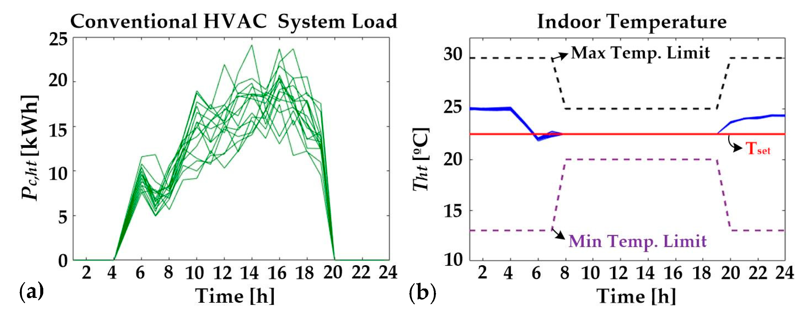
Figure 5a shows that the input power of the conventional HVAC systems varied over the scheduling time period to maintain T_ht at T_set = 22.5 °C during the working hours (i.e., 8 h ≤ t ≤ 19 h), as shown in Figure 5b, given the time-varying thermal conditions T_xt, Q_ct, and Q_rt of the buildings. It was assumed that the conventional HVAC systems are operated during 5 h ≤ t ≤ 19 h.

In addition, the load factor and load leveling index are introduced to analyze the effect of the proposed pricing strategy on the peak load reduction. In [40], the load factor can be defined as the ratio of the average demand to the peak load as:

$$loadfactor=\frac{{\displaystyle \sum _{t=1}^{N_T}{P}_t}/N_T}{\underset{t\in N_{time}}{\max }{P}_t}$$

(27)

The load leveling index is the MSE with respect to the reference value as [41]:

$$MS{E}_{loadleveling}=\frac{1}{N_T}{\displaystyle \sum _{t=1}^{N_T}(P_t-}{\displaystyle \sum _{t=1}^{N_T}{P}_t/N_T{)}^2}$$

(28)

4.2. Case Study A: Two Types of Load Profiles

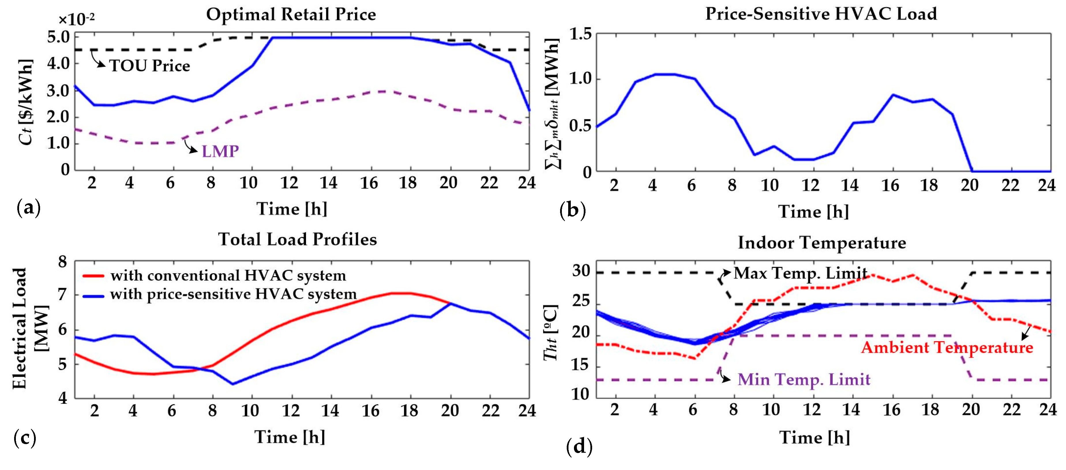
Figure 6a shows the optimal schedules of C_t for the proposed pricing strategy considering peak load reduction applied to conventional load curve, and Figure 6b,d show the corresponding data on the total power inputs of the price-elastic HVAC units and the indoor temperatures in the building rooms. In Figure 6c, the red line shows the total load curve when HVAC systems are operated in the conventional manner, and the blue line shows the total load curve when HVAC systems are operated by the price sensitive method.

In Figure 6a, the EUC maintained C_t as sufficiently low in the early morning (i.e., 1 h ≤ t ≤ 8 h), taking into account that the end-users aim to minimize the operating cost of their HVAC systems. This led to the pre-cooling of HVAC systems, reducing the indoor temperature before people come to work. Specifically, the large input power of the HVAC systems was scheduled during the time period of 3 h ≤ t ≤ 7 h, even though the ambient temperature and thermal energy loads were maintained high during 8 h ≤ t ≤ 19 h. Owing to the low retail price in the early morning, HVAC loads were shifted away from on-peak hours to off-peak hours (i.e., early morning), leading to the pre-cooling operation and a reduction in the EUC’s profit and building operators’ operation cost. In Figure 6d, the pre-cooled indoor temperature increased gradually from 20 °C at t = 8 h to 25 °C at t = 12 h, as the ambient temperature and internal heat gains increased. Because of the limited thermal capacity in the building structures, HVAC loads started increasing at t = 13 h for satisfying occupants’ comforts (i.e., temperature constraints). During 11 h ≤ t ≤ 19 h, the EUC sets C_t to the upper limit to compensate for the reduction in the EUC’s profit, resulting from the low value of C_t for the pre-cooling. Specially, the EUC sets C_t to the upper limit to lower power consumption during on-peak hours (i.e., 16 h ≤ t ≤ 19 h). To prevent excessive compensation of the EUC’s profit, the upper limit was set as the TOU price U_t, as shown in (8), mitigating the retail price volatility and ensuring the financial benefit of the consumers participating in the proposed pricing scheme. In Figure 6c, the peak load of the total load containing the conventional HVAC system is 7.04 MW, while the peak load of the total load containing the proposed price-sensitive HVAC system is 6.75 MW and the reduction rate is approximately 4.18%. In the proposed method, the peak of the total load curve takes place at t = 20 h. The peak load reduction rate cannot be increased further because HVAC system does not need to operate for 20 h ≤ t ≤ 24 h owing to the mitigation of the indoor temperature constraints. However, the difference between the peak and minimum load values shows that the proposed method does not improve in terms of load leveling with 2.33 MW for the conventional HVAC system and 2.32 MW for the price-sensitive HVAC system.

Table 3. Reductions of the operating costs (J_BP,h and J_BC,h) for individual HVAC units.

HVAC unit	1	2	3	4	5	6	7	8	9	10	11	12	13	14	15
(1) JBP,h [$]	4.85	4.92	4.15	4.75	5.30	4.58	4.28	4.44	4.70	4.61	3.52	4.35	5.26	3.59	3.81
(2) JBC,h [$]	10.72	11.11	9.14	10.38	11.74	10.33	9.42	10.00	10.41	10.22	7.99	9.51	11.80	7.94	8.36
((2)-(1))/(2) [%]	54.78	55.67	54.62	54.24	54.88	55.67	54.58	55.54	54.80	54.91	55.96	54.29	55.42	54.79	54.48

summarizes the J_BP and J_BC for individual HVAC units for the proposed pricing scheme and the TOU pricing scheme, respectively, for peak load reduction of the conventional load curve. The 24-h operating costs J_BP of the price-sensitive HVAC units are cheaper than those of the conventional units. This demonstrates that using the proposed pricing scheme, the EUC can effectively attract more HVAC units to its DR program.

As shown in Figure 7, the optimal schedules of C_t and ∑_m δ_mht were determined by proposed pricing strategy considering peak load reduction applied to duck curve. The peak load of the duck curve occurs at t = 20 h, as shown in Figure 7c. The commercial HVAC system does not need to be operated for 20 h ≤ t ≤ 24 h owing to mitigation of the indoor temperature conditions. As a result, the commercial HVAC system cannot affect the load curve after 20 h. In the proposed method (i.e., blue line) in Figure 7c, the difference between the peak load and the minimum value of the load curve is larger than the conventional strategy (i.e., red line). In other words, even if the EUC utilizes the commercial HVAC system as a DR resource, the peak load of duck curve cannot be reduced.

4.3. Case Study B: Purpose of Demand Response

We demonstrated that the proposed pricing strategy could be applied to other purpose such as load leveling besides peak load reduction. The simple constraint (i.e., P_min < N_HVAC·∑_m δ_mht + P_R,t) was added to (10) to show that price-sensitive HVAC systems can have positive effects even in terms of load leveling, and, the simulation results of applying the proposed pricing strategy to the conventional load curve are shown in Figure 8. To satisfy the added constraint, the EUC lowered C_t for 6 h ≤ t ≤ 13 h to induce the power consumption of HVAC system. In particular, the blue line in Figure 8a had a minimum value at t = 6 h, and the EUC set C_t close to the lower limit to increase power consumption during this time period. For HVAC system, the input power of the previous time zone affects the indoor temperature of the subsequent time zone, as shown in (4). Therefore, an increase in power consumption for 6 h ≤ t ≤ 8 h could violate the indoor temperature conditions at t = 8 h; this problem could be solved by increasing C_t for 1 h ≤ t ≤ 3 h to reduce the power consumption for 1 h ≤ t ≤ 3 h. The difference between the peak load and minimum values is 1.51 MW, a significant reduction from 2.33 MW for conventional HVAC systems.

Figure 9 shows the simulation results of applying the proposed pricing strategy considering load leveling to the duck curve. The blue line in Figure 9c shows that the difference between the peak load and the minimum load is similar to that of the conventional method (i.e., red line); however, the blue line also shows a more rapid change in power consumption for 16 h ≤ t ≤ 20 h. In other words, the total load profile (i.e., blue line) of the price-sensitive HVAC systems requires larger ramp rate of generators for 16 h ≤ t ≤ 20 h. As a result, even if the EUC utilizes the commercial HVAC system as a DR resource, the duck curve cannot be improved in terms of load leveling, as shown in Figure 9c.

Figure 9 shows the simulation results of applying the proposed pricing strategy considering the load leveling to the duck curve. The blue line in Figure 9c shows that the difference between the peak load and the minimum load is similar to that of the conventional method (i.e., red line); however, the blue line also shows a more rapid change in power consumption for 16 h ≤ t ≤ 20 h. In other words, the total load profile (i.e., blue line) of the price-sensitive HVAC systems requires larger ramp rate of generators for 16 h ≤ t ≤ 20 h. As a result, even if the EUC utilizes the commercial HVAC system as a DR resource, the duck curve cannot be improved in terms of load leveling, as shown in Figure 9c.

4.4. Case Study C: Parameter Sensitivity

In Section 4.4, we performed the simulation with several value of TOU pricing to demonstrate the applicability of the proposed pricing strategy, because the TOU pricing varies depending on the country or month. Figure 10 shows the effect of the price cap U_t on the optimal profile of the C_t. Figure 10a,b show that as U_t ^max increased, C_t increased accordingly; however, the overall profiles of C_t and, consequently, the overall profiles of the EUC’s profit remained similar. Note that in Figure 10c, the difference value between U_t ^max and U_t ^min were maintained at the same values. Figure 10b,d show the optimal profiles of C_t for the different profiles of U_t shown in Figure 10a,c, respectively. The C_t profiles, apart from the magnitudes, look similar for all cases particularly during the time period from 1 h to 19 h; note that HVAC systems were turned off in the period 20 h ≤ t ≤ 24 h because of low occupancy.

4.5. Discussion

The results for various case studies are summarized in

Table 4. Comparison of the data obtained applying the proposed method and conventional method to the conventional load curve.

	Case A: Conventional Load Curve			Reduction Rate
	(a) Conventional	(b) Peak Reduction	(c) Load Leveling	[(a)–(b)]/[a]	[(a)–(c)]/[a]
peak [MW]	7.04	6.75	6.75	4.12%	4.12%
peak–min. [MW]	2.33	2.32	1.51	0.43%	35.19%
load factor	0.8396	0.8341	0.8388	0.66%	0.10%
MSE load leveling [%]	6911.12	4175.25	2571.28	39.59%	62.80%
JDP [$]	457.21	198.82	149.14	56.51%	67.38%
total profit [$]	3795.47	3537.08	3493.97	6.81%	7.94%

and

Table 5. Comparison of the data obtained applying the proposed method and conventional method to the duck curve.

	Case B: Duck Curve			Reduction Rate
	(a) Conventional	(b) Peak Reduction	(c) Load Leveling	[(a)–(b)]/[a]	[(a)–(c)]/[a]
peak [MW]	6.61	6.61	6.61	0%	0%
peak-min. [MW]	1.89	2.25	1.94	−19.05%	−2.65%
load factor	0.8358	0.8029	0.8012	3.94%	4.14%
MSE load leveling [%]	3753.35	4877.88	4208.09	−29.96%	−12.12%
JDP [$]	350.53	159.45	109.58	54.51%	68.74%
total profit [$]	3580.88	3389.79	3339.93	5.34%	6.73%

. In Table 4, the proposed method reduced the peak load of the conventional load curve by 4.12% compared to the conventional method. In terms of load leveling, the proposed method, which only considers the peak load reduction, reduced the difference between the peak load and the minimum load by 0.43% compared to the conventional method, and reduced by 35.19% when the constraint for the load leveling is added. The load factor has similar values in the cases of (a)–(c). The proposed method did not improve the load curve in terms of load factor. However, the proposed method reduced the load leveling index by 39.59% in the case of (b) and 62.80% in the case of (c), compared to the conventional method. The load leveling index is further reduced in the case of (c) where load leveling constraints are added compared to the case of (b) with only constraints of peak load reduction. The proposed method effectively achieved peak load reduction and load leveling. These allow for the postponement of investments in grid upgrades or in new substation capacity. The EUC’s profit for commercial HVAC systems (i.e., J_DP) with the constraint for the peak load reduction is 56.51% less than that of the conventional method. The J_DP is reduced by 67.38% with the addition of load leveling constraint. In other words, by load leveling and reducing the peak load, the profit for commercial HVAC systems is greatly reduced. While the J_DP is greatly reduced, the total profit of the distribution network decreased by 6.81% (peak load reduction) and 7.94% (load leveling), respectively. Although this may initially limit the profit of the EUC, the reduction in profit can be sufficiently compensated for by the savings in the network operating costs that result from the improved load flexibility, e.g., a decrease in the installation costs of new substations and lines.

Table 5 reveals the proposed method did not reduce the peak load of the duck curve. The proposed method for peak load reduction increases the difference between peak and minimum value by −19.05%. Applying the constraint for the load leveling increases the difference between the peak and minimum value by −2.65%. The proposed strategy reduced the load factor in the cases (b) and (c), and has an adverse effect on the load curve in terms of load factor. In addition, the proposed method increased the load leveling index by −29.96% in the case of (b) and −12.12% in the case of (c), compared to the conventional method. However, in the proposed method, the retail price is lower than the TOU price in the conventional method, which reduces the J_DP. As a result, the peak load reduction or load leveling of the duck curve cannot be achieved by using the DR of the commercial HVAC systems. This will be addressed in future studies by inducing DR participation of DR resources such as HVAC systems in residential buildings.

5. Conclusions

This paper proposed an optimal retail pricing scheme to support the EUC and building operators in determining the day-ahead optimal retail price and the corresponding input power of price-elastic HVAC units, respectively, reducing the peak load in the distribution network. A bi-level decision model was adopted to develop the proposed scheme, i.e., in the upper level, the EUC determines the optimal price to maximize its profit and in the lower level, the building operators schedule the optimal input power of HVAC units to minimize their operating costs. The proposed bi-level optimal pricing model was applied to two types of load curves using the experimental data-driven model of an HVAC system in commercial buildings. The optimal retail price was determined to reduce peak load demand, avoiding the cost for reinforcing power equipment and distribution lines. The upper bound of the retail price was set using the TOU pricing rates to achieve the low price volatility in the DR program. The nonlinear thermal dynamic response of an experimental building room to the input power of the VSHP was modeled using a set of piecewise linear equations, which enabled the application of the KKT conditions and the transformation of the bi-level decision model to the single-level model. The results of the case studies demonstrated the effectiveness of the proposed strategy with the following main features:

• The EUC induced the pre-cooling of HVAC systems, considering that the consumers minimize the operating cost of HVAC units. To compensate for the reduction of the EUC’s profit because of the pre-cooling, the EUC determined high retail price during on-peak times. In addition, the building operators scheduled small input power of HVAC system during the on-peak hours to minimize the electricity bills.
• For the conventional load curve, the peak load could be successfully reduced using the pre-cooling of HVAC units. The corresponding reduction of the EUC’s profit can be justified by the opportunity cost of installing an additional line or substation and the reduction in consumers’ electricity bills.
• For the duck curve, as participation in DR of the commercial HVAC systems does not result in peak load reduction or load leveling, residential HVAC systems will also need to be addressed by inducing participation in DR. In addition, we will research additional case studies on the application of the proposed pricing strategy to large-scale, multi-zone buildings.

References

- Strrbac, G.; Gan, C.K.; Aunedi, M. Benefits of advanced smart metering for demand response based control of distribution networks. Rep. Energy Netw. Assoc. UK 2010, 2, 1–46. [Google Scholar]
- Wilks, M. Demand Side Response: Conflict between Supply and Network Driven Optimisation. A Report to DECC; POYRY: Vantaa, Finland, 2010. [Google Scholar]
- Hou, Q.; Zhang, N.; Du, E. Probabilistic duck curve in high PV penetration power system: Concept, modeling, and empirical analysis in China. Appl. Energy 2019, 242, 205–215. [Google Scholar] [CrossRef]
- Rowe, M.; Yunusov, T.; Haben, S. A Peak Reduction Scheduling Algorithm for Storage Devices on the Low Voltage Network. IEEE Trans. Smart Grid 2014, 5, 2115–2124. [Google Scholar] [CrossRef]
- Qdr, Q. Benefits of Demand Response in Electricity Markets and Recommendations for Achieving Them; Technical Report; US Department of Energy: Washington, DC, USA, 2006.
- Hassan, N.U.; Khalid, Y.I.; Yuen, C. Customer engagement plans for peak load reduction in residential smart grids. IEEE Trans. Smart Grid 2015, 6, 3029–3041. [Google Scholar] [CrossRef] [Green Version]
- Yoon, J.H.; Baldick, R. Dynamic Demand Response Controller Based on Real-time Retail Price for Residential Buildings. IEEE Trans. Smart Grid 2014, 5, 121–129. [Google Scholar] [CrossRef]
- Perez, K.X.; Baldea, M.; Edgar, T.F. Integrated HVAC management and optimal scheduling of smart appliances for community peak load reduction. Energy Build. 2016, 123, 34–40. [Google Scholar] [CrossRef] [Green Version]
- Jeong, M.G.; Moon, S.I.; Hwang, P.I. Indirect load control for energy storage systems using incentive pricing under time-of-use tariff. Energies 2016, 9, 558. [Google Scholar] [CrossRef] [Green Version]
- Doostizadeh, M.; Ghasemi, H. A day-ahead electricity pricing model based on smart metering and demand-side management. Energy 2012, 46, 221–230. [Google Scholar] [CrossRef]
- US Energy Information Administration. Annual Energy Outlook 2016 (DOE/EIA-0383). Available online: www.eia.gov/outlooks/aeo/pdf/0383(2016).pdf (accessed on 7 November 2019).
- Kim, Y.J.; Wang, J. Power Hardware-in-the-Loop Simulation Study on Frequency Regulation through Direct Load Control of Thermal and Electrical Energy Storage Resources. IEEE Trans. Smart Grid 2018, 9, 2786–2796. [Google Scholar] [CrossRef]
- Kim, Y.; Norford, L.K. Optimal use of thermal energy storage resources in commercial buildings through price-based demand response considering distribution network operation. Appl. Energy 2017, 193, 308–324. [Google Scholar] [CrossRef]
- Vasudevan, J.; Swarup, K.S. Price based demand response strategy considering load priorities. In Proceedings of the IEEE 6th International Conference on Power Systems (ICPS), New Delhi, India, 4–6 March 2016; pp. 1–6. [Google Scholar]
- Chen, Z.; Wu, L.; Fu, Y. Real-time Price-based Demand Response Management for Residential Appliances via Stochastic Optimization and Robust Optimization. IEEE Trans. Smart Grid 2012, 3, 1822–1831. [Google Scholar] [CrossRef]
- Hanif, S.; Gooi, H.B.; Massier, T. Distributed Congestion Management of Distribution Grids under Robust Flexible Buildings Operations. IEEE Trans. Power Syst. 2017, 32, 4600–4613. [Google Scholar] [CrossRef]
- Huang, S.; Wu, Q.; Oren, S.S. Distribution Locational Marginal Pricing through Quadratic Programming for Congestion Management in Distribution Networks. IEEE Trans. Power Syst. 2015, 30, 2170–2178. [Google Scholar] [CrossRef] [Green Version]
- Zhang, C.; Wang, Q.; Wang, J. Real-time Trading Strategies of Proactive DISCO with Heterogeneous DG Owners. IEEE Trans. Smart Grid 2018, 9, 1688–1697. [Google Scholar]
- Nguyen, D.T.; Nguyen, H.T.; Le, L.B. Dynamic Pricing Design for Demand Response Integration in Power Distribution Networks. IEEE Trans. Power Syst. 2016, 31, 3457–3472. [Google Scholar] [CrossRef]
- Zhang, C.; Wang, Q.; Wang, J. Real-time Procurement Strategies of a Proactive Distribution Company with Aggregator-Based Demand Response. IEEE Trans. Smart Grid 2018, 9, 766–776. [Google Scholar] [CrossRef] [Green Version]
- Zhang, C.; Wang, Q.; Wang, J. Strategy-making for a proactive distribution company in the real-time market with demand response. Appl. Energy 2016, 181, 540–548. [Google Scholar] [CrossRef] [Green Version]
- Heydt, G.T.; Chowdhury, B.H.; Crow, M.L. Pricing and Control in the Next Generation Power Distribution System. IEEE Trans. Smart Grid 2012, 3, 907–914. [Google Scholar] [CrossRef]
- Yuan, Z.; Hesamzadeh, M.R. Implementing Zonal Pricing in Distribution Network: The Concept of Pricing Equivalence. In Proceedings of the IEEE Power Energy Society General Meeting (PESGM), Boston, MA, USA, 17–21 July 2016; pp. 1–5. [Google Scholar]
- Hu, Z.; Kim, J.; Wang, J. Review of dynamic pricing programs in the U.S. and Europe: Status quo and policy recommendations. Renew. Sustain. Energy Rev. 2015, 42, 743–751. [Google Scholar] [CrossRef]
- Liu, W.; Wu, Q.; Wen, F. Day-ahead congestion management in distribution systems through household demand respond and distribution congestion prices. IEEE Trans. Smart Grid 2014, 5, 2739–2747. [Google Scholar] [CrossRef] [Green Version]
- Dehghanpour, K.; Nehrir, M.H.; Sheppard, J.W. Agent-based modeling of retail electrical energy markets with demand response. IEEE Trans. Smart Grid 2018, 9, 3465–3475. [Google Scholar] [CrossRef] [Green Version]
- Lasaulce, S.; Tembine, H. Game Theory and Learning for Wireless Networks; Academic Press: Waltham, MA, USA, 2011; pp. 69–71. [Google Scholar]
- Zakula, T. Model Predictive Control for Energy Efficient Cooling and Dehumidification. Ph.D. Thesis, Massachusetts Institute of Technology, Cambridge, MA, USA, June 2013. [Google Scholar]
- Gayeski, N.; Gange, J.; Armstrong, P. Development of a Low-Lift Chiller Controller and Simplified Precooling Control Algorithm: Final Report; U.S. Department of Energy: Washington, DC, USA, 2011.
- Kim, Y.; Norford, L.K.; Kirtley, J.L. Modeling and analysis of a variable speed heat pump for frequency regulation through direct load control. IEEE Trans. Power Syst. 2015, 30, 397–408. [Google Scholar] [CrossRef]
- Wei, W.; Feng, L.; Shengwei, M. Energy pricing and dispatch for smart grid retailers under demand response and market price uncertainty. IEEE Trans. Smart Grid 2015, 6, 1364–1374. [Google Scholar] [CrossRef]
- Boyd, S.; Vandenberghe, L. Convex Optimization; Cambridge University Press: Cambridge, UK, 2004; pp. 561–562. [Google Scholar]
- Benson, H.Y.; Sen, A.; Shannon, D.F. Interior-point algorithms, penalty methods and equilibrium problems. Comput. Optim. Appl. 2006, 34, 155–182. [Google Scholar] [CrossRef] [Green Version]
- Sharma, D.D.; Singh, S.N. Electrical load profile analysis and peak load assessment using clustering technique. In Proceedings of the IEEE Power Energy Society General Meeting (PESGM), National Harbor, MD, USA, 27–31 July 2014; pp. 1–5. [Google Scholar]
- Tsikalakis, A.G.; Hatziargyriou, N.D. Centralized control for optimizing microgrids operation. IEEE Trans. Energy Convers. 2008, 23, 241–248. [Google Scholar] [CrossRef]
- Weather History for Cambridge. Available online: http://www.wunderground.com/weatherstation/WXDailyHistory.asp?ID=KMACAMBR4&month=7&day=21&year=2012 (accessed on 7 November 2019).
- Day Ahead Market Zonal LBMP; NYISO. Available online: http://www.nyiso.com/public/markets_operations/market_data/maps/index.jsp?load=DAM (accessed on 7 November 2019).
- RATES & TARIFFS; Eversource. Available online: http://www.eversource.com/Content/emac/residential/my-account/billing-payment/rates-tariffs (accessed on 7 November 2019).
- Zakula, T.; Armstrong, P.; Norford, L.K. Modeling environment for model predictive control of buildings. Energy Build. 2014, 85, 549–559. [Google Scholar] [CrossRef]
- Chiu, W.Y.; Hsieh, J.T.; Chen, C.M. Pareto optimal demand response based on energy costs and load factor in smart grid. IEEE Trans. Ind. Inform. 2019. [Google Scholar] [CrossRef] [Green Version]
- Kim, H.T.; Jin, Y.G.; Yoon, Y.T. Energy storage systems (BESS) in an electricity market environment: The Korean case. Energies 2019, 12, 1608. [Google Scholar] [CrossRef] [Green Version]
Figure 1.
Overall framework of the proposed pricing strategy for heating, ventilating, and air-conditioning (HVAC) system.
Figure 2.
Experimental room setup for estimating the thermal dynamic response to the input power of an HVAC system.
Figure 3.
Estimation of the indoor temperature as a function of HVAC input power using piecewise linear approximation.
Figure 4.
Simulation conditions: (a) two types of load curves and photovoltaics (PV) production profiles in the distribution network, (b) ambient temperature Txt, (c) locational marginal pricing (LMP) and time-of-use (TOU) price, and (d) internal heat gains Qct + Qrt for building rooms.
Figure 5.
(a) Time-varying power inputs of the conventional (or, equivalently, price-inelastic) HVAC units and (b) the corresponding indoor air temperatures for the 15 different curves of the time-varying internal heat gains.
Figure 6.
Optimal profiles for the proposed strategy considering peak load reduction with conventional load curve: (a) The optimal retail price, (b) total input power of the price-elastic HVAC units, (c) total load profiles, and (d) indoor temperature variations in 15 building rooms.
Figure 7.
Optimal profiles for the proposed strategy considering peak load reduction with the duck curve: (a) the optimal retail price, (b) total input power of the price-elastic HVAC units, (c) total load profiles, and (d) indoor temperature variations in 15 building rooms.
Figure 8.
Optimal profiles for the proposed pricing strategy considering load leveling with the conventional load curve: (a) the optimal retail price, (b) total input power of the price-elastic HVAC systems, (c) total load profiles, and (d) indoor temperature variations in 15 building rooms.
Figure 9.
Optimal profiles for the proposed pricing strategy considering load leveling with the duck curve: (a) The optimal retail price, (b) total input power of the price-elastic HVAC units, (c) total load profiles, and (d) indoor temperature variations in 15 building rooms.
Figure 10.
Effects of the various Ut profiles: (a), (c) price caps Ut and (b), (d) optimal profiles Ct.