1. Introduction
One of the major economic impacts on the Levelized Cost of Energy (LCOE) of offshore Wind Turbine (WTs) is due to the Operation and Maintenance (O&M), which is considered to have a share between 25% and 30% according to Lei et al. [
1]. Therefore, different strategies exist to reduce the lcoe by reducing the percentage of O&M-cost. An overview of those strategies is given in Wang [
2]. In contradiction to that, this paper focuses on implementing and evaluating a tool for a possible predictive maintenance strategy. By detecting failures in advance, the WT downtimes can be reduced. This will have a direct impact on the LCOE. Different approaches for those tools exist. One can implement a Data Driven Model (DDM), to be precise a Normal Behaviour Model (NBM). Other approaches consider transition probabilities, while others focus on statistics to calculate values for the Mean Time to Repair (MTTR) and to calculate the failure rate. This paper focuses on a tool to model the normal behavior for each WT.
State-of-the-art WT systems monitor the condition and the performance by using Supervisory Control and Data Acquisition (SCADA)-systems, which generally record and store the data continuously. This SCADA-data forms the basis to develop the NBM.
With the model developed, a deviation from normal behavior can be considered as an anomaly. This paper aims to evaluate the anomalies generated by a NBM before a failure has occurred at the WT. These failures are documented in the form of service reports.
A literature review is given in
Section 2. Hereafter, the NBM is described and trained in
Section 3. In
Section 3.1, the basic functionality of an Autoencoder (AE) is briefly explained. Data is needed to train the model. This data is described in
Section 3.2. Adjustments to the data, filtering and fine-tuning of the parameters of the AE are to be explained in
Section 3.3. Thereafter the output of the model as well its usage is presented in
Section 3.4.
In
Section 4, the steps in order to derive a clean failure dataset are shown. Information about downtime events are extracted out of maintenance documents and the measures undertaken at the WT and its components translated into standards (
Section 4.1 and
Section 4.2). To ensure the correctness of the downtime events, we explain how they will be validated in
Section 4.4.
With the usage of both, the historical failures of the WT (
Section 4) and the trained model (
Section 3), the time window before the occurrence of a failure can be investigated. This is conducted in
Section 5. Subsequently, the detectability of WT failures can be evaluated (
Section 5.2). The potential scheduling time and the subsystems with failures are considered to be potentially good detectable in advance. To have a holistic approach, also anomalies during expected normal behavior, are to be investigated. The results are discussed in
Section 6 and concluded with
Section 7.
2. Literature Review
Health monitoring of WTs is the continuous monitoring of data streams from the WT intending to generate information about its state and condition. Health monitoring of a WT comprises approaches of Condition Monitoring System (CMS) and Structural Health Monitoring System (SHM). Both approaches use a dedicated set of sensors to monitor physically relevant loads, frequencies or accelerations of a given system to predict failures and identify root causes at an early stage and increase the revenue from wind farms [
3].
CMS and SHM-systems are often based on physical models. With the rise of big data analysis techniques and machine learning algorithms, DDMs based on SCADA data have been increasingly proposed and developed. The spread of DDMs has lead to early failure detection [
4]. Different reviews of DDMs are conducted and focus condition monitoring [
5,
6], on fault prognostics [
7] with the help of deep learning methods [
8].
In this field, Helbing and Ritter [
8] present a review of different supervised and unsupervised methods and their potential usage. Thirteen unsupervised approaches, e.g., AEs and six supervised approaches, e.g., convolutional neural networks, are listed.
Bangalore and Tjernberg [
4] have implemented a non-linear autoregressive neural network to model the normal temperature of five different gearbox bearings. Zaher et al. [
9] have developed a DDM using the bearing and cooling oil temperature to predict the failures within the gearbox system. Schlechtingen and Ferreira Santos [
10] compare three different DDMs, the first of which is a regression model the others are Artificial Neural Network (ANN). It has been concluded that the ANN outperforms the regression model [
10].
Approaches with an application of an AE on SCADA data is presented by Zhao et al. [
11], Vogt et al. [
12] and Deeskow and Steinmetz [
13] among others. Deeskow and Steinmetz [
13] have applied ensembles of Autoencoders to detect anomalies in sensor data of various types of power generating systems. They discuss these methods in comparison with supervised learning approaches. Supervised learning [
3] requires a certain amount of engineering knowledge to be considered, while the unsupervised methods make anomaly detection possible with a minimum of domain knowledge.
To capture the nonlinear correlations between around ten different sensors, Jiang et al. [
14] used an unsupervised learning approach to develop a Denoising Autoencoder (DAE). This concept is further developed to a multi-level DAE and presented in Wu et al. [
15].
Evaluation of Application
Helbing and Ritter [
8] point out that a comparison of different approaches is difficult as evaluation is often being presented as case studies with historical production data. If approaches are to be quantitatively compared, labeled data for normal production and abnormal behavior are required. This is not yet readily available. Thus, it has to be deduced from different sources that reduce the comparability of results.
Similar approaches to the AE, as described in this paper, are seen in Zhao et al. [
11]. Here, findings based on three case studies are explained. Two of which deal with gearbox failures and the third of which presents a converter failure. Jiang et al. [
14] evaluates the failure detectability of DAE based on SCADA data. The case studies show the detection of a generator speed anomaly and a gearbox filter blocking. In addition to that, this approach is implemented on eight of ten simulated failure scenarios put forward by Odgaard and Johnson [
16]. However, there is little information available on the evaluation of health monitoring approaches with AE on a large set of failure events. This paper aims at overcoming this issue.
3. Overview and Model Implementation
In this section, the type of method for early failure detection of WT is explained as well as the implementation of the model with the data given.
3.1. Basic Functionality of Autoencoders
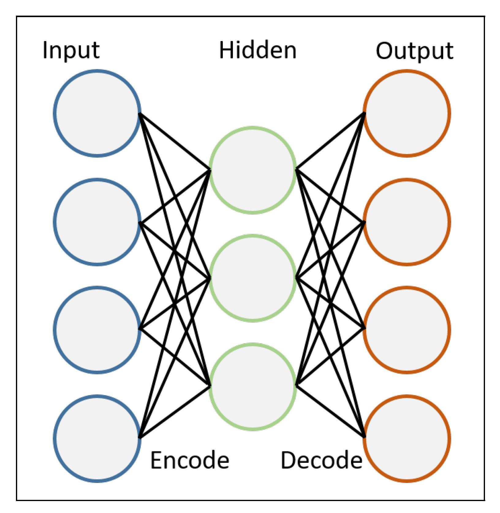
The AE tries to represent the input data by first encoding it, compressing it to the relevant information and decoding it again.
Within the training of the AE, the weights of the neurons are adjusted so that the loss function will yield a minimum. By doing so, the output will represent the input in the best feasible way. In
Figure 1 a general set up of the architecture of the AE can be seen.
Minimizing the loss function:
As mentioned in Vogt et al. [
12], different configurations of AE are possible: An Under Complete Autoencoder (UCA), an DAE or a Contractive Autoencoder (CAE). The implementation that is used within this paper is an UCA that is partly modified. This is more elaborately described in
Section 3.3 3.2. Specifications of the Data Set
The dataset used consists of various offshore WTs located in the same Wind Farm (WF) in the German North Sea. All of them are of the same turbine type with a rated power 5 MW or above. The turbine type is especially designed for offshore usage. The dataset can be subdivided into two different parts: The operational data and the event data. At first, the operational data shall be discussed.
3.2.1. Operational Data
A number of around 300 sensors continuously monitor the performance of each WT. These sensors measure power, wind speed, pressure, temperature, voluminal flow and other values. The WTs are not equipped with sensors that measure the wave height or the salinity of the air. Furthermore, some of the sensors represent counters, e.g., the number of cable windings. Different sampling rates of the sensors are available. Nevertheless, all of the values are grouped into ten-minute-average values by the SCADA-system. For one timestamp with an averaging period of ten minutes, around 300 average values can be seen. A time series consisting of the timestamps is available for every WT. The data available ranges from February 2016 up to December 2019. Next to the average sensor data, an Operational Mode (OM) of each WT is given. The OM is the event triggered and described in the next section.
3.2.2. Event Data: Operational Mode
The OM indicates the state of the WT. This state could be defined as one of the following: Failure, manual stop, service, production, ready. All of the OMs are listed in
Table 1. Only one OM can be valid at a time for one WT. If a new OM is given by the SCADA-systems, the old one will be discarded. Depending on the environmental conditions and the state of the WT, an OM could be present for seconds or several days. To have a complete time series, the discrete events with the information of the WT-state as given by the OM are to be linked to the equidistant operational data. This is described in the next section.
3.2.3. Preparation of the Input Data
Several OMs can appear during an averaging period; e.g., the OM of the WT can be ready, followed by production and end within the same ten minutes in a failure. Nevertheless, only one OM is linked with the equally spaced operational data time series. Therefore, if several OMs are present in one averaging period, only one is chosen depending on an hierarchical order. This order is presented in descending prioritization with the most important OM at the top in
Table 1.
As a result of the concatenation of the operational data and the OMs, an equidistant time series is created where both the information of the sensor values and the information about the WT state is present. This time series is the input for the AE.
Nevertheless, further steps are necessary to have the data ready in that way that it can be used for training. Those steps consist of the following: Dropping of sensors, data imputation and data scaling, filtering for operational modes. These steps are explained subsequently.
Dropping of Sensors
It is to be expected that the time series is complete. Nevertheless, data gaps can be seen. To ensure data quality, filtering for data gaps is conducted. Only if at least 80% of all the values within the training for one sensor are integer or float numbers, this sensor is used further. If it is not the case, the sensor is dropped.
A sensor is also dropped if the value which it represents is a counter and therefore, the values are monotonous rising. Examples are the cable winding, the energy counter or the number of strokes for a specific component. Out of the around 300 sensors, roughly 25 represent counters. Those sensors are dropped.
Data Imputation and Data Scaling
A mean imputation method is chosen for this set up. If the sensor is not dropped but one or more data gaps are still present, the data gaps are substituted with the mean value of all other values of that sensor from this WT. If data gaps occur, they usually can be seen over a period of several days. Linear interpolation between the values before and after the data gap might only partly reflect the sensor behavior. E.g., the fluctuation of the wind within a day. It can be observed that the mean of data gaps regresses to the mean of the sensor with longer data gaps. Therefore with longer data gaps, an imputation with the mean is more appropriated. For data gaps of one hour or less it is expected that a linear interpolation is more appropriate. However this is not yet implemented and therefore part of future work.
Furthermore a standard scaling is implemented to prepare the data to be ready as an usable input for the AE. To standard scale the sensor values its mean value is subtracted and the result is divided by the sensors variance.
Filtering for Operational Modes
One of the reasons for the selection of an AE is that there is less amount of failure data but a high number of normal samples. In this study failure data is present in the form of service reports (see
Section 4.2.1). An average number of 18 reports is issued per WT per operational year. The amount of normal samples per operational year is around 51,000, within one year. This result can be calculated as follows: Every ten minutes within a year one sample (52,560 samples) multiplied with the technical availability given in the literature to be around 96.6% (see Lutz et al. [
17]). An additional reason for a high amount of normal samples can be seen due to the fact that the WT is performing according to its design specifications most of the time. This is also indicated by the time-based availability which is stated to be around 96.6% [
17].
In this study, normal samples are considered to be all the timestamps of the concatenated time series where the operational mode is one of the following: Production, run-up, high-wind shutdown and ready. Furthermore if in the following a normal operational mode is mentioned, it refers to the four mentioned beforehand. Only these operational modes are used for training because they are assumed to represent normal behavior. All other are excluded from training. Purpose of the trained AE is its ability to represent normal behavior of the WT. Any deviation from a normal state for a timestamp given in prediction period is considered to be an anomaly. The training is explained in the next section. The output of the AE in the section afterwards.
3.3. Training the Autoencoder
To train the AE, it is necessary to develop a model architecture. The initial architecture of the AE is as follows: Three hidden layers are used. The first and third of which initially consist of 1350 neurons, the second layer comprises 50 neurons. The input and output dimensions are the same. If in the following the model or an AE is mentioned it refers to the UCA. The input dimensions can vary from one implementation for one WT to another, since some sensors might be dropped. Input dimensions ranging from 243 to 263 dimensions are observed in this set up. The Keras implementation of the adam optimizer, as described in Kingma and Ba [
18] is used. Its learning rate and its decay rate are the same with a value of 0.001. The number of epochs is set to 10. Furthermore, the mini-batch size during the gradient descent executed by the adam optimizer is set to 209 samples. A sample is to be understood as all sensor values for a timestamp after dropping irrelevant sensors. If the input dimension is 263, a sample comprises 263 values, one for each sensor. The selected parameters are visible in
Table 2.
For the activation function, a parametric rectified linear unit is chosen. Its value is set during optimization. With these specifications, the model of the AE is defined, which allows the training process to start.
First, the prepared input data is split into a training set and a validation set. This is done by iterating over the entire dataset and adding 5040 samples (35 days) to the training set and the following 1680 samples (around 12 days) to the validation set. This is repeated subsequently until all available input data out of one year is assigned. It is assumed that a training period of one year is suitable even though shorter or longer periods are possible. Additional research needs to be undertaken in the selection of the most appropriate time window for the training period. However this is part of future work. One year is assumed to be suitable because it contains seasonal dependencies that should be learned as normal behavior by the AE. As stated before four years of operational data are available. Depending on the period in which a prediction is carried out (to be explained in
Section 3.4), different sizes of training periods are available. E.g., in February 2017 one year is available, in February 2018 two years. In order to enable comparable results a training period of one year is selected to train the AE.
Second, the AE is trained on the training set. The training data is mapped to the computed reconstruction and the reconstruction error is optimized. The reconstruction error is to be understood as the difference between the input data and the reconstruction. Additionally, the AE will also map the validation data, which is not part of the training data to its reconstructions, followed by another reconstruction error computation. The mean reconstruction error over the validation data then is yielded as a value, which later can be used to rate the performance.
Once the AE is trained, it is able to reconstruct the sensor values for a given input. To express if the input is abnormal or normal, we first compute the reconstruction error again. Modeling the reconstruction error as a vector of random variables leads to different methods to measure the abnormal behavior of the input based on the reconstruction error. This is described in the next paragraph.
Measure the Reconstruction Error
Using the RMSE to measure the reconstruction error, implicitly assumes that the sensor values are independently distributed. Under the assumption that some sensors are not independent of each other, the Mahalanobis distance (see Equation (
4)) is used.
This measure uses the covariance matrix of the random variables to take possible dependencies into account. Furthermore, it provides a more realistic measure for this case. Since the covariance matrix of the random variables is unknown, it will be estimated from the given dataset. Using a standard covariance estimator may lead to a wrong result caused by outliers in the dataset. Therefore an outlier robust covariance estimation is used as described in Butler et al. [
19]. It approximates the covariance matrix of the random variables iteratively. After estimating the covariance, it is now possible to compute the Mahalanobis distance of every input sample and use it as a score, which determines how abnormal the reconstruction error of a given sample is.
Mahalanobis distance:
where:
By using this measure for each input sample x, a value for the score can be calculated. If this value is higher than a chosen threshold (
) the input sample is considered to be an abnormal one. This is seen in Equation (
5) and also mentioned in Vogt et al. [
12].
To calibrate the value for the threshold, one has to consider the predictions ground truth. Four different possibilities can be concluded if the predictions for an anomaly are compared to the actual OM. This is seen in
Table 3.
With these four possible outcomes, the false discovery rate (see Equation (
6)) can be defined. This value expresses how many of the sample scores above the threshold are normal according to the OM
False discovery rate:
where:
This allows calibration of the threshold. At first, all scores of the training and validation dataset are calculated and sorted in ascending order. By iterating over all possible thresholds from 0 to the maximum of all calculated scores, the threshold can be calibrated. For each possible threshold the fdr (see Equation (
6)) is calculated. The first threshold is chosen, where the false discovery rate is lower than the selected value. With the value for the fdr selected, it can be guaranteed that the selected percent of all detected samples are normal according to the OM. In this case, the fdr is selected to be
. Thereby a higher sensitivity is given and timestamps are more easily considered to be abnormal. This is a desired behaviour since the impact of subsequent abnormal timestamps form the basis for another measure. This measure is described in Equation (
7).
3.4. Using the Trained Model
The input data for the training of the AE consists out of operational data for a consecutive time of one year. Once the AE is trained and the threshold calibrated, a prediction can be made for new timestamps. It is referred to as prediction period in the following. Since the operational data (see
Section 3.2.1) is available starting from February 2016, the earliest prediction can be made by February 2017. The time window for the prediction period is set to a window of seven days.
A time window of seven days is chosen out of the following reasons:
First, after performing maintenance actions at the WT it is regularly seen that some parameters of the WT differ. E.g., Oil has been refilled or some control parameters are adjusted. This leads to a changed behaviour of the WT. Yet this behaviour is within design specifications, the AE has not learned it while training and therefore it is more likely to observe an extended amount of anomalies after a maintenance action.
Second, a focus of this tool is to give decision support in a scenario where in a daily routine at several WTs preventive measures are necessary to perform. If one of the WT is more likely to fail, preventive measures need to be carried out first. With limited resources the question arises which WT should be prioritized. This tool helps in making this decision easier by identifying the WT which is more likely to fail. A prediction period of more than seven days might also be appropriate. Nevertheless the authors did not investigate this matter. It is part of future work.
For each timestamp in the prediction period, the score can be calculated (see Equation (
4)). If the value for the score is above the calibrated threshold, an anomaly is detected. This boolean result is available for any timestamp in the prediction (see Equation (
5)). To assess the impact of subsequently arising anomalies, a further measure is defined: The criticality. It is a counter that rises by one if an anomaly is detected and a normal operational mode is present for that timestamp. The criticality decreases by one if no anomaly is detected. It stays constant if the operational mode for that timestamp is a service and an anomaly is detected. Its lower limit is zero and its upper level is equal to the number of timestamps in the prediction time window, which is 1008 instances. This implies an anomaly for every timestamp within seven days.
The value of the criticality within the time window of the prediction period is selected as a criteria to evaluate the failure detectability of the AE. It is described in Equation (
7).
With
being the timestamps for the prediction period. The results by applying this equation are outlined in
Section 5. Before doing so, a set of standardized failures has to be prepared. This is explained in the section that follows.
4. Preparation of a Clean Failure Data Set
Maintenance information about the WT is available in the form of service reports. Different maintenance engineers have described their activities at the WT-site. For each action, a text description is given, which also indicates the start and the end of the WT unavailability. Since different engineers use varying semantics for the same WT-subsystems the maintenance information needs to be standardized (see
Section 4.2.1 and
Section 4.2.2). Before that, downtime events are explained. They serve as a tool to validate the unavailability documented in the reports. This is described in the following section.
4.1. Generation of Downtime Events
With the ten-minute average values of the sensors wind speed and power calculations and assumptions can be made. Since this calculation is rather an input to validate events it will be referred to as event data. Given the wind speed and the power for each timestamp, a decision can be made for the overall state of the WT. Wind speed and power are to be understood, as explained in the standard IEC 61400-25 [
20]. The scada-events are outlined in
Table 4.
With the values for wind speed and power given for each timestamp, a scada-event can be deduced. If the scada-event is the same for several sequential timestamps they will be joined together to one event. The beginning of the first timestamp indicates the start. The end of the last timestamp indicates the end of the event. This is what is to be understood if in the following a scada-event is mentioned. Within an averaging period the turbine could be both: Producing energy and consuming energy e.g., due to a cable unwinding. Hence if the values for power are averaged, this information can hardly be accessed. Nevertheless, the boundaries for wind speed and power for the different scada-events are choosen according to
Table 4.
4.2. Description and Standardization of Failures
4.2.1. Event Data: Service-Reports
The scada-events provide the information if the WT is in downtime. But it does not resolve the question of why a downtime has happened. Several causes for downtime of a WT exist. It can be due to a regulation action: e.g., load curtailment, noise reduction shutdown or bird conservation actions. Furthermore, a downtime can occur if preventive or corrective measures are being performed at the WT. If so a service report will be issued by the service provider to the operator. Within this report, a detailed description of the work performed by the service team is written down. This text will describe the type of maintenance measure and which component has been the subject of the work. The service reports with a text description of the work performed are available for evaluation. A service report is available if during a maintenance activity the onboard crane system of the WT can be used for the carriage of materials for exchange, repair or enhancement of WT components or if only persons are performing measures at the WT. If the material is too heavy to be lifted with the onboard crane, no service report is available for the evaluation, as described in this paper. Different enterprises are involved and another form of documentation is used, which is not obtainable to the authors.
Since the text descriptions contained in the service report is hard to use for analysis described in
Section 5 they need to be standardized. This is going to be outlined in
Section 4.2.2. Next to the text description other information is also provided in the service-report. This information implies the start and end of the measure at the WT, the start and end of the unavailability, the material consumption, the technicians, the tools used, an identifier for the WT next to other details.
4.2.2. Standards
Two structures shall be introduced in the following: Reference Designation System for Power Plants® (RDS-PP®) and Zustand-Ereignis-Ursachen-Schlüssel (Engl: State Event Cause Code) (ZEUS). These structures will be used to classify the text description into standards.
RDS-PP®
The standard RDS-PP
® aims at having a unique structure of WT systems and subsystems and a hierarchically dependency of those systems amongst each other. An example: On RDS-PP
® level 1 all of the components related to the WT and its subsystems will be referred to as wind turbine systems. Beneath the wind turbine system on level 2, the yaw system, the drive train system and the rotor system are structured next to others. Two advantages of the standard shall be mentioned: First, the standard can be used to compare different WTs of different Original Equipment Manufacturer (OEMs) and second the components can be grouped into subsystems and systems. The first one does not apply in this paper since one WF with WTs of the same turbine type is the subject of consideration. Nevertheless, the second benefit applies and is being used and described in
Section 5.
ZEUS
ZEUS is introduced by the Fördergesellschaft Windenergie und andere Dezentrale Energien (FGW) within the technical guideline TR7 [
21]. ZEUS introduces several blocks that describe the state of the turbine and the state of a component. With the combination of all blocks nearly every state of the WT is defined. Each block raises a question that is answered by a certain code in the sub-block. An example: In ZEUS Block 02-08 the question is raised “Which type of maintenance is active or will be necessary to eliminate a deviation from the target state?”. This answer can be given by the ZEUS-code 02-08-01, which is corrective maintenance or by the ZEUS-code 02-08-02, which indicates preventive maintenance. For a better understanding about the terminology of preventive and corrective see the British Standards Institution: Maintenance–Maintenance terminology [
22].
4.3. Selection of Failures
In order to investigate only the corrective maintenance events, filtering is done according to ZEUS. Only those events are selected where a failure has happened or the measure to restore the WT to a functional state is a corrective one. Those events are further used in
Section 5. The detected anomalies before such events will be evaluated. Therefore only the events with the ZEUS block shown in
Table 5 are chosen.
If an event fulfills one of the criteria shown in
Table 5, it is selected. Thereafter it has to be validated with the downtime events. This is described in the next chapter.
4.4. Validation of Failures with Downtime Events
Having created scada-events and a set of standardized failures (see
Section 4.1 and
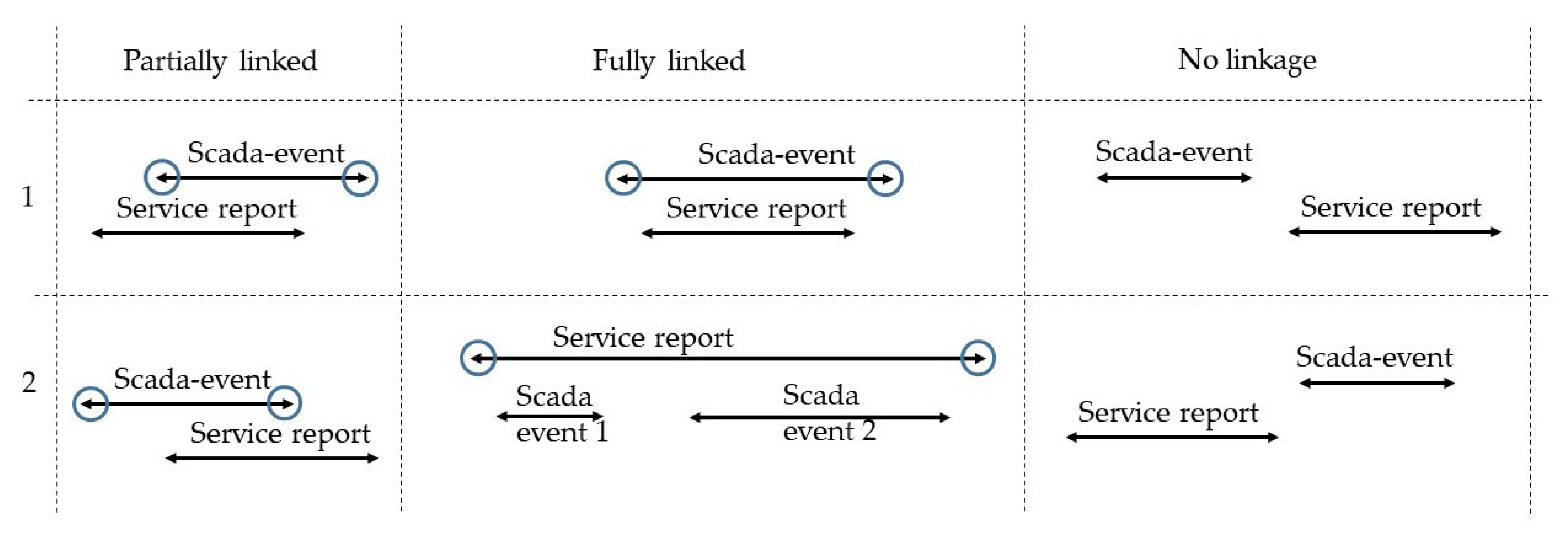
Section 4.2), it is necessary to validate whether a failure resulted in a downtime of the corresponding WT. Therefore, the start and the end of the unavailability as indicated in the service-reports are compared with the beginning and the end of the scada-events. It is to be expected that the downtimes of the service reports could be related to the scada events. Nevertheless, three different cases could be observed: A partial linkage, a full linkage and no linkage at all. These three different cases can be seen in
Figure 2.
If the downtimes do not match, but overlap, the start and the end of the scada event, as indicated by the blue circles, are used within the clean failure dataset (e.g., partially linked
Figure 2). If a service report does not overlap with the scada event, the single events are excluded from the clean failure set (e.g., no linkage in
Figure 2).
As a summary, it can be stated that 35% of the events showed a full linkage, 41% showed partially linkage and 24% could not be linked and, therefore, have been removed from further analysis. No linkage is done if the WT is operating during the service. Furthermore, different entries for dates are available: The date the service report is issued and the date the service duty has happened. If the entry for the date of the service duty is not available the date of the issuing is used. This may lead to no linkage of the scada-event with the report.
Some 1495 reports have been standardized. After filtering by ZEUS, 799 of those reports remain, which are considered to indicate corrective maintenance.
5. Evaluating the Failure Detectability of the Autoencoder
In this section, the trained AE is executed on a time window of seven days: The prediction period. The maximum of the criticality, as described in Equation (
7) is chosen to compare and to group the different prediction periods. Two different scenarios are considered. At first the period of expected normal operation (ENO) is discussed (see
Section 5.1). At second, a period before the day of a known historical failure (see
Section 5.2). The result and the comparison of the two are shown in
Section 5.3.
5.1. Anomalies during Expected Normal Operation
An assumption is to be made of what is considered to be ENO. A time of three weeks in which the WT is in a normal OM the majority of the time. Therefore each day, the number of timestamps with a normal OM is counted. If the number of normal OMs is greater or equal to 138 for every single day within three weeks, a period of ENO is identified. Within those three weeks, operational modes that indicate service or error could be present, e.g., a reset of the WT but not longer than for one hour a day. Of those three weeks of ENO, the second week is selected as the period of prediction. For each WT two of those periods are identified to have the same amount of events as described in the next section.
5.2. Anomalies before Known Failures
109 reports remain after filtering for the beginning of data acquisition of one year and seven days before the failure has occurred. The evaluation is done for all of those remaining failures. The failures are described briefly: The majority was detected in the rotor system, followed by the control system and the converter system. These three systems are often ranked the highest in terms of failure occurrence. This can also be seen in Pfaffel et al. [
23]. The average downtime of the failures considered is close to 2.5 days. The shortest downtime has a value of around 30 min, the most extended downtime a value of approximately 22 days. The anomalies before the 109 known failure are to be observed and the criticality calculated. The last day of the prediction period contains the downtime of the failure.
5.3. Potential Detectability of Wind Turbine Failures
Before the detectability of the failures is discussed, the criticality is to be grouped into different ranges. This is described in the next section.
5.3.1. Potential Scheduling Time
The ranges reflect the possible scope of action of the operators and are based on the authors’ interpretations. The interpretations are seen in
Table 6. If the value for the criticality is 0, the failure detectability is interpreted as no detection. If the criticality is greater than 432 in the prediction period of seven days, the detectability can be construed as a reliable detection. The different ranges of the criticality shown in
Table 6 are further used to group the maximum of the criticality of the prediction periods of the two different scenarios (see
Section 5.1 and
Section 5.2). The results can be seen in
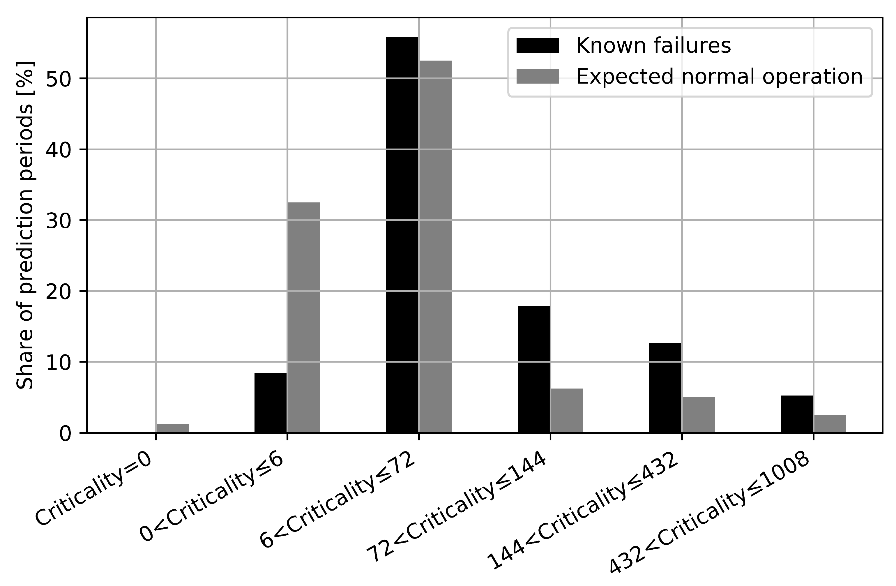
Figure 3.
Figure 3 shows the maximum of the criticality in the different prediction periods. The black bars represent the prediction periods in which, on the last day, a failure has happened. The grey bars represent the prediction periods in which the WT is in ENO. The maximum of the criticality in the prediction period is grouped into different ranges (see
Table 6) and divided by the total number of prediction periods in the scenario (Failure or ENO). By doing so, the share of the prediction periods can be displayed on the
y-axis. In
Figure 3 one can see that the black bars are more dominant at values for a higher criticality. Grey bars are more present at values for a low criticality. This underlines the capability that more anomalies are raised in periods where failure is about to happen. Furthermore, if one only considers the grouped bars for the criticality of 72 or higher it can be concluded that the black bars are almost double in their percentage value compared to the grey bars. It can be interpreted as the probability of a failure to happen is two times higher than a period of ENO to appear. Almost one-third of the prediction periods with a known failure are in this range with a criticality of 72 or higher.
It can be stated that more anomalies can be seen in periods where a failure has happened. Nevertheless, some periods of ENO show a high criticality. Several reasons could explain such a behavior: Within a reset of the WT some control parameters are changed or before the period of ENO a longer service was conducted. This leads to a new WT behavior, which has not been seen in the training, and therefore anomalies are detected.
In the next section the subsystems that are subject to expected long term detection and reliable detection (ELT&RD) (see ranges in
Table 6) are to be discussed. Furthermore, some of those prediction periods are further investigated.
5.3.2. Potential Detectability of Wind Turbine Component Failures
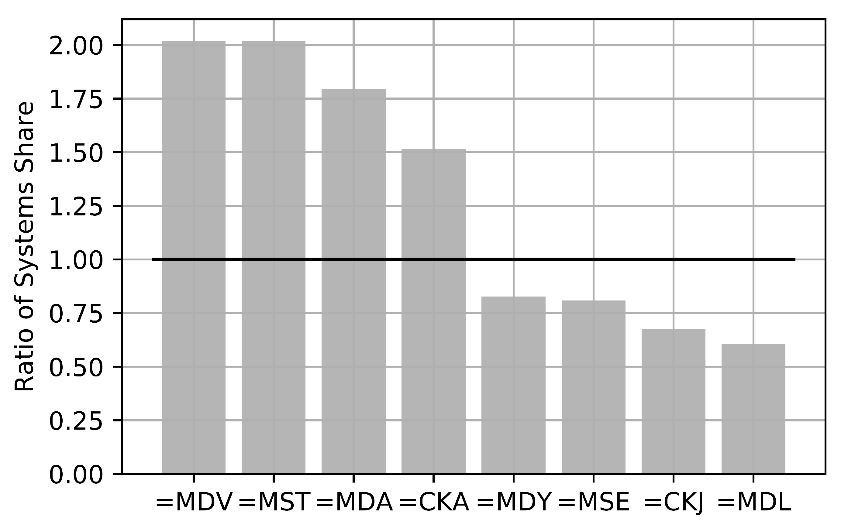
Anomalies can be seen before failures have happened in different WT-systems.
Figure 4 shows the ratio of systems share. The proportion of failures in RDS-PP
® systems that are related to ELT&RD is calculated. Similar, the proportion was calculated for all RDS-PP
® systems that are available for evaluation after filtering (see
Section 5.2). These two proportions are divided. The result will yield a ratio for each RDS-PP
® system. It is displayed in
Figure 4 on the
y-axis and its calculation is given in Equation (
8). The ratio indicates if the detectability of failures (ELT&RD) has increased or decreased if compared to the share of all possible detectable failures.
where:
| Number of failures in specific RDS-PP® system subject to ELT&RD |
| Number of failures in specific RDS-PP® system. All failures available for evaluation considerd. |
| Ratio | Ratio of systems share |
| n | Number of unique RDS-PP® systems subject to ELT&RD |
| m | Number of unique RDS-PP® systems available for evaluation |
On the x-axis, the systems on RDS-PP® level 2 are visible: The central lubrication system (=MDV), the generator transformer system (=MST), the rotor system (=MDA), the fire alarm system (=CKA), the control system (=MDY), the converter system (=MSE), the environmental measurement system (=CKJ) and the yaw system (=MDL).
It can be deduced that failures in the central lubrication system, the generator transformer system and the rotor system are possible better to detect. Those systems are overrepresented in failures that are considered to be ELT&RD. The ratio increases by around two. The opposite applies to failures, which happen in the converter system (=MSE), the environmental measurement system (=CKJ) and the yaw system (=MDL). Here a decrease of the ratio is seen. A ratio of one would indicate that the share of systems (ELT&RD) compared to all systems considered did not change, yet this is not recognized.
In
Figure 5, the development of the criticality over the timestamps in the prediction period is visualized. On the last day of the prediction, failure is seen. The time of constant criticality indicates the OM service, which happened after a failure is detected at the WT. The failures shall be discussed briefly. An anomaly is almost present in every timestamp in the prediction period before a failure showed up in the central lubrication system (=MDV). The amount of grease was low and therefore had to be refilled. This caused a shutdown of the WT. Similar behavior of the criticality is seen before a failure appeared in the rotor system (=MDA). Some adjustments of connectors needed to be made. In the case of the failure in the meteorological measurement system (=CKJ) many anomalies are detected as well. Here both of the anemometers had to be replaced during the service after the failure.
6. Discussion
The model of the AE was taken from Vogt et al. [
12] and further developed. A hyper parameter optimization (HPO) is not implemented for every model. Rather, the best parameters of one model are selected to be valid for all other models as well. A HPO should be part and further explained in future work. As for now, the false discovery rate is chosen to select the best value for the threshold. Part of future research should probably be to apply and test different methods to calibrate the threshold. Furthermore, different time windows for the prediction period need to be investigated. Additional work should also focus on different imputation methods for different lengths of data gaps and for sensors with varying characteristics in terms of the system inertia which they are measuring. The implementation of an AE, based on the proposed methodology, on WT data is especially helpful to detect anomalies that are rather dynamic. To also investigate long term trends, a system needs to be combined with the AE developed.
By using an AE, it is possible to identify abnormal WT behaviour. Nevertheless, domain knowledge is still needed to validate if an anomaly is likely to turn into a failure. Furthermore, it is still required to identify which system, subsystem or component is the root cause for the detected anomaly. Additional research will also focus on identifying not only the WT, which is critical, but also the sensor or set of sensors that are most probably causing the anomaly. This will lead to ease of decision making.
Three assumptions are to be mentioned:
It is to be expected that the WT is performing according to its design specification most of the time and a training of the AE will represent normal behaviour.
It is expected that deviations from a normal state can be seen in the ten-minute-average data of the sensors and the operational data, and this is indicated as an anomaly by the trained AE.
It is expected that the information in the service reports and the descriptions of the work performed are correct and standardized correctly.
7. Summary and Outlook
The AE developed here shows a good possibility to detect historical failures in various WT-systems. This can be deduced because many anomalies are seen before a failure has happened. At first, the AE is developed, and secondly, the failures are structured and standardized according to RDS-PP® and ZEUS. After doing so, those two approaches were linked and the detectability of failures with the AE were validated on a set of standardized historical failures. Of all the failures, around 35.7% were subject to likely midterm detection, which can be interpreted as at least six hours of constant anomalies. About 17.8% of all failures are considered as expected long term detection, which can be understood as at least 24 h of constant anomalies. About 5.2% can be detected reliably. This can be interpreted as at least 72 h of constant anomalies. By standardizing the failures, we can state which system failures are more easily detectable. These systems were as follows: The central lubrication system, the generator transformer system and the rotor system.
The usage of an AE could help to identify failures and upcoming repair measures in various WT-systems and thereby to increase the revenue and the uptime of the WT by a significant extent.
Author Contributions
Conceptualization, M.-A.L., U.S.; methodology, M.-A.L., U.S., A.O.; software, M.-A.L., S.V., C.G., A.O.,; validation, M.-A.L.; formal analysis, M.-A.L.; investigation, V.B.; resources, M.-A.L., V.B., U.S.; data curation, S.D.; writing—original draft preparation, M.-A.L., V.B., U.S., C.G., A.O.; writing—review and editing, M.-A.L.; visualization, M.-A.L.; supervision, V.B., S.F.; project administration, V.B., S.F.; funding acquisition, V.B., S.F. All authors have read and agreed to the published version of the manuscript.
Funding
The research work presented in this paper was funded by the German Federal Ministry for Economic Affairs and Energy through the research project ModernWindABS under grant number 0324128.
Conflicts of Interest
The authors declare no conflict of interest. The funders had no role in the design of the study; in the collection, analyses, or interpretation of data; in the writing of the manuscript, or in the decision to publish the results.
Abbreviations
The following abbreviations are used in this manuscript:
| AE | Autoencoder |
| ANN | Artificial Neural Network |
| CAE | Contractive Autoencoder |
| CMS | Condition Monitoring System |
| DAE | Denoising Autoencoder |
| DDM | Data Driven Model |
| ELT&RD | Expected Long Term Detection and Reliable Detection |
| ENO | Expected Normal Operation |
| FGW | Fördergesellschaft Windenergie und andere Dezentrale Energien |
| HPO | Hyper Parameter Optimization |
| LCOE | Levelized Cost of Energy |
| MTTR | Mean Time to Repair |
| NBM | Normal Behaviour Model |
| OEM | Original Equipment Manufacturer |
| OM | Operational Mode |
| O&M | Operation and Maintenance |
| ROC | Receiver Operation Characteristic |
| RDS-PP® | Reference Desigantion System for Power Plants® |
| SCADA | Supervisory Control and Data Acquisition |
| SHM | Structural Health Monitoring System |
| UCA | Under Complete Autoencoder |
| WF | Wind Farm |
| WT | Wind Turbine |
| ZEUS | Zustand-Ereignis-Ursachen-Schlüssel (Engl: State Event Cause Code) |
References
- Lei, X.; Sandborn, P.; Bakhshi, R.; Kashani-Pour, A.; Goudarzi, N. PHM based predictive maintenance optimization for offshore wind farms. In Proceedings of the IEEE/Conference on Prognostics and Health Management 2015, Austin, TX, USA, 22–25 June 2015; pp. 1–8. [Google Scholar] [CrossRef]
- Wang, H. A survey of maintenance policies of deteriorating systems. Eur. J. Oper. Res. 2002, 139, 469–489. [Google Scholar] [CrossRef]
- Stephan, M.; Steinmetz, U.; Schinsky, J. Zusätzliche Einnahmen aus Windparks durch Verbesserte Datenanalyse; VGB Powertech: Essen, Germany, 2015; pp. 62–67. [Google Scholar]
- Bangalore, P.; Tjernberg, L.B. An Artificial Neural Network Approach for Early Fault Detection of Gearbox Bearings. IEEE Trans. Smart Grid 2015, 6, 980–987. [Google Scholar] [CrossRef]
- Liu, W.Y.; Tang, B.P.; Han, J.G.; Lu, X.N.; Hu, N.N.; He, Z.Z. The structure healthy condition monitoring and fault diagnosis methods in wind turbines: A review. Renew. Sustain. Energy Rev. 2015, 44, 466–472. [Google Scholar] [CrossRef]
- Martinez-Luengo, M.; Kolios, A.; Wang, L. Structural health monitoring of offshore wind turbines: A review through the Statistical Pattern Recognition Paradigm. Renew. Sustain. Energy Rev. 2016, 64, 91–105. [Google Scholar] [CrossRef] [Green Version]
- Lau, B.C.P.; Ma, E.W.M.; Pecht, M. Review of offshore wind turbine failures and fault prognostic methods. In Proceedings of the IEEE 2012 Prognostics and System Health Management Conference (PHM-2012 Beijing), Beijing, China, 23–25 May 2012; pp. 1–5. [Google Scholar] [CrossRef]
- Helbing, G.; Ritter, M. Deep Learning for fault detection in wind turbines. Renew. Sustain. Energy Rev. 2018, 98, 189–198. [Google Scholar] [CrossRef]
- Zaher, A.; McArthur, S.; Infield, D.G.; Patel, Y. Online wind turbine fault detection through automated SCADA data analysis. Wind Energy 2009, 12, 574–593. [Google Scholar] [CrossRef]
- Schlechtingen, M.; Ferreira Santos, I. Comparative analysis of neural network and regression based condition monitoring approaches for wind turbine fault detection. Mech. Syst. Signal Process. 2011, 25, 1849–1875. [Google Scholar] [CrossRef] [Green Version]
- Zhao, H.; Liu, H.; Hu, W.; Yan, X. Anomaly detection and fault analysis of wind turbine components based on deep learning network. Renew. Energy 2018, 127, 825–834. [Google Scholar] [CrossRef]
- Vogt, S.; Berkhout, V.; Lutz, A.; Zhou, Q. Deep Learning Based Failure Prediction in Wind Turbines Using SCADA Data. In Proceedings of the 4th Conference for Wind Power Drives 2019, Aachen, Germany, 12–13 March 2019. [Google Scholar]
- Deeskow, P.; Steinmetz, U. Prädiktive Instandhaltung auf Basis von Big Data und Machine Learning: Monitoring mit Plus an Intelligenz, Effizienz und Wirtschaftlichkeit. Ew Magazin für die Energiewirtschaft 2019, 7–8, 46–50. [Google Scholar]
- Jiang, G.; Xie, P.; He, H.; Yan, J. Wind Turbine Fault Detection Using a Denoising Autoencoder With Temporal Information. IEEE/ASME Trans. Mechatron. 2018, 23, 89–100. [Google Scholar] [CrossRef]
- Wu, X.; Jiang, G.; Wang, X.; Xie, P.; Li, X. A Multi-Level-Denoising Autoencoder Approach for Wind Turbine Fault Detection. IEEE Access 2019, 7, 59376–59387. [Google Scholar] [CrossRef]
- Odgaard, P.F.; Johnson, K.E. Wind turbine fault detection and fault tolerant control—An enhanced benchmark challenge. In Proceedings of the American Control Conference (ACC) 2013, Washington, DC, USA, 17–19 June 2013; IEEE: Piscataway, NJ, USA, 2013; pp. 4447–4452. [Google Scholar] [CrossRef]
- Lutz, M.A.; Görg, P.; Faulstich, S.; Cernusko, R.; Pfaffel, S. Monetary–based availability: A novel approach to assess the performance of wind turbines. Wind Energy 2019, 56, 226. [Google Scholar] [CrossRef] [Green Version]
- Kingma, D.P.; Ba, J. Adam: A Method for Stochastic Optimization. arXiv 2014, arXiv:1412.6980. [Google Scholar]
- Butler, R.W.; Davies, P.L.; Jhun, M. Asymptotics For The Minimum Covariance Determinant Estimator. Ann. Stat. 1993, 1993, 1385–1400. [Google Scholar] [CrossRef]
- International Electrotechnical Commission. 61400-25-2: Communications for Monitoring and Control of Wind Power Plants—Information Models: 2016-06; International Electrotechnical Commission: Geneva, Switzerland, 2016. [Google Scholar]
- Fördergesellschaft Windenergie und andere Dezentrale Energien. TG 7—Technical Guidelines for Power Generating Units—State-Event-Cause Code for Power Generating Units (ZEUS) Rubric D2—Maintenance of Power Plants for Renewable Energy, Category D2: State-Event-Cause Code for Power Generating Units (ZEUS)—Terms, Classification and Structuring of States, Events, Causes and Measures for Future Assessments and Improvements in Operation and Maintenance; Fördergesellschaft Windenergie und andere Dezentrale Energien: Berlin, Germany, 1 October 2013. [Google Scholar]
- British Standards Institution. Maintenance—Maintenance Terminology; Technical Report 13306; British Standards Institution: London, UK, 2010. [Google Scholar]
- Pfaffel, S.; Faulstich, S.; Rohrig, K. Performance and Reliability of Wind Turbines: A Review. Energies 2017, 10, 1904. [Google Scholar] [CrossRef] [Green Version]
© 2020 by the authors. Licensee MDPI, Basel, Switzerland. This article is an open access article distributed under the terms and conditions of the Creative Commons Attribution (CC BY) license (http://creativecommons.org/licenses/by/4.0/).

 ,
, 


