Magnetic Positioning Technique Integrated with Near-Field Communication for Wireless EV Charging

Abstract

For wireless electric vehicle charging, the relative position of the primary and secondary coils has significant impacts on the transferred power, efficiency and leakage magnetic flux. In this paper, a magnetic positioning method using simultaneous power and data transmission (SWPDT) is proposed for power coil alignment. Four signal coils are installed on the primary coil to detect the secondary coil position. By measuring the positioning signal amplitudes from the four signal coils, the power coil relative position can be obtained. Moreover, all the communication needed in the positioning process can be satisfied well by SWPDT technology, and no extra radio frequency (RF) communication hardware is needed. The proposed positioning method can work properly both in power transfer online condition and in power transfer offline condition. Thus, a highly integrated wireless charging system is achieved, which features simultaneous power transfer, data transmission and position detection. A positioning experimental setup is built to verify the proposed method. The experimental results demonstrate that the positioning resolution can be maintained no lower than 1 cm in a 1060 mm × 900 mm elliptical region for a pair of 510 mm × 410 mm rectangular power coils. The three-dimensional positioning accuracy achieves up to 1 cm.

1. Introduction

Wireless electric vehicle charging (WEVC) is gaining worldwide attention and developing very quickly [1,2,3]. Compared to the conductive charging method, WEVC eliminates the bulky cables, the requirement of a manual connection, and the associated hazards. WEVC exhibits many attractive advantages such as convenience, safety and weatherproofing. Both inductive power transfer (IPT) and capacitive power transfer (CPT) can be used for WEVC [3]. This paper is focused on the IPT system.

For IPT systems, the coil misalignment greatly deteriorates the transferred power, efficiency and leakage of magnetic flux [3,4]. Much research to improve the misalignment tolerance of IPT systems has been conducted [5,6,7,8,9,10,11,12]. The preferred approach is to optimize the coil structure [5,6,7], which maintains a relatively uniform magnetic field distribution during misalignment. Another approach is to optimize the compensation network, which improves the circuit performance under misalignment conditions [8,9,10,11,12]. However, the improvement of misalignment tolerance is limited, and the charging still needs to take place in a limited charging zone. To confirm the pickup coil being within the charging zone, the position detection of power coils is indispensable for a practical wireless charger, as described by SAE J2954 [13]. On the other hand, if the position detection method is of high accuracy, it can be combined with the autonomous parking technology to align the power coils accurately. This will reduce the need to design an IPT system with large misalignment tolerance. Accordingly, the extra hardware cost and control cost for the misalignment tolerance improvement can be reduced. Therefore, for a commercialized wireless EV charger, the cost of improving position detection accuracy and the cost of improving misalignment tolerance should be traded off.

Some position detection methods available on the market have been considered for WEVC, such as radio frequency (RF) positioning [14,15,16,17,18,19,20], optical positioning [21,22] and acoustical positioning [23]. However, RF positioning and acoustical positioning both suffer signal multipath impairment and non-line-of-sight impairment when they work in a complex environment. The optical positioning methods, including visual image analysis and infrared positioning, are susceptible to obstacles, dust and harsh weather. Meanwhile, all the methods above are limited by their high cost and difficulty in integrating with the power pads. Magnetoresistive (MR) sensors are investigated to be used for coil misalignment detection [24,25,26,27], but this method has not achieved precise three-dimensional (3D) coordinate output, and plenty of sensors involved in the sensor matrix greatly increase the system cost and complexity. Moreover, some magnetic positioning methods are proposed in [28,29,30,31,32,33], which utilize auxiliary coils to measure the magnetic field generated by the primary power coil. The magnetic positioning methods are of high accuracy, low cost, not susceptible to the environment and are easy to integrate with power pads. In [28,29,30,31,32,33], the primary power coil needs to generate a very weak magnetic field for positioning. Thus, the primary resonant tank is excited by a very low-voltage source during positioning. For this very low-voltage mode, the primary high-power inverter has to switch to a very low direct current (DC) bus voltage [31,32], or to operate with a very large phase-shift angle [33]. However, either the added bus selection switches or the large phase-shift operation will decrease the reliability and safety of the high-power inverter. Moreover, the inverter can only work in the high voltage mode for power transfer, or the low voltage mode for positioning at a time. Thus, position detection and power transfer cannot be simultaneously conducted, i.e., the online position monitoring is impossible.

We have proposed a simultaneous wireless power and data transmission (SWPDT) system in [34], which is based on the frequency division multiplexing (FDM) technique and quadrature phase-shift keying (QPSK) modulation. A high-frequency data carrier is modulated by four discrete phase shifts to represent two binary bits. The data carrier is injected into one side of the IPT system, and then it transfers to the other side through the magnetic coupling between power coils. The data carrier is then extracted and demodulated, so that the near-field communication can be achieved. In this method, the amplitude of the data carrier is not utilized for communication purpose. However, the receiving amplitude of the data carrier is proportional to the mutual inductance between power coils, which means it contains the relative position information of power coils. Unfortunately, the three-dimensional (3D) position cannot be determined exactly by only one mutual inductance. Thus, more independent mutual inductances should be involved to derive the 3D coordinate. This idea has been revealed in our preliminary work [35].

Based on the near-field communication technology in SWPDT, this paper proposes a magnetic positioning method, which has the following features:

(1) Four auxiliary signal coils are added for positioning while other hardware is shared with the SWPDT system.

(2) The positioning signal is transmitted by the signal coils rather than the primary power coil, so the very low voltage mode of the high-power inverter, as mentioned before, is avoided.

(3) The positioning process can be carried out both in the power transfer online condition and in the power transfer offline condition. The proposed amplitude measurement method is immune to the power fundamental interference and ensures online positioning accuracy.

(4) The communication need in the positioning process can be well satisfied by SWPDT technology. A highly integrated IPT system for WEVC is achieved, i.e., simultaneous power transfer, data transmission and position detection.

2. Magnetic Positioning Integrated with Near-Field Communication in Simultaneous Wireless Power and Data Transmission (SWPDT) System

2.1. Communication Principle of SWPDT System

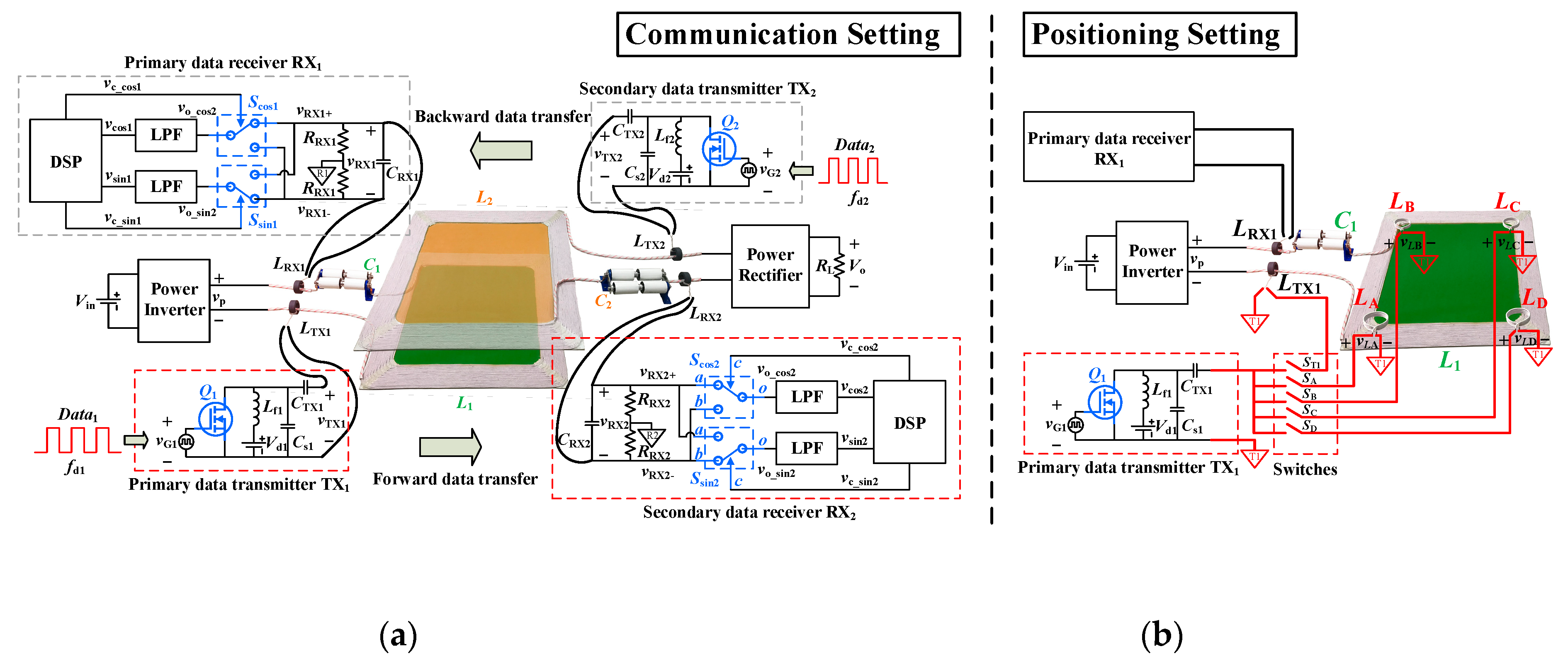
The original SWPDT system proposed in [34] is shown in Figure 1a, and labelled as “communication setting” in this paper. The subscripts “1” and “2” stand for the primary side and the secondary side, respectively. The forward communication channel can be expressed as TX₁→L_TX1→L₁→L₂→L_RX2→RX₂, where L_TX1 is used to inject the data carrier into the power circuit, and L_RX2 is used to extract the data carrier from the power circuit. Similarly, the backward communication channel is TX₂→L_TX2→L₂→L₁→L_RX1→RX₁. The configurations of the forward communication and the backward communication are fully symmetrical. The only difference is that they use two different data carrier frequencies, i.e., f_d1 (5 MHz) for the forward and f_d2 (6.25 MHz) for the backward. Thus, the forward communication is illustrated as an example in the following.

For the primary data transmitter TX₁, the switching frequency of Q₁ is equal to the data carrier frequency f_d1. The gate drive signal v_G1 is modulated with four kinds of phase shift φ, i.e., 0, π/2, π, 3π/2, as shown in Figure 2 [34]. The transmitting signal v_TX1 with each phase shift for a certain duration T_symbol is called a symbol. As shown in the mapping table of Figure 2, the data is represented by the phase change Δφ between two adjacent symbols, namely differential quadrature phase-shift keying (DQPSK). The transmitting signal v_TX1 and the adjacent phase change Δφ can be expressed by:

$$v_{\mathrm{TX}1}(t)=A_1\sin \left(2\mathsf{\pi }{f}_{\mathrm{d}1}t+\phi (n)\right),\phi (n)\in \left\{0,\mathsf{\pi }/2,\mathsf{\pi },3\mathsf{\pi }/2\right\},$$

(1)

$$\Delta \phi (n)=\phi (n)-\phi (n-1),$$

(2)

where A₁ is the constant amplitude, and n is the symbol sequence number.

The transmitting signal v_TX1 is injected into the power circuit by the loose coupling between L_TX1 and the power line, and then transfers to the secondary side through the coupling of power coils L₁L₂. The receiving capacitor C_RX2 is resonant with the signal extractor L_RX2 at the data carrier frequency f_d1, which forms a narrow passband filter to extract the data carrier f_d1. The data signal received on C_RX2 can be expressed by:

$$v_{\mathrm{RX}2}(t)=K_{12}{A}_1\sin \left(2\pi f_{\mathrm{d}1}t+\phi (n)+{\phi }_{12}\right),$$

(3)

where K₁₂ and φ₁₂ are the forward transfer gain and phase shift, respectively. K₁₂A₁ is the receiving signal amplitude, which is denoted as |V_RX2|.

Through the demodulation circuit in RX₂, the adjacent phase change Δφ(n) can be calculated by (4) [34]. Then the data can be demodulated according to the mapping table in Figure 2, so that the forward communication is achieved.

$$\Delta \phi (n)={\phi }_{\mathrm{cal}}(n)-{\phi }_{\mathrm{cal}}(n-1),$$

(4)

where

$$\begin{array}{l}{\phi }_{\mathrm{cal}}(n)=\left\{{\cos }^{-1}\alpha (n),2\mathsf{\pi }-{\cos }^{-1}\alpha (n)\right\}\cap \left\{{\sin }^{-1}\beta (n),\mathsf{\pi }-{\sin }^{-1}\beta (n)\right\}\\ \alpha (n)=\frac{v_{\sin 2}(n)}{\sqrt{v_{\sin 2}^2(n)+v_{\cos 2}^2(n)}},\beta (n)=\frac{v_{\cos 2}(n)}{\sqrt{v_{\sin 2}^2(n)+v_{\cos 2}^2(n)}}\end{array}$$

2.2. Integration of Magnetic Positioning

For the forward communication discussed above, the transmitting signal amplitude A₁ is a constant. The signal forward transfer gain K₁₂ in (3) is proportional to the mutual inductance of the power coils M₁₂. Thus, the receiving signal amplitude |V_RX2|, namely K₁₂A₁, is also proportional to the mutual inductance M₁₂.

$$\left|V_{\mathrm{RX}2}\right|=K_{12}{A}_1={\chi }_{12}{M}_{12},$$

(5)

where χ₁₂ is the proportionality constant determined by system parameters.

On the other hand, the mutual inductance M₁₂ is related to the physical dimensions and relative position of the power coils according to the Neumann formula [32]:

$$M_{12}=\frac{\mu 0}{4\mathsf{\pi }}{\displaystyle \underset{l1}{\oint }{\displaystyle \underset{l2}{\oint }\frac{\overrightarrow{dl1}\cdot \overrightarrow{dl2}}{r12}}}.$$

(6)

It can be derived from (6) that if the physical dimensions of power coils are fixed, the mutual inductance is only a function of the relative position between two power coils as (7).

$$M_{12}=F_{12}(x_{12},y_{12},z_{12}),$$

(7)

$$(x_{12},y_{12},z_{12})=(x_2-x_1,y_2-y_1,z_2-z_1),$$

(8)

where (x₁₂, y₁₂, z₁₂) is the relative coordinate of the secondary coil referenced to the primary coil, given that the primary coil coordinate is (x₁, y₁, z₁) and the secondary coil coordinate is (x₂, y₂, z₂).

According to (5) and (7), the receiving signal amplitude is a function of the relative position between two power coils.

$$\left|V_{\mathrm{RX}2}\right|={\chi }_{12}{F}_{12}(x_{12},y_{12},z_{12}).$$

(9)

From (9), it can be seen that for any given relative position of the power coils, there is always a unique receiving amplitude value |V_RX2|. However, for a given receiving amplitude |V_RX2|, the relative coordinate (x₁₂, y₁₂, z₁₂) cannot be determined uniquely, since the coordinate has three unknown variables. Thus, the original configuration of a SWPDT in Figure 1a is insufficient to determine the 3D relative position coordinate. In order to obtain the 3D relative position coordinate, at least three independent signal amplitudes are needed. This means at least three independent signal transmitting coils on the ground side or three independent signal receiving coils on the vehicle side are needed. However, adding the signal receiving coils will increase the hardware volume in the vehicle. Also, the signal receiving coils on the vehicle may suffer the position shift due to the vehicle jolt, which will degrade the positioning accuracy. Thus, adding the signal transmitting coils on the ground side is better.

Based on the analysis above, four identical signal transmitting coils L_A–L_D are employed for position detection, as shown in Figure 1b. Since the secondary-side setting of positioning system is same as that of communication system in Figure 1a, it is not redrawn in Figure 1b. The signal transmitting coils L_A–L_D are placed on the primary power coil and connected to the existing data transmitter TX₁ through switches S_A–S_D, respectively. All the signal coils L_A–L_D have the same inductance value as the signal injector L_TX1, so that the compensation capacitor C_TX1 in TX₁ can be shared. Compared to the three-coil configuration, the adopted four coils can improve the positioning accuracy by one redundant measurement. Moreover, even if one of the four coils malfunctions, the other three coils can still achieve the 3D positioning. Thus, the four-coil configuration is cost-effective.

In the positioning process, switch S_T1 is always off, so that the signal injector for communication is cut off from the transmitter TX₁. Switches S_A–S_D are switched on and off in turns, which means the signal coils L_A–L_D are in turns energized by TX₁ to transmit the positioning signals, i.e., the data carrier f_d1. Thus, only one signal coil can be energized to transmit a signal at a time. The four positioning signals are transferred to the secondary coil in turns, and then received by the secondary receiver RX₂. According to the amplitudes of the four receiving signals, the relative position between the primary and secondary coils can be determined.

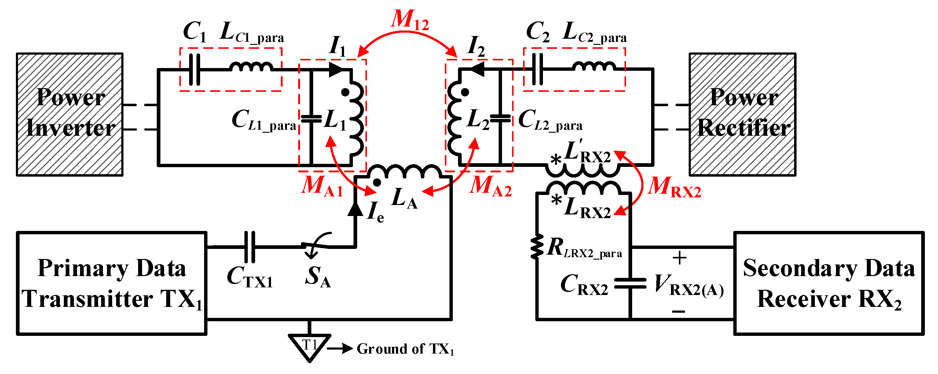
Figure 3 shows the positioning circuit model when S_A is switched on and the signal coil L_A is energized by TX₁. The circuit models for the other signal coils during working are the same. In Figure 3, both the power inverter on the primary side and the power rectifier on the secondary side can be seen as a short circuit for data carrier f_d1 due to their large DC bus capacitors. Three mutual inductances are formed between the primary power coil L₁, the secondary power coil L₂ and the energized signal coil L_A, respectively M₁₂, M_A1 and M_A2. The power resonant tank L₁C₁ and L₂C₂ are both resonant at the power frequency f_p (85 kHz). At the data carrier frequency f_d1 (5 MHz), the parasitic capacitances of the power inductors and the parasitic inductances of the power capacitors should be considered, which are denoted by C_{L1_para}, C_{L2_para}, L_{C1_para} and L_{C2_para}, respectively. Thus, the primary impedance Z₁ and the secondary impedance Z₂ at the data carrier frequency f_d1 can be derived as:

$$Z_1({\omega }_{\mathrm{d}1})=j{\omega }_{\mathrm{d}1}{L}_1+\frac{1-{\omega }_{\mathrm{d}1}^2{L}_{C1\_\mathrm{para}}{C}_1}{j{\omega }_{\mathrm{d}1}\left(C_1+C_{L1\_\mathrm{para}}-{\omega }_{\mathrm{d}1}^2{L}_{C1\_\mathrm{para}}{C}_1{C}_{L1\_\mathrm{para}}\right)},$$

(10)

$$Z_2({\omega }_{\mathrm{d}1})=j{\omega }_{\mathrm{d}1}{L}_2+\frac{Z_{\mathrm{branch}}}{1+j{\omega }_{\mathrm{d}1}{C}_{L2\_\mathrm{para}}{Z}_{\mathrm{branch}}}.$$

(11)

where

$$Z_{\mathrm{branch}}=\frac{1}{j{\omega }_{\mathrm{d}1}{C}_2}+j{\omega }_{\mathrm{d}1}{L}_{C2\_\mathrm{para}}+j{\omega }_{\mathrm{d}1}{L^{\prime }}_{\mathrm{RX}2}+\frac{{\omega }_{\mathrm{d}1}^2{M}_{\mathrm{RX}2}^2}{R_{L\mathrm{RX}2\_\mathrm{para}}}$$

Given that the current through L_A is I_e, the induced electromotive force (EMF) on the secondary power coil is:

$$\begin{array}{l}{\epsilon }_{2\left(\mathrm{A}\right)}({\omega }_{\mathrm{d}1})=j{\omega }_{\mathrm{d}1}{M}_{\mathrm{A}2}{I}_{\mathrm{e}}+j{\omega }_{\mathrm{d}1}{M}_{12}{I}_1\\ =j{\omega }_{\mathrm{d}1}\left(M_{\mathrm{A}2}-M_{12}\frac{{\omega }_{\mathrm{d}1}^2{M}_{12}{M}_{\mathrm{A}2}+j{\omega }_{\mathrm{d}1}{M}_{\mathrm{A}1}{Z}_2}{{\omega }_{\mathrm{d}1}^2{M}_{12}^2+Z_1{Z}_2}\right)I_{\mathrm{e}}\end{array}$$

(12)

The term in the parentheses of (12) can be defined as the effective mutual inductance M_eff(A) between the signal coil and the secondary coil, which synthesizes the reflection effect of the primary induced current I₁. The definition is:

$$M_{\mathrm{eff}\left(\mathrm{A}\right)}=M_{\mathrm{A}2}-M_{12}\frac{{\omega }_{\mathrm{d}1}^2{M}_{12}{M}_{\mathrm{A}2}+j{\omega }_{\mathrm{d}1}{M}_{\mathrm{A}1}{Z}_2}{{\omega }_{\mathrm{d}1}^2{M}_{12}^2+Z_1{Z}_2}.$$

(13)

Thus, the EMF on the secondary power coil when L_A is energized can be rewritten as:

$${\epsilon }_{2\left(\mathrm{A}\right)}({\omega }_{\mathrm{d}1})=j{\omega }_{\mathrm{d}1}{M}_{\mathrm{eff}\left(\mathrm{A}\right)}{I}_{\mathrm{e}}.$$

(14)

Since the four signal coils L_A–L_D are identical, the energized currents through them are same and equal to I_e. When L_A–L_D are energized in turns, the secondary induced EMF vector can be obtained as:

$$\left[\begin{array}{c}{\epsilon }_{2\left(\mathrm{A}\right)}\\ {\epsilon }_{2\left(\mathrm{B}\right)}\\ {\epsilon }_{2\left(\mathrm{C}\right)}\\ {\epsilon }_{2\left(\mathrm{D}\right)}\end{array}\right]=j{\omega }_{\mathrm{d}1}{I}_{\mathrm{e}}\cdot \left[\begin{array}{c}{M}_{\mathrm{eff}\left(\mathrm{A}\right)}\\ M_{\mathrm{eff}\left(\mathrm{B}\right)}\\ M_{\mathrm{eff}\left(\mathrm{C}\right)}\\ M_{\mathrm{eff}\left(\mathrm{D}\right)}\end{array}\right],$$

(15)

where the subscript A, B, C or D represents the coil L_A, L_B, L_C or L_D is energized, respectively.

Since the secondary signal extractor L_RX2 is fixed around the power line as shown in Figure 1a, the mutual inductance M_RX2 in Figure 3 is a constant. Meanwhile, in Figure 3, L_RX2 is resonant with C_RX2 at frequency ω_d1, and R_{LRX2_para} is the parasitic resistance of the signal extractor. Thus, the receiving amplitude |V_RX2| is proportional to the EMF on the secondary power coil, which can be derived as:

$$\left[\begin{array}{c}\left|V_{\mathrm{RX}2\left(\mathrm{A}\right)}\right|\\ \left|V_{\mathrm{RX}2\left(\mathrm{B}\right)}\right|\\ \left|V_{\mathrm{RX}2\left(\mathrm{C}\right)}\right|\\ \left|V_{\mathrm{RX}2\left(\mathrm{D}\right)}\right|\end{array}\right]=\left|\frac{{\omega }_{\mathrm{d}1}^2{M}_{\mathrm{RX}2}{L}_{\mathrm{RX}2}}{\left({\omega }_{\mathrm{d}1}^2{L}_2{C}_{L2\_\mathrm{para}}{Z}_{\mathrm{branch}}-Z_{\mathrm{branch}}-j{\omega }_{\mathrm{d}1}{L}_2\right)R_{L\mathrm{RX}2\_\mathrm{para}}}\right|\cdot \left[\begin{array}{c}\left|{\epsilon }_{2\left(\mathrm{A}\right)}\right|\\ \left|{\epsilon }_{2\left(\mathrm{B}\right)}\right|\\ \left|{\epsilon }_{2\left(\mathrm{C}\right)}\right|\\ \left|{\epsilon }_{2\left(\mathrm{D}\right)}\right|\end{array}\right].$$

(16)

Since four signal coils are fixed on the primary coil, the effective mutual inductance of each signal coil M_eff(A)–M_eff(D) is a function of the power coils’ relative position coordinate (x₁₂, y₁₂, z₁₂).

$$\left[\begin{array}{c}{M}_{\mathrm{eff}\left(\mathrm{A}\right)}\\ M_{\mathrm{eff}\left(\mathrm{B}\right)}\\ M_{\mathrm{eff}\left(\mathrm{C}\right)}\\ M_{\mathrm{eff}\left(\mathrm{D}\right)}\end{array}\right]=\left[\begin{array}{c}{F}_{\left(\mathrm{A}\right)}(x_{12},y_{12},z_{12})\\ F_{\left(\mathrm{B}\right)}(x_{12},y_{12},z_{12})\\ F_{\left(\mathrm{C}\right)}(x_{12},y_{12},z_{12})\\ F_{\left(\mathrm{D}\right)}(x_{12},y_{12},z_{12})\end{array}\right].$$

(17)

From (15)–(17), the relationship between the receiving signal amplitudes and the relative coordinate of power coils can be derived as:

$$\left[\begin{array}{c}\left|V_{\mathrm{RX}2\left(\mathrm{A}\right)}\right|\\ \left|V_{\mathrm{RX}2\left(\mathrm{B}\right)}\right|\\ \left|V_{\mathrm{RX}2\left(\mathrm{C}\right)}\right|\\ \left|V_{\mathrm{RX}2\left(\mathrm{D}\right)}\right|\end{array}\right]=\left|\frac{j{\omega }_{\mathrm{d}1}^3{M}_{\mathrm{RX}2}{L}_{\mathrm{RX}2}{I}_{\mathrm{e}}}{\left({\omega }_{\mathrm{d}1}^2{L}_2{C}_{L2\_\mathrm{para}}{Z}_{\mathrm{branch}}-Z_{\mathrm{branch}}-j{\omega }_{\mathrm{d}1}{L}_2\right)R_{L\mathrm{RX}2\_\mathrm{para}}}\right|\cdot \left[\begin{array}{c}{F}_{\left(\mathrm{A}\right)}(x_{12},y_{12},z_{12})\\ F_{\left(\mathrm{B}\right)}(x_{12},y_{12},z_{12})\\ F_{\left(\mathrm{C}\right)}(x_{12},y_{12},z_{12})\\ F_{\left(\mathrm{D}\right)}(x_{12},y_{12},z_{12})\end{array}\right].$$

(18)

The functions F_(A), F_(B), F_(C) and F_(D) in (18) can be derived from the Neumann formula (6), but they do not have the analytical expressions. Thus, Equation (18) cannot be used to directly calculate the relative coordinate from the receiving amplitudes. However, it confirms the one-to-one correspond-ence between the amplitude vector $\overrightarrow{V_{\mathrm{RX}2}}$(|V_RX2(A)|, |V_RX2(B)|, |V_RX2(C)|, |V_RX2(D)|) and the power coils’ relative coordinate $\overrightarrow{C_{12}}$(x₁₂, y₁₂, z₁₂). Thus, the lookup table method can be used to determine the position coordinate according to the amplitude vector.

3. Optimal Number and Locations for Auxiliary Signal Coils

According to (17) and (18), the change of the secondary coil position leads to the change of effective mutual inductances, and further leads to the change of receiving signal amplitudes. For the same position change, the more the effective mutual inductances change, the higher position resolution will be obtained, i.e., the higher positioning accuracy. Thus, the optimal locations for the signal coils are the places where the gradient of effective mutual inductance ∇M_eff is maximized.

$$\nabla M_{\mathrm{eff}}=\frac{\partial M_{\mathrm{eff}}}{\partial x}\overrightarrow{x}+\frac{\partial M_{\mathrm{eff}}}{\partial y}\overrightarrow{y}+\frac{\partial M_{\mathrm{eff}}}{\partial z}\overrightarrow{z}.$$

(19)

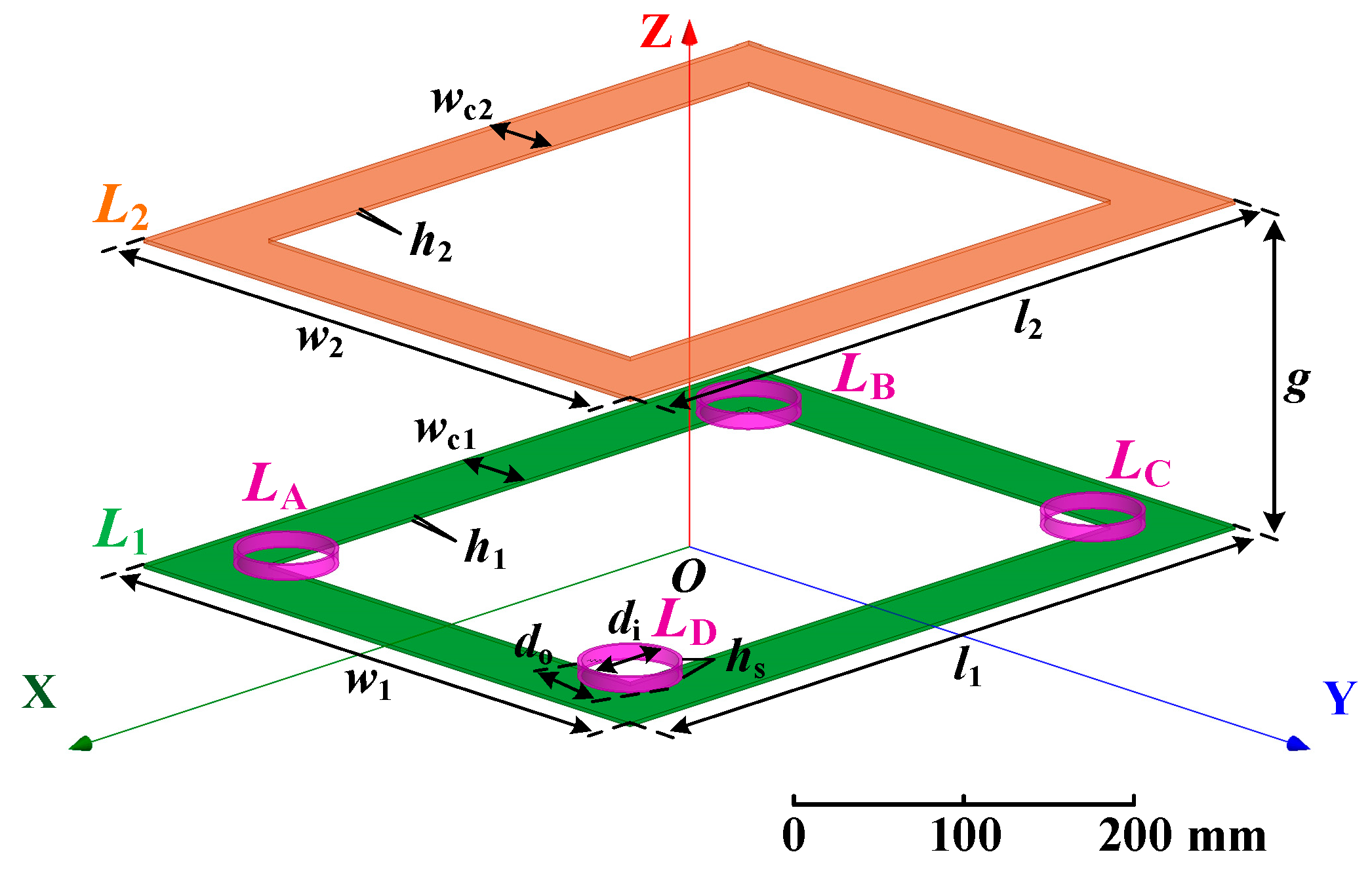
Simulations were conducted in ANSYS Electromagnetics Suite to find the optimal locations. The Cartesian coordinate system for positioning is built in Figure 4, of which the origin is set to the three-dimensional geometric center of the primary coil. The dimensions of the power coils and signal coils are listed in

Table 1. Coil dimensions.

Power Coils
Primary coil outer dimension l1 × w1 × h1	510 mm × 410 mm × 2.5 mm
Primary coil copper width wc1	52.5 mm
Secondary coil outer dimension l2 × w2 × h2	510 mm × 410 mm × 2.5 mm
Secondary coil copper width wc2	52.5 mm
Normal air gap g	160 mm
Auxiliary Signal Coils
Signal coil outer diameter do	63 mm
Signal coil inner diameter di	58 mm
Signal coil height hs	10 mm

. The position of each coil is represented by the coordinate of its three-dimensional geometric center. In the normal alignment condition, the primary coil coordinate (x₁, y₁, z₁) is (0, 0, 0), and the secondary coil coordinate (x₂, y₂, z₂) is (0, 0, 160 mm).

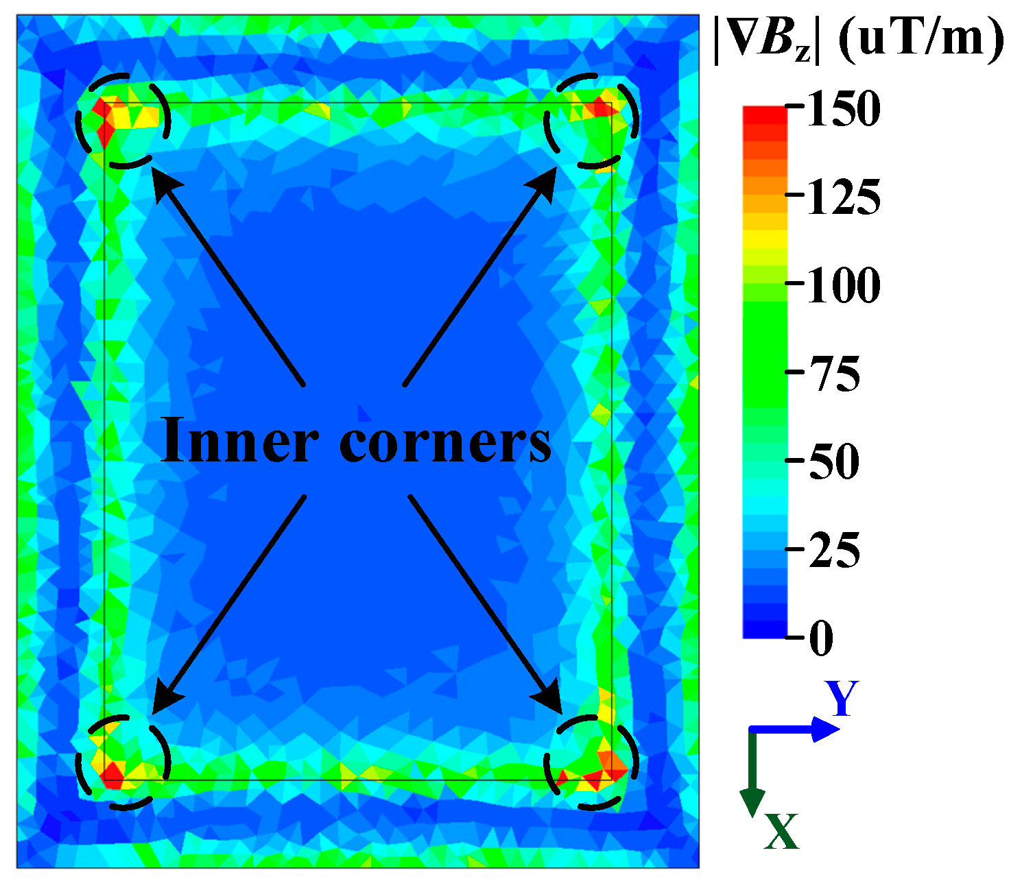
To minimize the installation space of the signal coils in practice, it is better to place the signal coils in parallel with the primary coil, i.e., in parallel with the XOY plane. In this condition, only the z-component of flux density through the signal coil will contribute to the effective mutual inductance with the secondary coil. Thus, we can energize the secondary coil and find the places where the gradient of flux density z-component ∇B_z is maximized. These places also have the maximized gradient of effective mutual inductance ∇M_eff. The gradient of flux density z-component ∇B_z is defined as:

$$\nabla B_{\mathrm{z}}=\frac{\partial B_{\mathrm{z}}}{\partial x}\overrightarrow{x}+\frac{\partial B_{\mathrm{z}}}{\partial y}\overrightarrow{y}+\frac{\partial B_{\mathrm{z}}}{\partial z}\overrightarrow{z}.$$

(20)

In the simulation, the secondary coil is energized with a 1-A current. Since the thickness of the signal coil is 10 mm, the gradient magnitude |∇B_z| on the plane 10 mm above the primary coil is depicted in Figure 5. It can be seen that the highest gradient magnitude appears at the four inner corners. This means the mutual inductance at these places will change to the greatest extent when the secondary coil position changes. Thus, the position resolution can be maximized when the signal coils are placed at the inner corners above the primary coil.

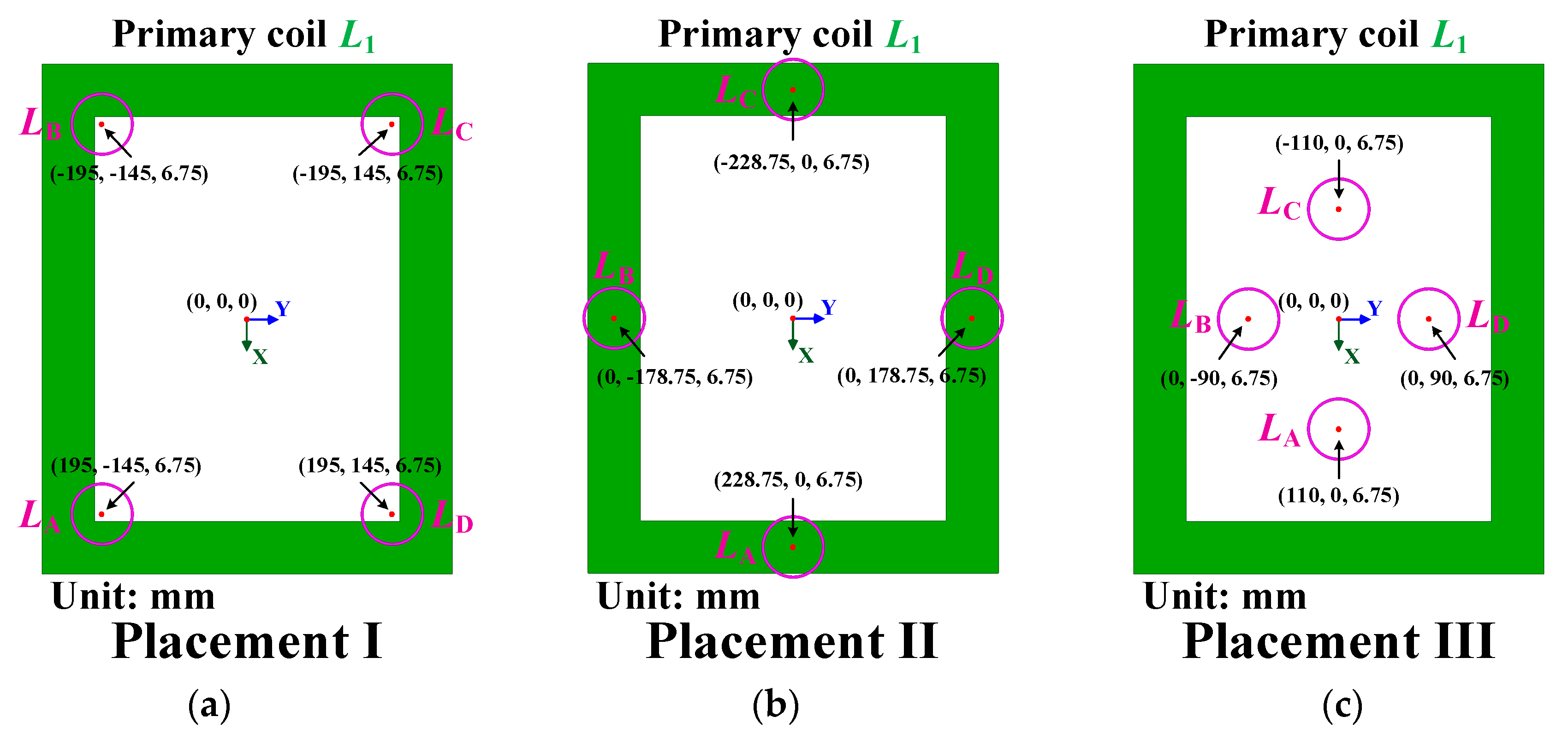
To verify the optimal locations for the signal coils, three kinds of signal coils placement are simulated and compared, as shown in Figure 6. The primary coil is colored by green, and the signal coils are colored by pink. Their coordinates are also given in Figure 6.

In the simulation, the primary coil coordinate (x₁, y₁, z₁) is always fixed at (0, 0, 0). In the initial condition, i.e., the normal alignment condition, the secondary coil coordinate (x₂, y₂, z₂) is (0, 0, 160 mm), which is also denoted by (x₂₀, y₂₀, z₂₀). Then the secondary coil moves along three axes, and its position change along three axes are denoted by Δx₂, Δy₂ and Δz₂, respectively.

$$(\Delta x_2,\Delta y_2,\Delta z_2)=(x_2-x_{20},y_2-y_{20},z_2-z_{20}),$$

(21)

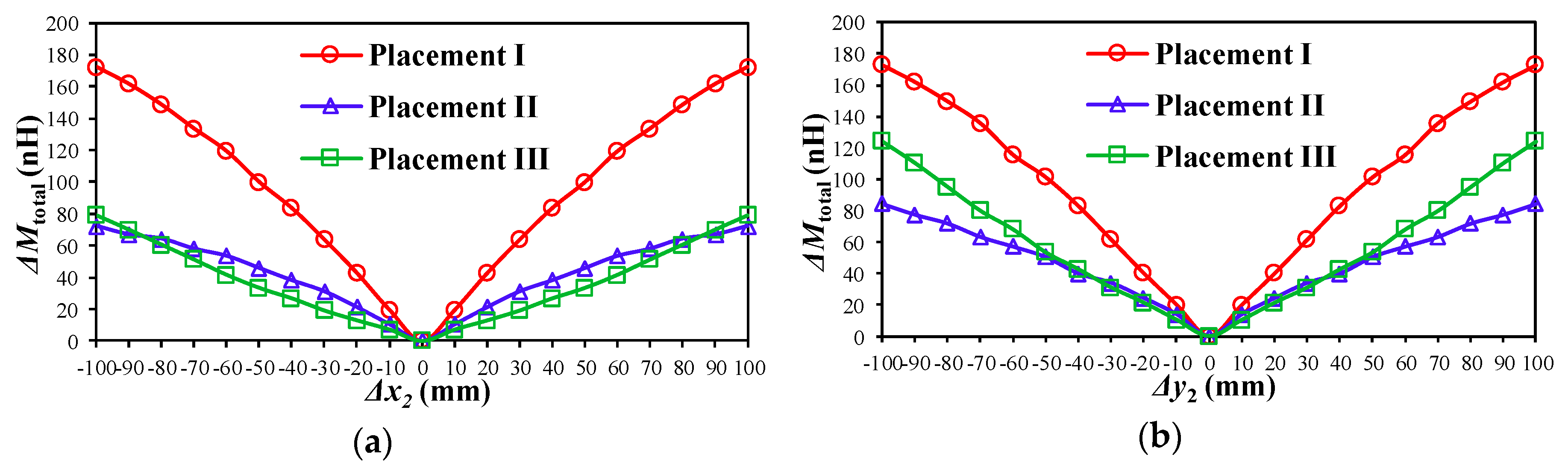
The total change of effective mutual inductances ΔM_total is used to evaluate the performance of coil placement, which is defined as:

$$\begin{array}{ll}\Delta M_{\mathrm{total}}& =\left|M_{\mathrm{eff}\left(\mathrm{A}\right)}-{M^{\prime }}_{\mathrm{eff}\left(\mathrm{A}\right)}\right|+\left|M_{\mathrm{eff}\left(\mathrm{B}\right)}-{M^{\prime }}_{\mathrm{eff}\left(\mathrm{B}\right)}\right|\\ & +\left|M_{\mathrm{eff}\left(\mathrm{C}\right)}-{M^{\prime }}_{\mathrm{eff}\left(\mathrm{C}\right)}\right|+\left|M_{\mathrm{eff}\left(\mathrm{D}\right)}-{M^{\prime }}_{\mathrm{eff}\left(\mathrm{D}\right)}\right|,\end{array}$$

(22)

where M’_eff(A), M’_eff(B), M’_eff(C), M’_eff(D) are the effective mutual inductances in the initial condition, i.e., when (x₂, y₂, z₂) is equal to (x₂₀, y₂₀, z₂₀), and M_eff(A), M_eff(B), M_eff(C), M_eff(D) are the effective mutual inductances when the secondary coil is moved. Thus, ΔM_total describes the total change of four effective mutual inductances relative to those of the initial position (x₂₀, y₂₀, z₂₀).

When the secondary coil moves along three axes, ΔM_total in the three placement conditions are depicted in Figure 7a–c. It can be seen that the Placement I always has the maximum ΔM_total for the same position change along x, y and z axes. The results are consistent with the gradient analysis in Figure 5. This means the Placement I will produce the maximum change of the receiving signal amplitude vector (|V_RX2(A)|, |V_RX2(B)|, |V_RX2(C)|, |V_RX2(D)|). As a result, the highest positioning resolution can be obtained from Placement I.

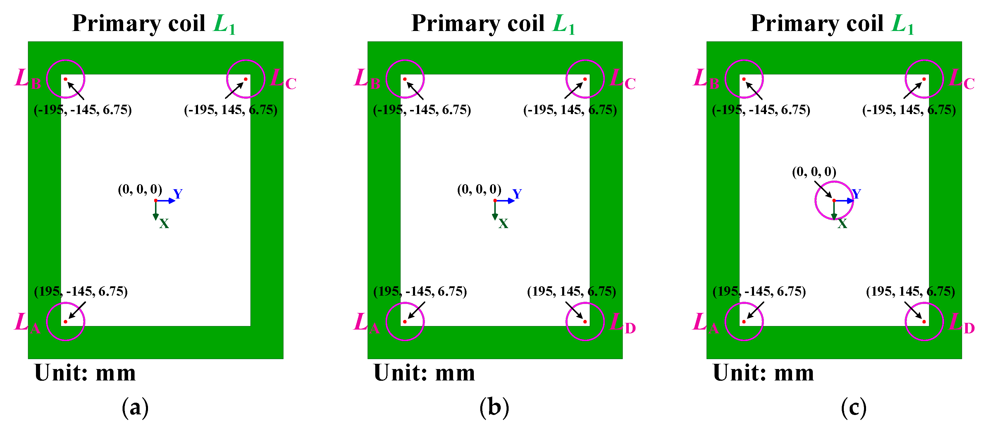
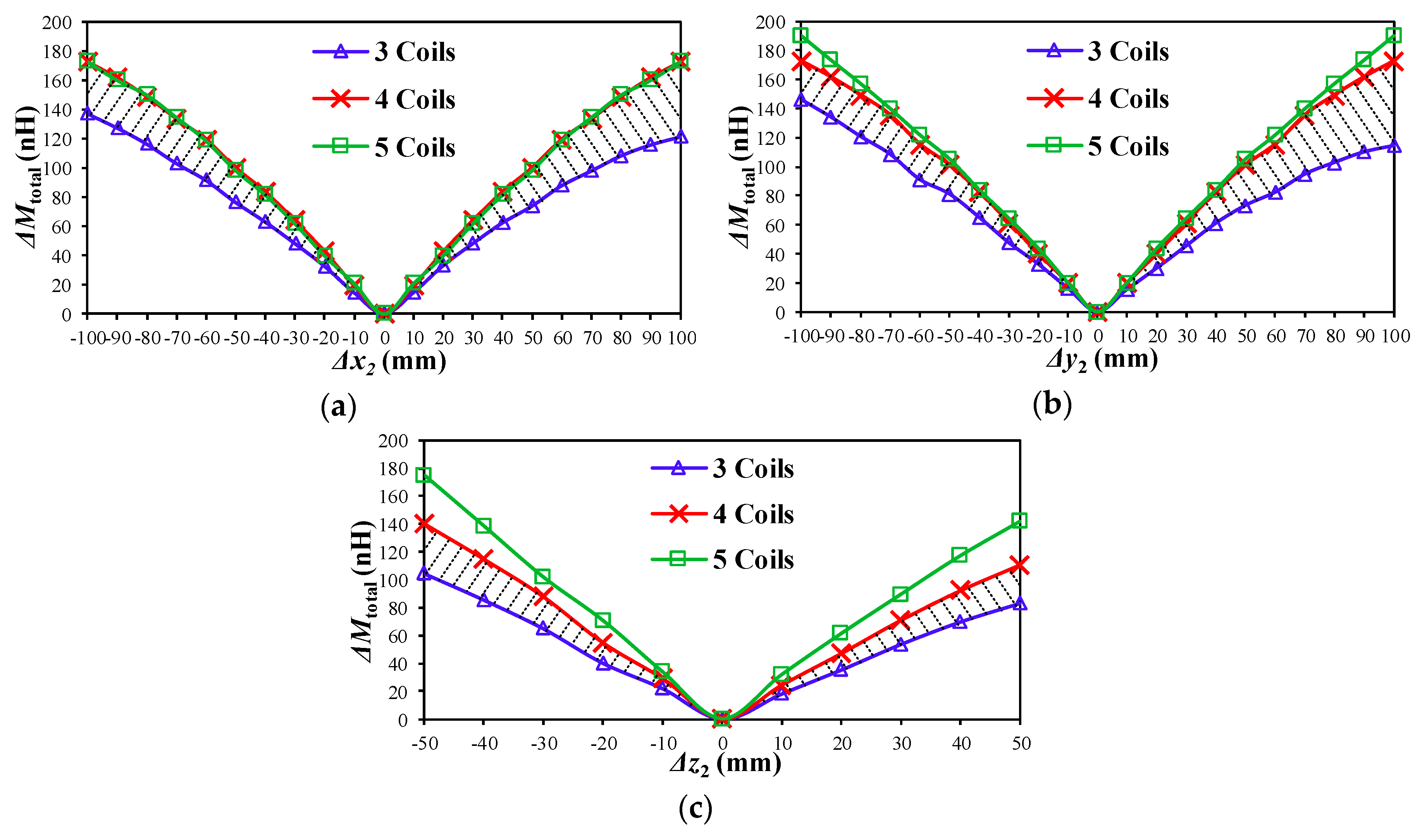
To find out the optimal number of signal coils, placements with different numbers of signal coils are analyzed. To achieve 3D positioning, at least three signal coils are needed. Thus, the placements with three coils, four coils and five coils are simulated, as shown in Figure 8. The placement with three coils occupies three inner corners to maximize the sensitivity, as shown in Figure 8a. The placement with four coils in Figure 8b is same as the Placement I in Figure 6a, which has been proved the best placement for the four-coil structure. The placement with five coils adds a central coil, as shown in Figure 8c. The results of ΔM_total for different numbers of coils are depicted in Figure 9a–c. Compared to three coils, four coils can significantly improve the position sensitivity in all three directions. These improvements are indicated by the shadow areas in Figure 9a–c. Specifically, ΔM_total is increased 42% at Δx = 100 mm, increased 51% at Δy = 100 mm, and increased 35% at Δz = −50 mm. However, from four coils to five coils, the further improvement is very limited. There are nearly no improvements in ΔM_total when moving along x and y axes. In the z direction, ΔM_total is increased only 25% at Δz = −50 mm. Thus, four coils are the most cost-effective with regard to accuracy and complexity. More than four coils bring little improvement in positioning accuracy but increase complexity and costs.

4. Amplitude Measurement of Positioning Signal

In Figure 3, the receiving positioning signal v_RX2 is a high-frequency sine wave (5 MHz). The conventional method to measure the amplitude is to rectify the high-frequency wave and sample the DC voltage by analog-to-digital converter (ADC) [33], i.e., the envelope detection. However, in the power transfer online condition, the envelope detector will be severely interfered by the power fundamental component, which is also received by signal extractor L_TX2. Thus, it is unsuitable for online positioning.

In [34], the data receiver circuit RX₂ has been proved immune to the power fundamental component when it works as data demodulator. Also, it is not hard to see that the data receiver output also contains the amplitude information of the receiving signal v_RX2, which is just neglected in the communication process in [34]. Thus, we can reuse the data receiver RX₂ to measure the positioning signal amplitude. No extra hardware is needed and the measurement is immune to the power fundamental interference.

The amplitude measurement circuit is separated from Figure 1a and redrawn in Figure 10a. Similar to (1) and (3), the transmitting signals v_LA–v_LD and the receiving signals v_RX2(A)–v_RX2(D) in positioning can be expressed as:

$$v_{Li}(t)=\left|V_{Li}\right|\sin \left(2\mathsf{\pi }{f}_{\mathrm{d}1}t+\phi (n)\right),$$

(23)

$$v_{\mathrm{RX}2(i)}(t)=\left|V_{\mathrm{RX}2(i)}\right|\sin \left(2\mathsf{\pi }{f}_{\mathrm{d}1}t+\phi (n)+{\phi }_{t(i)}\right),$$

(24)

where i = A, B, C or D, which indicates the transmitting coil. |V_Li| is the transmitting amplitude on L_A–L_D, |V_RX2(i)| is the receiving amplitude from L_A–L_D, and φ_t(i) is the phase shift of the transfer channel. φ(n) is the transmitting phase shift containing data bits, as illustrated in Section 2.1.

Since the receiving signals v_RX2(A)–v_RX2(D) are equivalent for the amplitude measurement circuit, the subscript i (i = A, B, C or D) is omitted in the following analysis for simplification. In Figure 10a, the receiving signal v_RX2 is divided by two identical resistors R_RX2 which are grounded at the center to produce a pair of differential outputs v_RX2+ and v_RX2−.

$$v_{\mathrm{RX}2+}=+\frac{v_{\mathrm{RX}2}}{2}=\frac{1}{2}\left|V_{\mathrm{RX}2}\right|\sin \left(2\mathsf{\pi }{f}_{\mathrm{d}1}t+\phi (n)+{\phi }_t\right),$$

(25)

$$v_{\mathrm{RX}2}{}_{-}=-\frac{v_{\mathrm{RX}2}}{2}=-\frac{1}{2}\left|V_{\mathrm{RX}2}\right|\sin \left(2\mathsf{\pi }{f}_{\mathrm{d}1}t+\phi (n)+{\phi }_t\right).$$

(26)

The differential signals v_RX2+ and v_RX2– are respectively connected to the two inputs, a and b, of the single-pole double-throw analog switches, S_cos2 and S_sin2. The output table of the analog switch is shown in

Table 2. Output table of analog switch.

Control Pin c	Output Pin o
High	Connected to input a
Low	Connected to input b

.

The control signals of two switches v_{c_sin2} and v_{c_cos2} are square waves with frequency f_d1’, and they are shifted by π/2 with each other, as shown in Figure 10b. Thus, each analog switch output v_{o_sin2} or v_{o_cos2} is equal to v_RX2+ multiplied by the respective square wave as:

$$\begin{array}{l}{v}_{\mathrm{o}\_\sin 2}=v_{\mathrm{RX}2+}\times \frac{4}{\mathsf{\pi }}{\displaystyle \sum _k\frac{\sin \left(k\cdot 2\mathsf{\pi }{f^{\prime }}_{\mathrm{d}1}t+k\cdot {\phi }_{\mathrm{c}}\right)}{k}}\\ =\frac{2\left|V_{\mathrm{RX}2}\right|}{\mathsf{\pi }}\sin \left(2\mathsf{\pi }{f}_{\mathrm{d}1}t+\phi (n)+{\phi }_t\right)\times {\displaystyle \sum _k\frac{\sin \left(k\cdot 2\mathsf{\pi }{f^{\prime }}_{\mathrm{d}1}t+k\cdot {\phi }_{\mathrm{c}}\right)}{k}}\end{array},$$

(27)

$$\begin{array}{l}{v}_{\mathrm{o}\_\cos 2}=v_{\mathrm{RX}2+}\times \frac{4}{\mathsf{\pi }}{\displaystyle \sum _k\frac{\cos \left(k\cdot 2\mathsf{\pi }{f^{\prime }}_{\mathrm{d}1}t+k\cdot {\phi }_{\mathrm{c}}\right)}{k}}\\ =\frac{2\left|V_{\mathrm{RX}2}\right|}{\mathsf{\pi }}\sin \left(2\mathsf{\pi }{f}_{\mathrm{d}1}t+\phi (n)+{\phi }_t\right)\times {\displaystyle \sum _k\frac{\cos \left(k\cdot 2\mathsf{\pi }{f^{\prime }}_{\mathrm{d}1}t+k\cdot {\phi }_{\mathrm{c}}\right)}{k}}\end{array}$$

(28)

where k = 1, 3, 5…; φ_c is the phase shift between the receiver control signal and the transmitter reference phase. In Figure 10b, φ_c and φ_t are both set to zero for clarity.

Applying the trigonometric product-to-sum formula to (27) and (28), it can be derived that v_{o_sin2} and v_{o_cos2} are composed of f_d1 ± kf_d1’ (k is odd) frequency components. If we set the control frequency f_d1’ equal to the data carrier frequency f_d1, v_{o_sin2} and v_{o_cos2} will have a DC component (i.e., f_d1 – f_d1’) and all the other components are higher than 2f_d1, as shown in Figure 10b. Since 2f_d1 ≫ 0, the DC components in v_{o_sin2} and v_{o_cos2} are easy to be obtained through low-pass filters (LPF), which are:

$$v_{\sin 2}(n)=\frac{\left|V_{\mathrm{RX}2}\right|}{\mathsf{\pi }}\cos \left(2\mathsf{\pi }(f_{\mathrm{d}1}-{f^{\prime }}_{\mathrm{d}1})t+\phi (n)+{\phi }_t-{\phi }_{\mathrm{c}}\right),$$

(29)

$$v_{\cos 2}(n)=\frac{\left|V_{\mathrm{RX}2}\right|}{\mathsf{\pi }}\sin \left(2\mathsf{\pi }(f_{\mathrm{d}1}-{f^{\prime }}_{\mathrm{d}1})t+\phi (n)+{\phi }_t-{\phi }_{\mathrm{c}}\right).$$

(30)

The DC voltages v_sin2(n) and v_cos2(n) are sampled by the digital signal processor (DSP). Then the amplitude of v_RX2 can be calculated by:

$$\left|V_{\mathrm{RX}2}\right|=\mathsf{\pi }\cdot \sqrt{v_{\sin 2}^2(n)+v_{\cos 2}^2(n)}.$$

(31)

It should be noted that if there is no PLL (phase-locked loop) in the receiver to synchronize the control signal frequency f_d1’ with the receiving positioning signal frequency f_d1, these two frequencies cannot be exactly equal. The results of (29) and (30) will be two very low-frequency (f_d1 – f_d1’) sine waves rather than two DC voltages, which is determined by the small deviation between f_d1 and f_d1’. However, this deviation will not affect the amplitude calculation, since (31) will eliminate the deviation frequency item 2π (f_d1 – f_d1’) t. Thus, the amplitude of high-frequency signal v_RX2 still can be determined by measuring these two very low-frequency sine waves. On the other hand, the receiving amplitude |V_RX2| is independent of the transmitting phase shift φ(n) which is related to data transmission. This means the position detection and the data transmission can work simultaneously through auxiliary coils L_A–L_D.

In the power transfer online condition, the power fundamental component interference f_p received on C_RX2 will be transformed to f_p ± kf_d1’ (k is odd) components at the outputs of analog switches according to (27) and (28). Since f_p << f_d1’, all the transformed components can be easily filtered out by LPF. Thus, the amplitude measurement is immune to the power fundamental component interference.

As discussed in Section 2, Equation (18) confirms the one-to-one correspondence between the amplitude vector $\overrightarrow{V_{\mathrm{RX}2}}$(|V_RX2(A)|, |V_RX2(B)|, |V_RX2(C)|, |V_RX2(D)|) and the power coils’ relative coordinate $\overrightarrow{C_{12}}$(x₁₂, y₁₂, z₁₂). Thus, the lookup table method can be used to determine the position coordinate $\overrightarrow{C_{12}}$(x₁₂, y₁₂, z₁₂) according to the measured amplitude vector $\overrightarrow{V_{\mathrm{RX}2}}$(|V_RX2(A)|, |V_RX2(B)|, |V_RX2(C)|, |V_RX2(D)|). The procedure of deriving the 3D position coordinate is illustrated by the flowchart in Figure 11.

5. Experimental Results

To verify the proposed magnetic positioning method, an experimental setup was built, as shown in Figure 12. The adopted data transceiver hardware is same as that proposed in [34]. Four auxiliary signal coils L_A–L_D are connected to the primary data transmitter TX₁ output through switches S_A–S_D, respectively. The positioning signal is extracted by L_RX2 and further processed by the secondary data receiver RX₂. The system parameters are listed in

Table 3. System parameters.

Power Transfer Circuit
Power carrier frequency fp	85 kHz
Power Coils L1 and L2 (uH)	85 and 85
Compensation capacitors C1 and C2 (nF)	45 and 42
Load resistor RL (Ω)	10
Primary Data Transmitter TX1
Forward data carrier frequency fd1	5 MHz
Input voltage Vd1	12 V
Auxiliary signal coils LA, LB, LC and LD	1.3 uH
CTX1	800 pF
Cs1	1000 pF
DC chokes Lf1	33 uH
MOSFET Q1	TPH3206LD
Power consumption	1.5 W
Secondary Data Receiver RX2
Signal extractors LRX2	1.4 uH
CRX2	700 pF
RRX2	15.1 kΩ
Analog switches Ssin2 and Scos2	TS5A23159
Corner frequency of LPF fc	35 kHz

.

The transmitting waveforms of four auxiliary signal coils are shown in Figure 13a, where v_LA–v_LD are the voltages on auxiliary signal coils L_A–L_D, respectively. It can be seen that L_A–L_D are enabled in turns to transmit positioning signals, and the enabled time is 1 s for each coil. The transmitting amplitudes of the four signal coils are equal, and keep constant during the power coils’ misalignment. There is a 20 ms dead time between two adjacent signal coils. Each signal coil sends its unique identity (ID) at 100 ms after being enabled, to tell the receiver which coil is sending the signal. The zoom-in waveforms in Figure 13b show the positioning signal is 5 MHz sine wave.

The receiving waveforms of secondary signal extractor L_RX2 is shown in Figure 14a. The signal extractor receives the positioning signal sent by L_A–L_D in turns. Since Figure 14a is measured without power coils’ misalignment, the voltage amplitudes received from L_A–L_D are nearly the same. The output of the amplitude measurement circuit is shown in Figure 14b. Since PLL is not adopted in the receiver, it can be seen that the waveforms of v_sin2 and v_cos2 are two very low-frequency sine waves (41 Hz) rather than two DC voltages due to the small deviation between f_d1 and f_d1’, as analyzed in Section 4. DSP samples these two very low-frequency sine waves, and the voltage amplitude received from each auxiliary signal coil |V_RX2(A)|–|V_RX2(D)| can be calculated according to (31).

The ID detection waveforms are shown in Figure 15. The DQPSK communication method is adopted, which has been illustrated in Section 2.1. The IDs for L_A–L_D are “A”–“D” in ASCII code, respectively. According to the data mapping table in Figure 2, the data transmitter TX₁ changes the signal phase to modulate the coil ID into the signal. In Figure 15, the phase change will result in the transient responses in both transmitter and receiver, which accounts for the voltage spikes in v_LA–v_LD and v_RX2 waveforms. The duration for each data symbol T_symbol is 31.25 us, and the bit rate is 64 kbps. On the receiver side, the phase changes are demodulated back to data, which are displayed by the high-bit pin and low-bit pin of DSP, as shown in Figure 15. The demodulation delay is 16 us.

When the secondary power coil position was changed, the receiving voltage waveforms v_RX2 were measured, as shown in Figure 16. In Figure 16a, the voltage amplitudes received from L_A–L_D are nearly equal when the secondary coil is aligned with the primary coil. This is because four signal coils are symmetric with respect to the secondary coil in this condition. In Figure 16b, the secondary coil was moved 100 mm along the x axis. The voltage amplitudes received from L_B and L_C are increased while the voltage amplitudes received from L_A and L_D are decreased. In Figure 16c, the secondary coil was moved 100 mm along the y axis. The voltage amplitudes received from L_A and L_B are increased while the voltage amplitudes received from L_C and L_D are decreased. In Figure 16d, the secondary coil was moved 50 mm along z axis. The voltage amplitudes received from L_A–L_D are nearly equal once again due to the symmetry. However, the receiving amplitudes in Figure 16d are smaller than those in Figure 16a because the effective mutual inductances between the auxiliary signal coils and the secondary power coil are reduced.

In the condition of 3.3 kW power transfer, the power interference to the positioning amplitude measurement was tested, as shown in Figure 17. In Figure 17a, the power inverter output voltage v_p and current i_p are shown in CH1 and CH2, respectively. The positioning transmitting waveform v_LA and receiving waveform v_RX2 are both superimposed with a 85 kHz component. Since the 85 kHz component received by L_RX2 is much larger than the 5 MHz component, the 5MHz component nearly cannot be identified in the receiving waveform v_RX2 in Figure 17a. However, in Figure 17b, it can be seen that the small 5 MHz component can still be extracted through the analog switches and LPF, and transformed to 41 Hz sine wave, i.e., v_sin2 and v_cos2. Meanwhile, the large 85 kHz power fundamental component has no effect on the waveforms of v_sin2 and v_cos2, which are sampled by DSP for amplitude calculation. Thus, the amplitude measurement is immune to the power fundamental interference, as analyzed in Section 4. The online positioning is achieved. It should be noted that the power losses caused by the signal coils during online positioning can be neglected, since the signal coils are resonant with the compensation capacitor C_TX1 at 5 MHz, which forms a bandpass filter to greatly suppress the power carrier of 85 kHz.

The measured voltage amplitudes when the secondary coil moves along x axis, y axis, z axis and the linear track y = x are shown in Figure 18a–d, respectively. The measurement is taken every 1-cm position change along x axis, y axis or z axis. The voltage amplitudes of |V_RX2(A)|–|V_RX2(D)| are represented by the digital values in DSP, which are calculated according to (31). The amplitude value at each position shown in Figure 18 is the average value of 20 repeated measurements. In the measurement, the maximum amplitude variation due to the background noise is 9 in digital value. Thus, the digital amplitude change less than 9 will be deemed as noise, and cannot be used to distinguish position. In Figure 18a, when Δx₂ ≥ 530 mm, the amplitude changes of |V_RX2(B)| and |V_RX2(C)| due to a 1-cm position change will be less than 9. When Δx₂ ≤ −530 mm, the amplitude changes of |V_RX2(A)| and |V_RX2(D)| due to 1-cm position change will be less than 9. In Figure 18b, when Δy₂ ≥ 450 mm, the amplitude changes of |V_RX2(A)| and |V_RX2(B)| due to a 1-cm position change will be less than 9. When Δy₂ ≤ −450 mm, the amplitude changes of |V_RX2(C)| and |V_RX2(D)| due to a 1-cm position change will be less than 9. According to the amplitude change rule mentioned above, a conservative positioning region in the normal air gap condition (g = 160 mm) can be derived as a 1060 mm × 900 mm elliptical region. Inside this region, the positioning resolution can keep no lower than 1 cm. The results of air gap changing conditions are shown in Figure 18c. The variation range of air gap is ± 100 mm. It can be seen that the positioning resolution along z axis can also keep no lower than 1 cm. Figure 18d shows the results when the secondary coil moves along the linear track y = x in the normal air gap condition. Since Δy₂ is always equal to Δx₂ on the line y = x, Figure 18d can be drawn in a two-dimensional plot, and Δx₂ is set as the horizontal axis. It can be seen that in the range |Δx₂| ≤ 350 mm, every 1-cm position change also can be distinguished.

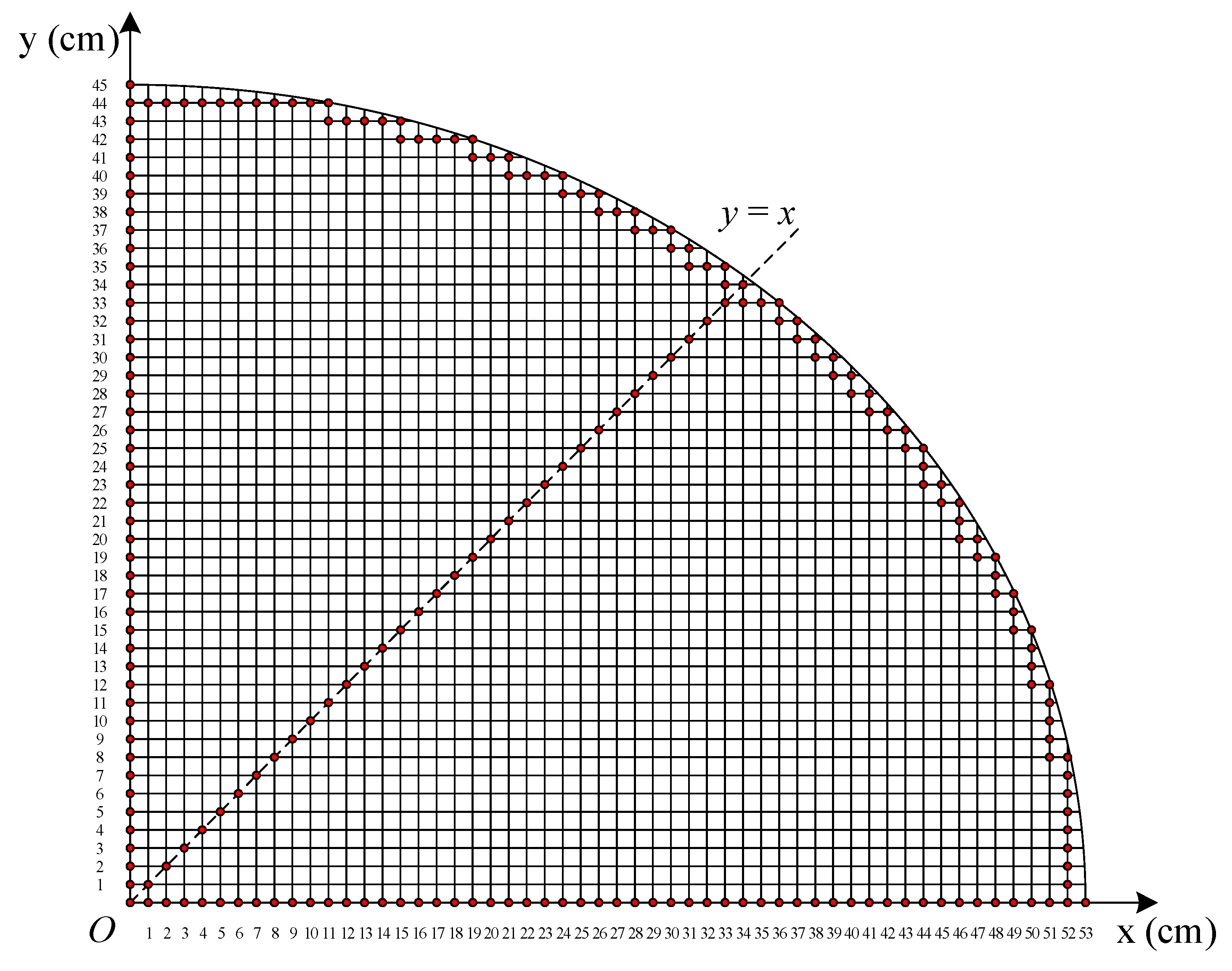
In the positioning experiment, the lookup table method was used to derive the real-time position coordinate according to the measured amplitude vector. The lookup table that links the amplitude vector $\overrightarrow{V_{\mathrm{RX}2}}$ (|V_RX2(A)|, |V_RX2(B)|, |V_RX2(C)|, |V_RX2(D)|) to the power coils’ relative coordinate $\overrightarrow{C_{12}}$(x₁₂, y₁₂, z₁₂) was established by the initial calibration. In the calibration, the amplitude vector $\overrightarrow{V_{\mathrm{RX}2}}$ was measured every 1-cm step along x, y and z axes in the whole positioning region, and then recorded together with the current coordinate $\overrightarrow{C_{12}}$. After calibration, 227 horizontal positions under three air gap conditions, respectively 110 mm, 160 mm and 210 mm, were tested to verify the positioning accuracy. The 227 horizontal positions are marked by red points in Figure 19, which include the positions on the outline of the quarter elliptical region and the positions on y = x. The minimum interval between these test points is 1 cm. Finally, all the coordinates of the total 681 test points were output accurately without error. The results show that the positioning accuracy of 1 cm is achieved.

6. Conclusions

In this paper, a magnetic positioning method based on the SWPDT system is proposed. A high integration of simultaneous power transfer, data transmission and position detection is achieved. The three-dimensional positioning accuracy achieves up to 1 cm. Compared to the conventional methods, the proposed positioning signal is transmitted by the auxiliary signal coils rather than the primary power coil. Thus, the operation of the primary high-power inverter will not be affected in the positioning process, and the online positioning can be achieved. The optimal locations for the auxiliary signal coils have been analyzed by finite element method (FEM) simulation, which are found to be the inner corners of the primary rectangular power coil. Since the signal coils for positioning are installed on the ground side, it can save the in-vehicle space and avoid the accuracy degrading due to the vehicle jolt. The amplitude measurement of the positioning signal is achieved by the data receiver circuit, which is immune to the power fundamental interference and ensures the online positioning accuracy. Moreover, all the communication needs in the positioning process can be satisfied well by SWPDT technology, and no extra RF communication hardware is needed.

References

- Galigekere, V.P.; Pries, J.; Onar, O.C.; Su, G.J.; Anwar, S.; Wiles, R.; Seiber, L.; Wilkins, J. Design and implementation of an optimized 100 kW stationary wireless charging system for EV battery recharging. In Proceedings of the 2018 IEEE Energy Conversion Congress and Exposition (ECCE), Portland, OR, USA, 23–27 September 2018. [Google Scholar]
- Li, W.; Zhao, H.; Deng, J.; Li, S.; Mi, C.C. Comparison study on SS and double-sided LCC compensation topologies for EV/PHEV wireless chargers. IEEE Trans. Veh. Technol. 2016, 65, 4429–4439. [Google Scholar] [CrossRef]
- Zhang, Z.; Pang, H.; Georgiadis, A.; Cecati, C. Wireless power transfer–an overview. IEEE Trans. Ind. Electron. 2019, 66, 1044–1058. [Google Scholar] [CrossRef]
- Budhia, M.; Covic, G.A.; Boys, J.T. Design and optimization of circular magnetic structures for lumped inductive power transfer systems. IEEE Trans. Power Electron. 2011, 26, 3096–3108. [Google Scholar] [CrossRef]
- Budhia, M.; Boys, J.T.; Covic, G.A.; Huang, C. Development of a single-sided flux magnetic coupler for electric vehicle IPT charging systems. IEEE Trans. Ind. Electron. 2013, 60, 318–328. [Google Scholar] [CrossRef]
- Zaheer, A.; Hao, H.; Covic, G.A.; Kacprzak, D. Investigation of multiple decoupled coil primary pad topologies in lumped IPT systems for interoperable electric vehicle charging. IEEE Trans. Power Electron. 2015, 30, 1937–1955. [Google Scholar] [CrossRef]
- Kim, S.; Covic, G.A.; Boys, J.T. Comparison of tripolar and circular pads for IPT charging systems. IEEE Trans. Power Electron. 2018, 33, 6093–6103. [Google Scholar] [CrossRef]
- Villa, J.L.; Sallan, J.; Sanz Osorio, J.F.; Llombart, A. High-misalignment tolerant compensation topology for ICPT systems. IEEE Trans. Ind. Electron. 2012, 59, 945–951. [Google Scholar] [CrossRef]
- Lu, F.; Zhang, H.; Hofmann, H.; Mi, C. A dual-coupled LCC-compensated IPT system to improve misalignment performance. In Proceedings of the IEEE PELS Workshop Emerging Technologies: Wireless Power Transfer (WoW), Chongqing, China, 20–22 May 2017. [Google Scholar]
- Zhao, L.; Thrimawithana, D.J.; Madawala, U.K. Hybrid bidirectional wireless EV charging system tolerant to pad misalignment. IEEE Trans. Ind. Electron. 2017, 64, 7079–7086. [Google Scholar] [CrossRef]
- Zhao, L.; Thrimawithana, D.J.; Madawala, U.K.; Hu, A.P.; Mi, C.C. A misalignment-tolerant series-hybrid wireless EV charging system with integrated magnetics. IEEE Trans. Power Electron. 2019, 34, 1276–1285. [Google Scholar] [CrossRef]
- Zhang, Z.; Krein, P.T.; Ma, H.; Tang, Y.; Zhou, J.; Xu, D. An inductive power transfer system design with large misalignment tolerance for EV charging. In Proceedings of the IEEE 27th International Symposium on Industrial Electronics, Cairns, Australia, 13–15 June 2018. [Google Scholar]
- Wireless Power Transfer for Light-Duty Plug-in/Electric Vehicles and Alignment Methodology, SAE J2954 Recommended Practice. 2017. Available online: https://www.sae.org/standards/content/j2954_201605/ (accessed on 26 February 2020).
- Chen, S.; Liao, C.; Wang, L. Research on positioning technique of wireless power transfer system for electric vehicles. In Proceedings of the IEEE Conference and Expo Transportation Electrification Asia-Pacific (ITEC Asia-Pacific), Beijing, China, 31 August–3 September 2014. [Google Scholar]
- Tiemann, J.; Pillmann, J.; Bocker, S.; Wietfeld, C. Ultra-wideband aided precision parking for wireless power transfer to electric vehicles in real life scenarios. In Proceedings of the IEEE 84th Vehicular Technology Conference (VTC-Fall), Montreal, QC, Canada, 18–21 September 2016. [Google Scholar]
- Ni, L.M.; Liu, Y.; Lau, Y.C.; Patil, A.P. LANDMARC: Indoor location sensing using active RFID. In Proceedings of the First IEEE International Conference on Pervasive Computing and Communications 2003 (PerCom 2003), Fort Worth, TX, USA, 26 March 2003. [Google Scholar]
- Bouet, M.; dos Santos, A.L. RFID tags: Positioning principles and localization techniques. In Proceedings of the 2008 1st IFIP Wireless Days, Dubai, UAE, 24–27 November 2008. [Google Scholar]
- Xu, H.; Ding, Y.; Li, P.; Wang, R.; Li, Y. An RFID indoor positioning algorithm based on Bayesian probability and K-Nearest Neighbor. Sensors 2017, 17, 1806. [Google Scholar] [CrossRef] [Green Version]
- Xu, H.; Wu, M.; Li, P.; Zhu, F.; Wang, R. An RFID indoor positioning algorithm based on support vector regression. Sensors 2018, 18, 1504. [Google Scholar] [CrossRef] [PubMed] [Green Version]
- Lee, K.; Kim, J.; Cha, C. Microwave-based wireless power transfer using beam scanning for wireless sensors. In Proceedings of the IEEE EUROCON 2019-18th International Conference on Smart Technologies, Novi Sad, Serbia, 1–4 July 2019. [Google Scholar]
- Liu, L.; Niu, P.; Luo, D.; Guo, Y.; Sun, Y. A method for aligning of transmitting and receiving coils of electric vehicle wireless charging based on binocular vision. In Proceedings of the 2017 IEEE Conference on Energy Internet and Energy System Integration (EI2), Beijing, China, 26–28 November 2017. [Google Scholar]
- Shieh, W.; Hsu, C.J.; Wang, T. Vehicle positioning and trajectory tracking by infrared signal-direction discrimination for short-range vehicle-to-infrastructure communication systems. IEEE Trans. Intell. Transp. Syst. 2018, 19, 368–379. [Google Scholar] [CrossRef]
- Langer, D.; Thorpe, C. Sonar based outdoor vehicle navigation and collision avoidance. In Proceedings of the IEEE/RSJ International Conference on Intelligent Robots and Systems, Raleigh, NC, USA, 7–10 July 1992. [Google Scholar]
- Han, W.; Chau, K.T.; Jiang, C.; Liu, W. Accurate position detection in wireless power transfer using magnetoresistive sensors for implant applications. IEEE Trans. Magn. 2018, 54, 4001205. [Google Scholar] [CrossRef]
- Liu, X.; Han, W.; Liu, C.; Pong, P.W.T. Marker-free coil-misalignment detection approach using TMR sensor array for dynamic wireless charging of electric vehicles. IEEE Trans. Magn. 2018, 54, 4002305. [Google Scholar] [CrossRef]
- Liu, X.; Liu, C.; Han, W.; Pong, P.W.T. Design and implementation of a multi-purpose TMR sensor matrix for wireless electric vehicle charging. IEEE Sens. J. 2019, 19, 1683–1692. [Google Scholar] [CrossRef]
- Liu, X.; Liu, C.; Pong, P.W.T. TMR-sensor-array-based misalignment-tolerant wireless charging technique for roadway electric vehicles. IEEE Trans. Magn. 2019, 55, 4003107. [Google Scholar] [CrossRef]
- Hwang, K.; Park, J.; Kim, D.; Park, H.H.; Kwon, J.H.; Kwak, S.I.; Ahn, S. Autonomous coil alignment system using fuzzy steering control for electric vehicles with dynamic wireless charging. Math. Probl. Eng. 2015, 2015, 205285. [Google Scholar] [CrossRef] [Green Version]
- Hwang, K.; Cho, J.; Kim, D.; Park, J.; Kwon, J.H.; Kwak, S.I.; Park, H.H.; Ahn, S. An autonomous coil alignment system for the dynamic wireless charging of electric vehicles to minimize lateral misalignment. Energies 2017, 10, 315. [Google Scholar] [CrossRef]
- Cortes, I.; Kim, W. Lateral position error reduction using misalignment-sensing coils in inductive power transfer systems. IEEE ASME Trans. Mechatron. 2018, 23, 875–882. [Google Scholar] [CrossRef]
- Moghaddami, M.; Sundararajan, A.; Sarwat, A.I. Sensorless electric vehicle detection in inductive charging stations using self-tuning controllers. In Proceedings of the IEEE Transportation Electrification Conference (ITEC-India), Pune, India, 13–15 December 2017. [Google Scholar]
- Gao, Y.; Duan, C.; Oliveira, A.A.; Ginart, A.; Farley, K.B.; Tse, Z.T.H. 3-D coil positioning based on magnetic sensing for wireless EV charging. IEEE Trans. Transp. Electrif. 2017, 3, 578–588. [Google Scholar] [CrossRef]
- Jeong, S.Y.; Kwak, H.G.; Jang, G.C.; Choi, S.Y.; Rim, C.T. Dual-purpose nonoverlapping coil sets as metal object and vehicle position detections for wireless stationary EV chargers. IEEE Trans. Power Electron. 2018, 33, 7387–7397. [Google Scholar] [CrossRef]
- Qian, Z.; Yan, R.; Wu, J.; He, X. Full-duplex high-speed simultaneous communication technology for wireless EV charging. IEEE Trans. Power Electron. 2019, 34, 9369–9373. [Google Scholar] [CrossRef]
- Yan, R.; Qian, Z.; Wu, J.; He, X. Magnetic coupling positioning using simultaneous power and data transfer. In Proceedings of the 44th Annual Conference of IEEE Industrial Electronics Society, Washington, DC, USA, 21–23 October 2018. [Google Scholar]
Figure 1.
Simultaneous wireless power and data transmission (SWPDT) system: (a) original communication setting; (b) proposed positioning setting.
Figure 2.
Differential quadrature phase-shift keying (DQPSK) modulation of data transmitter.
Figure 3.
Positioning circuit model when LA is energized.
Figure 4.
Coordinate system for positioning.
Figure 5.
Distribution of the gradient magnitude |∇Bz| on the plane 10 mm above the primary coil.
Figure 6.
Three placements of auxiliary signal coils: (a) placed above four inner corners of the primary coil; (b) placed above four sides’ midpoints of the primary coil; (c) placed above the primary coil interior.
Figure 7.
Total change of effective mutual inductances ΔMtotal when the secondary coil moves along: (a) x axis; (b) y axis; and (c) z axis.
Figure 8.
Placement with different coil number: (a) three signal coils; (b) four signal coils; (c) five signal coils.
Figure 9.
ΔMtotal obtained by different numbers of signal coils when the secondary coil moves along: (a) x axis; (b) y axis; and (c) z axis.
Figure 10.
Amplitude measurement: (a) circuit; (b) waveforms.
Figure 11.
Procedure for deriving 3D position coordinate.
Figure 12.
Experimental setup of proposed magnetic positioning method.
Figure 13.
(a) Transmitting waveforms of auxiliary signal coils; (b) zoom-in waveforms when LC is enabled.
Figure 14.
(a) Receiving waveforms of secondary signal extractor LRX2; (b) amplitude measurement waveforms when LA is enabled.
Figure 15.
Identity (ID) detection waveforms of auxiliary signal coils: (a) LA; (b) LB; (c) LC; and (d) LD.
Figure 16.
Receiving voltage waveforms when the position change of secondary power coil (Δx2, Δy2, Δz2) is equal to: (a) (0, 0, 0) mm; (b) (100, 0, 0) mm; (c) (0, 100, 0) mm; and (d) (0, 0, 50) mm.
Figure 17.
Online positioning under 3.3 kW power transfer: (a) transmitting waveform vLA and receiving waveform vRX2; (b) amplitude measurement waveforms vsin2 and vcos2.
Figure 18.
Measured receiving voltage amplitude when the position of secondary power coil changes along: (a) x axis; (b) y axis; (c) z axis; and (d) the line y = x in the normal air gap condition.
Figure 19.
Horizontal positions for positioning accuracy verification.