Development and Experimental Validation of a Supercapacitor Frequency Domain Model for Industrial Energy Applications Considering Dynamic Behaviour at High Frequencies

Abstract

Supercapacitors, one of the most promising energy storage technologies for high power density industrial applications, exchange the energy mostly through power electronic converters, operating under high frequency components due to the commutation. The high frequency produces important effects on the performance of the supercapacitors in relation to their capacitance, inductance and internal resistance (ESR). These parameters are fundamental to evaluate the efficiency of this energy storage system. The aim of the paper is to obtain an accurate model of two supercapacitors connected in series (functional and extrapolated unit) to represent the frequency effects for a wide range of frequencies. The methodology is based on the definition of an appropriate equivalent electric circuit with voltage dependance, obtaining their parameters from experimental tests, carried out by means of electrochemical impedance spectroscopy (EIS) and the use of specific software tools such as EC-Lab^® and Statgraphics Centurion^®. The paper concludes with a model which reproduces with accuracy both the frequency response of the model BCAP3000 supercapacitors, provided by the manufacturer, and the experimental results obtained by the authors.

1. Introduction

Among the variety of energy storage systems available for industrial applications, supercapacitors (SCs) have emerged as one of the most selected solutions when high power density, high efficiency, long lifespan, and extended range of operating temperatures are required. Specifically, SCs are widely employed in industry fields where there is a need for storing or releasing a relatively low amount of energy in a very short time and large number of charge-discharge cycles [1,2].

Although SCs are used in many applications by themselves for peak-power pulses reduction or compensation of power oscillations, they can also be hybridized with other energy storage systems, thus increasing the performance of the combined system. Transportation, uninterruptible power supply (UPS), and energy harvesting are the most relevant applications. Firstly, SCs are used in automotive industry to increase the efficiency of hybrid electric vehicles, either for an efficient restart of the engine after a stop, either for limiting the battery current peaks and improving the regenerative breaking in batteries-SCs hybrid vehicles, or for enhancing the dynamic response and load levelling in case of fuel cell-SCs hybrid vehicles [3,4,5,6,7]. Secondly, the UPS industry employs hybrid batteries-SCs systems for reducing the battery stress and extending the lifespan of the system. Moreover, in applications where long-time backups are not required, SCs can totally replace the battery storage system [8,9,10]. Thirdly, SCs are used in the energy harvesting industry for their integration with non-dispatchable renewable energy sources, i.e., wind and solar energies. The intermittent nature and uncertain prediction of these energy resources results in voltage and frequency fluctuations, which can destabilise the electric grid. Hence, energy storage systems, particularly SCs, play an important role in frequency regulation and peak shaving [11,12,13].

SCs modelling has become of maximum importance when designing and dimensioning SC installations since it is the way to know in advance about the behaviour and performance of the energy storage system when applied to particular operation profiles or conditions. Control strategies or operational parameters and limits can also be obtained from a model, enlarging the lifetime of the storage technology and therefore achieving a higher level of reliability and competitiveness. Numerous SC models have been published in the literature for different purposes, including capturing electrical dynamic behaviour, which is of utmost importance for the aforementioned industrial applications. The models that capture electrical behaviour of SCs can be classified in three main categories: electrochemical models, intelligent models and equivalent circuit models [2].

Commonly, electrochemical models account for high accuracy and low calculation efficiency, since they capture the reactions inside the SCs by employing coupled partial differential equations (PDEs). Among the electrochemical models, the three-domain model based on the uniform formulation of electrode-electrolyte system developed by Allu et al., and the three-dimensional (3D) model for SCs that considers 3D electrode morphology developed by Wang and Pilon are the most relevant [14,15].

Intelligent modelling techniques, such as artificial neural network (ANN) and fuzzy logic, have the capability of depicting the nonlinear relationship between the performance and its influencing factors, without a detailed understanding of the reactions inside the SCs. Nevertheless, a large amount of training data is needed to ensure model accuracy and generality. The most relevant models in this category are the established ANN model developed by Wu et al., and the one-layer feed-forward ANN developed by Eddahech et al. [16,17].

Equivalent circuit models mimic the electrical behaviour of SCs with parametrised capacitors, inductances, and resistors (RLC). They aim for simplicity, substituting PDEs with ordinary differential equations (ODEs), which hugely facilitate their implementation and make them particularly suitable for industry application analysis and studies. Their accuracy varies depending on the complexity, i.e., number of elements and circuit configuration. In the majority of cases, higher complexity implies higher accuracy.

Three subcategories can be considered for equivalent circuit models: RC models, transmission line models, and dynamic models. The latter, commonly referred to as frequency domain models, account for the best overall performance in terms of complexity, accuracy, and robustness [18]. In this sense, Buller et al. proposed an SC model using electrochemical impedance spectroscopy (EIS) in the frequency domain, with only four experimental parameters [19]. Moreover, Rafik et al. presented a frequency domain model with 14 RLC elements whose values are functions of voltage and/or temperature estimated through EIS methodology [20]. At last, Lajnef et al. developed a less complex frequency domain model for representing the dynamic behaviour of SCs, concluding that SCs present a behaviour which is capacitive at low frequencies, equivalent to a transmission line at intermediate frequencies, and inductive at high frequencies [21].

This paper proposes a new frequency-domain electric model for SCs which considers parameter variations with voltage and self-discharge behaviour. The model improves the overall accuracy of previous frequency-domain models, especially for high frequencies, while keeping a similar degree of complexity and calculation efficiency. A model validation is performed with experimental data collected in the authors’ laboratory through EIS tests. The paper is organized as follows: Section 2 presents a review of the most relevant frequency-domain models of SCs. The main contributions of the proposed SC model and its relevance for industry are also highlighted in Section 2. Section 3 describes the experimental tests performed for characterising the SCs behaviour as a function of frequency and voltage, together with the obtained results. The adjustment and description of the SC model is performed in Section 4, together with the comparison between the developed electric model and the collected experimental data. At last, conclusions are discussed in Section 5.

2. Review of the Existing Models of Supercapacitors in the Frequency Domain

When developing a new model that improves one or more features of the existent ones, a comprehensive review of the state of the art is needed. As mentioned in Section 1, the most relevant frequency-domain models reported in the literature are those of Buller et al., Rafik et al., and Lajnef et al. [19,20,21]. Buller et al. proposed an SC dynamic model using EIS in the frequency domain, which is depicted in Figure 1. The real part of the complex impedance (${\underset{\_}{Z}}_p$), which represents the porosity of the SC electrodes, increases as the frequency decreases, so the full SC capacitance is only available for DC conditions. Besides, a constant $L$ is included for representing the SC behavior at high frequencies in a simple way, while $R_i$ represents the series internal resistance.

The main contribution of this model is the huge reduction in the number of parameters that need to be determined, diminishing this number to four: $L$, $R_i$, $C$, and the capacitor charge time constant $\tau$ (needed to calculate $R_n$). Moreover, the model takes into account parameter dependency with temperature and voltage, producing precise results. As a counterpart, this dependency requires a large number of EIS measurements, which is time demanding. Moreover, these results are fed into lookup tables, which makes the model non-generalizable and hard to parametrise. Furthermore, the model lacks versatility, since it cannot be used for non-dynamic applications due to the absence of self-discharge modelling. At last, high frequency behaviour is simplified with a constant $L$, which results in an inaccurate behaviour for frequencies higher than $1\mathrm{kHz}$.

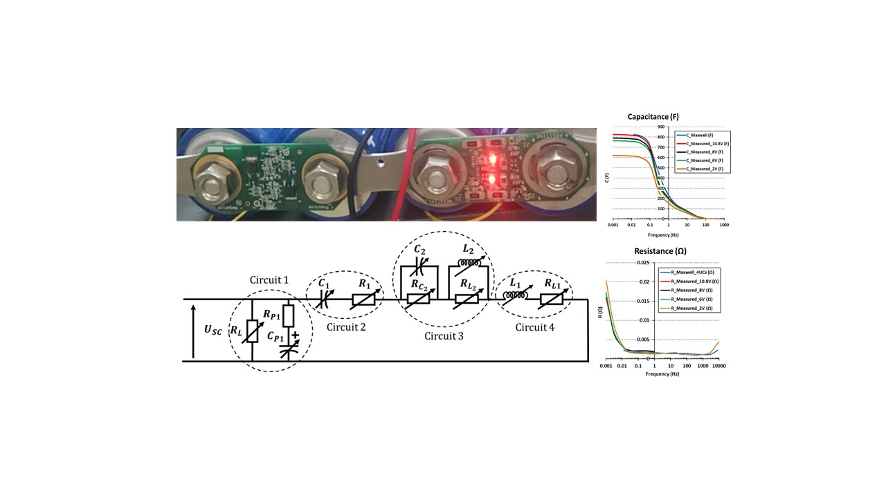
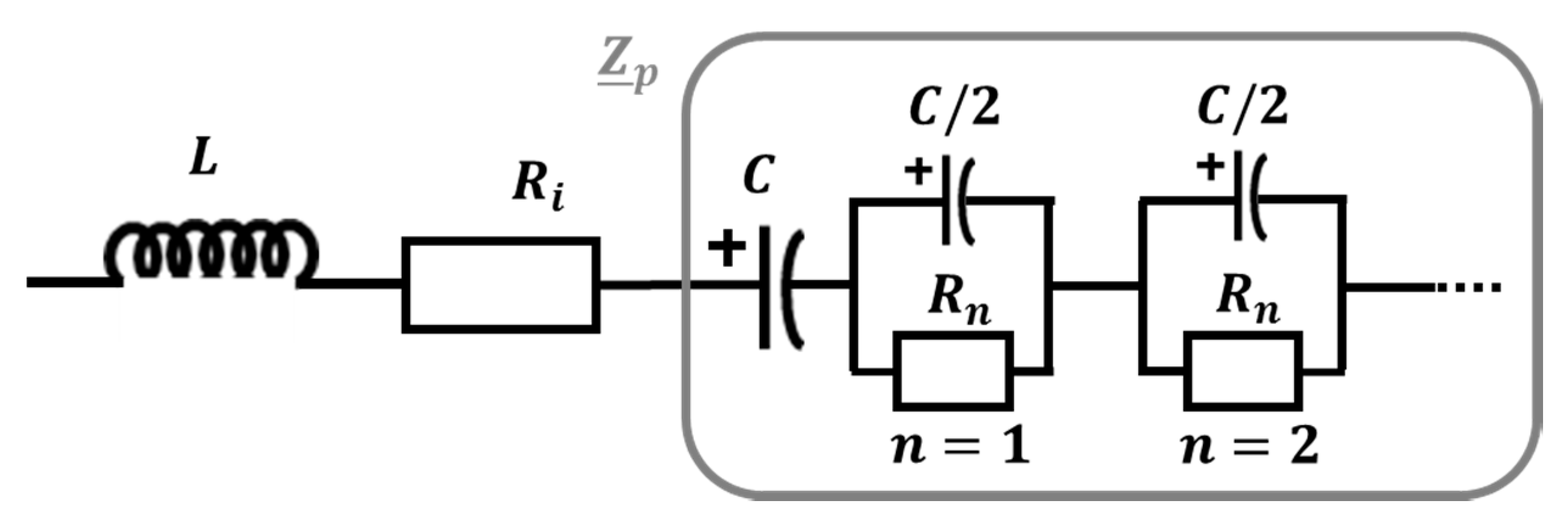
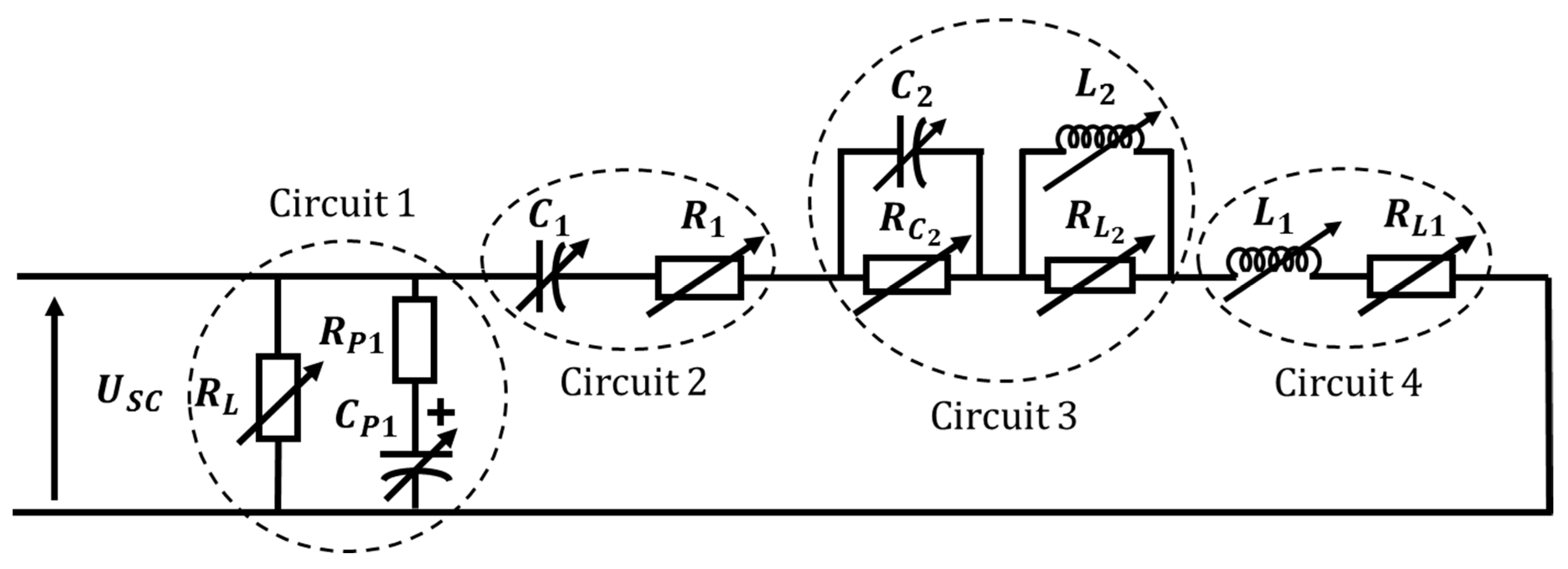
The SC model developed by Rafik et al. follows a similar methodology as Buller et al. Parameters are frequency, temperature, and voltage dependent, and are determined from experimental data using EIS. The model is shown in Figure 2.

The SC behaviour is represented by 14 parameters, being $L$ the equivalent inductance for high frequency ranges, $R_e$ the electronic resistance due to all connections, and $C_a$ the principal capacitance. Circuit 1, compounded by $R_V$ and $C_V$, models the voltage behaviour at low frequencies, while Circuit 2 takes into account the temperature dependency of the electrolyte ionic resistance in the low frequency range. Circuit 3 is introduced in the model to increase the value of the principal capacitance for average frequencies. Finally, Circuit 4 describes the leakage current and the internal charge redistribution, i.e., the self-discharge behaviour of the SC which is also temperature dependent.

The main contribution of the model proposed by Rafik et al. is the detailed behaviour modelling achieved through the inclusion of 3 correction circuits. Furthermore, the model takes into account the leakage current and the charge redistribution on the electrode, making it versatile for a great variety of studies. Moreover, the model is analytical (no lookup tables are required), which makes the model easily generalizable. The main drawback of this model is the huge number of EIS tests that are required to determine the parameters, which is time demanding. Moreover, frequencies higher than $1\mathrm{kHz}$, the behaviour is simplified through a constant $L$ value, which outcomes unprecise results.

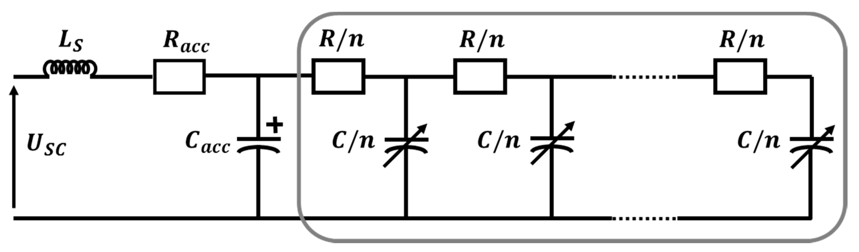
The frequency domain model developed by Lajnef et al. considers the SC behaviour as a function of frequency and voltage, without considering temperature dependency. Experimental data to model the SC behaviour has also been obtained through EIS tests. The model is displayed in Figure 3.

The SC is represented by a serial inductor ($L_s$), an access resistor which physically corresponds to the resistance of the device terminals ($R_{acc}$), a capacitor ($C_{acc}$), and a non-linear transmission line with voltage-dependent capacitors. The model considers some simplifications in order to be non-complicated and suitable for frequencies in the range from $10\mathrm{mHz}$ to $1\mathrm{kHz}$: charge redistribution and self-discharge is neglected, high frequency behaviour is not modelled, the impedance real-part dependency on voltage is neglected, and the transmission line is approached by a number of $N\mathrm{RC}$ branches. The higher the order $N$, the better the dynamic response is reproduced by the model.

The main contribution of this model is its simplicity, while keeping a reasonable accuracy for frequencies from $10\mathrm{mHz}$ to $1\mathrm{kHz}$. In addition, the number of EIS tests to perform is low when compared to other models, and the model can be easily parametrized. Furthermore, the model is analytical (no lookup tables are required). As a counterpart, not taking into account temperature and self-discharge effects limits its applicability. At last, SC behaviour for high frequencies is not modelled, making the model non-valid for frequencies higher than $1\mathrm{kHz}$.

Considering the drawbacks of the reviewed models, neither of them model the SC behaviour at high frequencies. Although charge/discharge frequency of SCs in industrial applications is usually lower than 1 kHz, high frequency components are always present due to the fact that SCs are integrated with the application by means of power electronic converters. The commutation frequency is in the range of $5$ to $50\mathrm{kHz}$ for IGBT modules, and higher to $100\mathrm{kHz}$ for MOSFET modules [22]. Besides, industry tends to increase this switching frequency with technologies like silicon carbide. This high-frequency components of voltage and current supplied by the power converter are neglected by the models reported in the literature. Hence, in order to develop a SC model that is suitable for the industry, the high-frequency behaviour of SCs needs to be taken into account.

The model developed in this paper, described in detail in Section 4, takes into account the high-frequency behaviour of a SC, which improves the accuracy for switching frequencies higher than $1\mathrm{kHz}$. Moreover, the model is analytical (no lookup tables are required), and has a low number of parameters, which simplifies the parametrisation process and makes it generalizable. The model considers voltage dependence of all parameters, but it does not take into account temperature effects, since, as stated by manufacturers, for temperatures higher than 20 °C, SC properties remain almost constant [23]. This consideration limits its applicability to low temperatures. However, it simplifies the model without compromising the accuracy for operating temperatures from 20 °C to 65 °C. Finally, the developed model includes charge redistribution and self-discharge behaviour, in order to extend its applicability to non-dynamic studies.

3. DC Analysis and Frequency Domain Analysis of Supercapacitors: C and ESR Variations with Frequency

3.1. DC Analysis

The DC characterisation of the supercapacitors (SCs) under experimental analysis is described in this section. The model of SC used to carry out all the experimental tests (DC and frequency domain) is he BCAP3000, commercialised in the past by the Maxwell Company (San Diego, California, USA). The main characteristics of this cell model are summarised in

Table 1. Characteristics of the model BCAP300 cell.

Nominal Capacitance (F)	3000 F
Maximum Capacitance (F)	3600 F
Nominal Voltage (V)	2.7 V
Absolute Maximum Voltage (V)	2.85 V
Maximum Equivalent Series Resistance (ESRDC) initial	0.29 mΩ
Maximum Leakage Current (mA)	5.2 mA
Absolute Maximum Voltage	2.85 V
Short Circuit Current (A)	1900 A
Weight (kg)	0.55 kg

[24]:

The following paragraph describes the frequency model of the SCs. Regarding the DC analysis, the simplest model of an SC is a capacitor connected in series with a resistance known as equivalent series resistance (ESR). This model is only valid when the charge/discharge current of the SC is continuous, without any AC component. The capacitor represents the element where the energy is stored and the resistance represents the power losses in the SC. Concerning the power losses, it is very important to calibrate them because, the higher the power losses, the lower the efficiency and the higher the temperature reached by the SC. The temperature and the voltage in the SCs are the variables which cause accelerated ageing in this energy storage system. The ageing implies a capacity decrease, a resistance increase and therefore a loss of efficiency. Knowing the resistance in SCs is also important to design a suitable cooling system so that supercapacitors do not reach an excessive temperature.

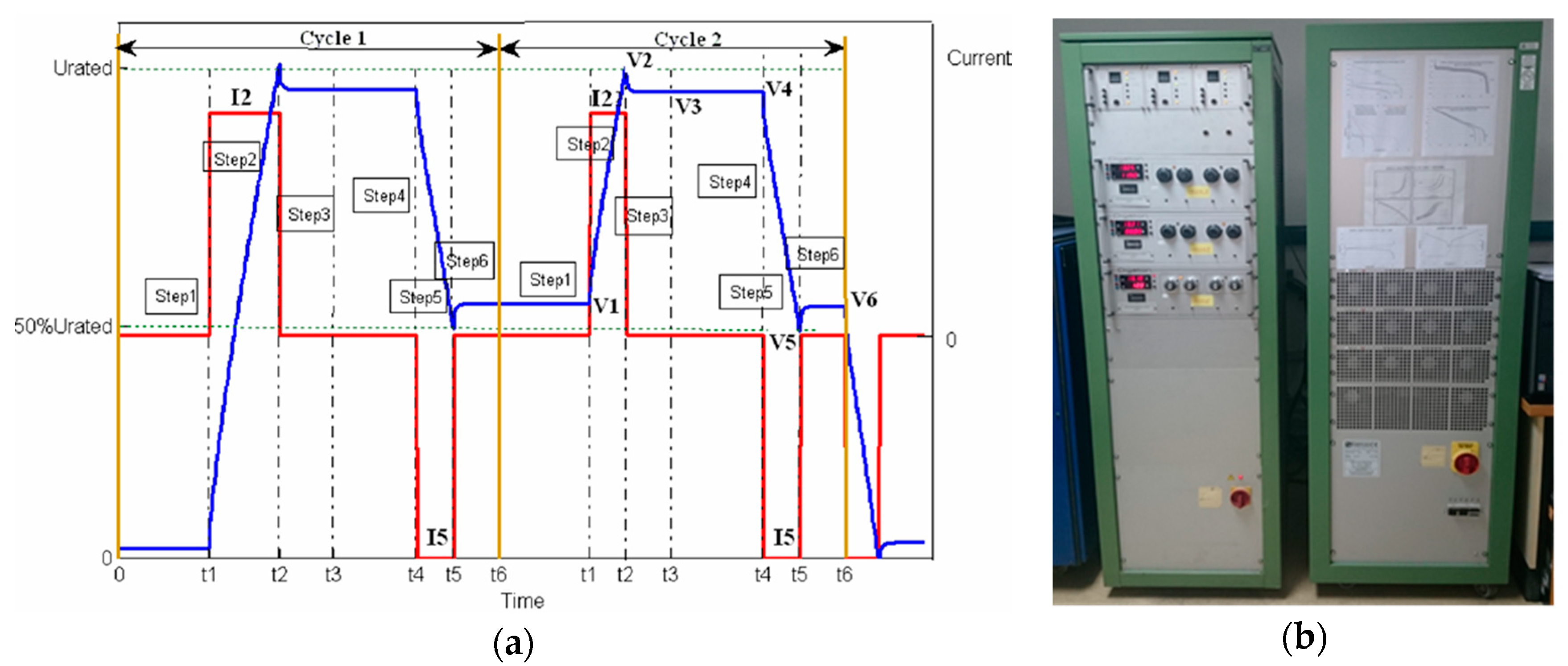
The capacitance and ESR estimation method used is the one proposed by the manufacturer and it is based on the assumption that EDLC model can be represented by a simple RC equivalent circuit. In [14] it is explained how to calculate both the C and the ESR. Figure 4a shows the voltage profile referred to time applied to SCs to calculate the C and the ESR [15]. As a continuous power source, a Digatron BTS-600 (Digatron, Aachen, Germany), displayed in Figure 4b, has been used to characterise the SCs. This power source allows one to charge/discharge the SC cells from half the nominal voltage until the nominal voltage with a current of 100 A and an error of 0.01%.

SC cells, as well as batteries, operate at low voltage (ranging from 1 to 3 V depending on the chemistry), so that in most cases a series connection of supercapacitor cells is necessary to obtain higher voltage and therefore to provide the required power. For example, a real application operating at a maximum voltage of 650 V would require 240 cells in series with 2.7 V/cell. Thus, it is necessary to take into account in the DC analysis the connection plates. In this regard, the value of this element is calculated before cycling. In this way, a correction must be made to determine the real value of ESR and be able to ignore the electrical connection and measurement contact.

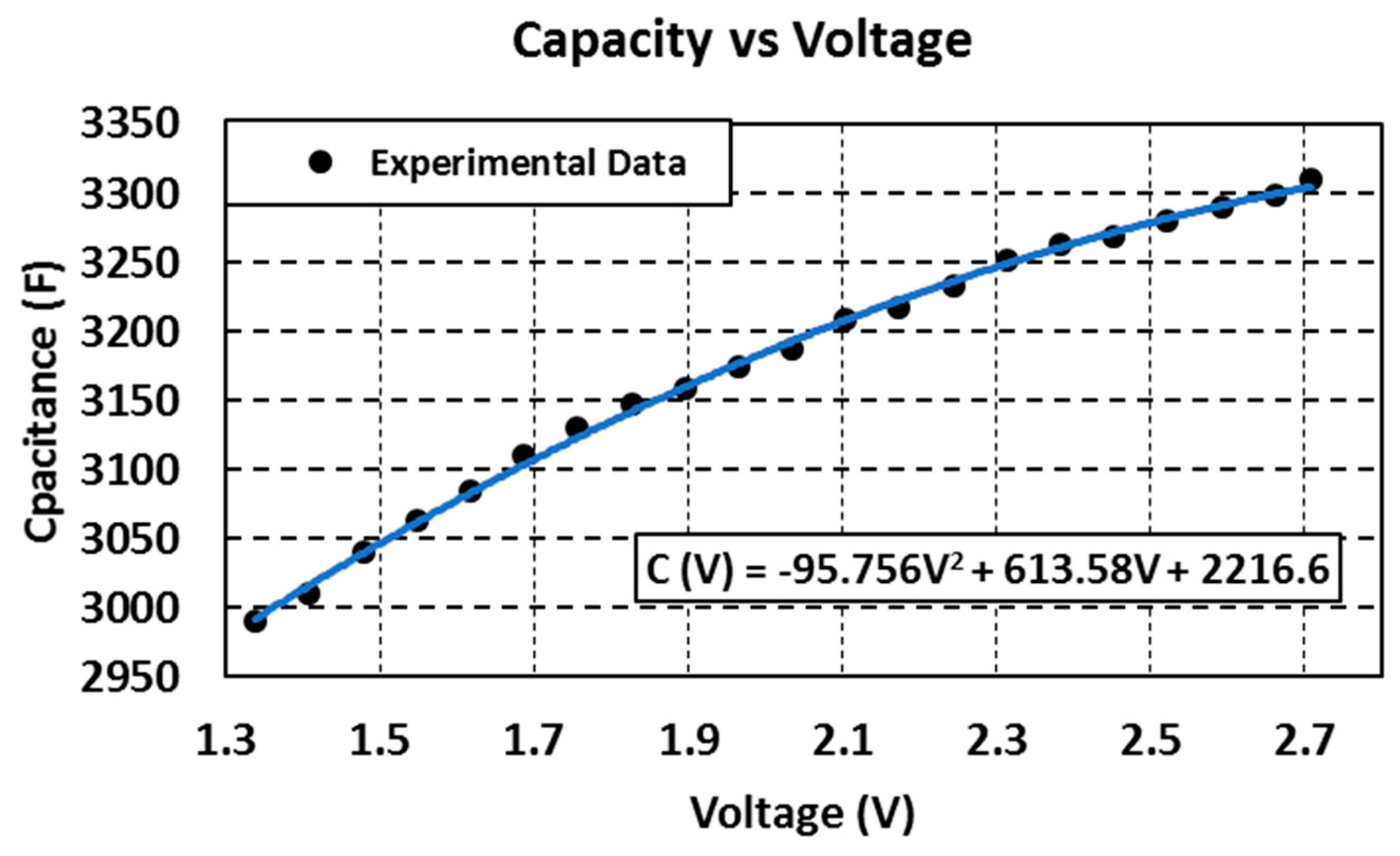
Regarding the capacitance, it should be taken into consideration that SCs are not linear capacitors, but their capacitance depends on the voltage, as shown in Figure 5 [20,25,26]. In the case of cells, manufacturers provide a value of capacity and resistance which is calculated for each cell by using the method mentioned before. Nevertheless, this capacity is just a mean value of capacity.

SCs allow the discharge from nominal voltage down to zero volts, but considering that the stored energy is proportional to the square of cell voltage, they will not be discharged below half of the nominal voltage (1.35 V). Under this condition, they can provide and store 75% of its maximum energy without generating a low voltage ratio with DC link [6].

The nominal capacitance obtained from the datasheet is an average value between the maximum and the minimum voltages of the SC. For this reason, the datasheet gives not only a nominal capacitance value, but a maximum (at the highest voltage) and a minimum (at the lowest voltage) value of this capacitance. At the beginning of the operation life this maximum value is above 3000 F. In order to model this evolution of capacitance, a charging experimental process has been carried out. The average capacitance is calculated with small increases of voltage. Figure 5 shows this evolution. It has a quadratic relationship with voltage as given by the equation below:

$$C \left(V\right)= -95.756·V^2+613.58·V+2216.6$$

(1)

Regarding the SC self-discharge effect, the self-discharge current is the current required to keep the SC at a given voltage value. The longer the SC is maintained at a given voltage, the lower the SC leakage current. This effect is influenced by the temperature, the voltage of the cell, the loading history and the ageing. The self-discharge current is given by the manufacturer in the datasheet as a constant value. This value is the charging current required to maintain the SC cell at nominal voltage, after having maintained the SC for 72 h at nominal voltage at a controlled temperature between 23 °C ± 2 °C [27]. This value (2.7 V) is characteristic of the BCAP3000F cell and the maximum value is 5.2 mA, which is calculated after 72 h of assay. As commented before, the leakage current decreases with time, which implies that a conservative estimation is to neglect the variation of the leakage current and set the value to its maximum (5.2 mA in this case).

In order to estimate the leakage current value, an assay has been performed to compare the testing value with the datasheet one. This assay follows the instructions in the technical documentation supplied by the manufacturer [28]. The assay is described in three steps [27]:

• An electric circuit is built, composed by a SC cell, a shunt precision resistance ($R_{shunt}=1\mathrm{m}\mathsf{\Omega }$) in series with the cell, a jumper in parallel with the resistance, used to charge the SC, and a voltage source. Additionally, an acquisition system is used to record the value of the leakage current over time.
• The cell is charged to its nominal voltage ($2.7\mathrm{V}$). Then, it is maintained in this state during an hour. After that hour, the jumper is removed and the current crosses through the shunt resistor and is maintained in that state for 72 h.
• After those 72 h, the assay is ended and the last value measured (72 h) is the maximum leakage current. This value is calculated using Equation (2):

$$I_{leakage}=\frac{V_{measured}}{R_{shunt}}$$

(2)

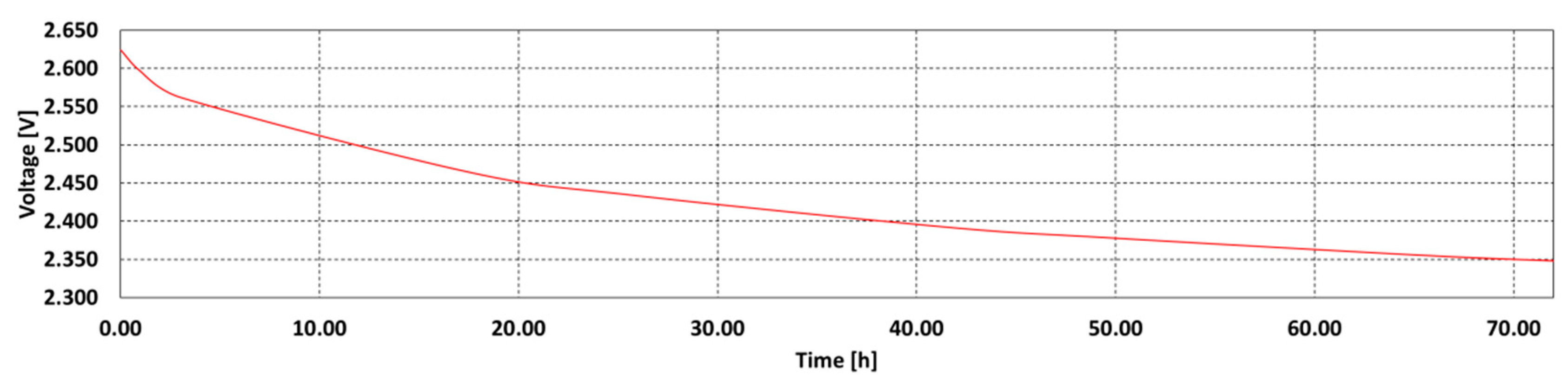
Another effect related to the leakage current that occurs during the first 72 h of the assays is the redistribution of the electrical loads. This effect is also relevant for the energy storage system during the whole operation cycle in industrial applications. Assays were carried out on several SC cells (BCAP3000F $2.7\mathrm{V}$), and, for the sake of example, experimental results for one of them are shown in Figure 6.

Using these results, an approximation of the SC voltage evolution with respect to time could be done. As mentioned before, manufacturers provide only the maximum value of the leakage current, which is given to nominal voltage in the supercapacitor. The lower the voltage in the SC, the lower this leakage current. For this reason, the leakage current could be modelled as a variable shunt resistor in function of the voltage in the SC. However, this sole element is not enough to properly represent the leakage current and the process of redistribution of the electrical loads. The electrical circuit that best models the leakage current and the redistribution of the charges is a resistance (R_L) in parallel with a resistance (R_p1) connected in series with a capacitor (C_P1) as is shown in Figure 7. The capacitance value and the resistance is variable with the voltage. This element connected in parallel to the rest of the electrical circuit model the SC behaviour at very low frequency. The value of these parameters and the rest of the electrical circuit will be discussed in Section 4.

In the next section, an electrical circuit model which best fits with the measured frequency response of the SC is proposed. The value of all the elements of the electrical circuit, R_L, R_P1 and C_P1 included, for two SCs connected in series will be commented. As will be explained later, the series connection of two SCs will be considered as the minimum functional unit.

3.2. AC Analysis

The details of the procedure to analyse the frequency performance of the SCs are explained below. The experimental data are compared with the data provided by the manufacturer to extract conclusions about the validity of the tests performed and the proposed electrical circuit model. All the experiment results have been obtained for a single cell previously charged to 2.7 V. The state of charge of the supercapacitor is very important because of the variations with the voltage in the SC. The higher the voltage, the higher the capacitance, as shown in the Figure 5. For frequencies below 100 Hz an AC bipolar power source, a BOP 20-20 M s/n E130343 (KEPCO, Flushing, NY, USA) has been used to make the frequency analysis. This power source generates a sinusoidal current signal following the reference from a signal generator. The function generator used is an 33522A s/n MY50005409 (Agilent, Santa Clara, California, USA). A high precision, 34972A s/n MY4901941 datalogger (Keysight, Santa Rosa, California, USA) is also used for the data acquisition to avoid delay between the real and the measured signal. For frequencies from 100 Hz to 100 kHz a HP 4284A Precision LCR meter (Hewlett Packard, San José, California, USA) has been used. In frequencies above 100 Hz, this system provides more precision than the aforementioned power source. According to the switching frequency used in the power electronic converter, which will drive the charge/discharge current through the capacitor, it is not necessary to obtain the response for frequencies above 20 kHz.

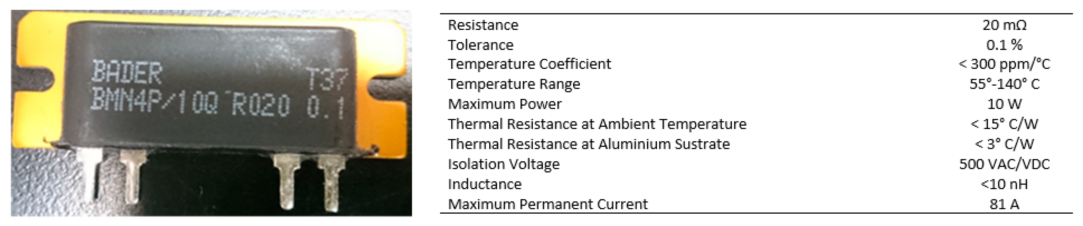
In both cases, a shunt resistance with a very low inductance (<10 nH) is used for the measurement of the current. The main electrical characteristics of this resistance are shown in Figure 8. It is a very stable resistance with a 4-wire measurement to avoid measurement errors. The SC is supplied with sinusoidal voltage of 10 mVpeak-peak from 0.001 Hz to 10 kHz with intermediate frequency values (0.001, 0.003,…., 10 kHz). As in the DC analysis, the connection plates between supercapacitors should be taken into account. A specific test has been carried out connecting two SCs in series.

The experimental results obtained for one single cell are shown in red in Figure 9. This result is compared with the experimental data provided by the manufacturer (blue line). Manufacturer data are given for a single BCAP3000 cell charged to 2.7 V at 25 °C. The resistance of the connection plates is not included, so it is necessary to add its value to the provided input data. On the other hand, it is worth mentioning that the manufactured only provides data from 0.013 Hz to 10 kHz, so below and above these frequencies there is no reference values to compare the experimental results against. Finally, the manufacturer only supplies the impedance magnitude versus frequency and the imaginary impedance versus frequency. From these two graphs, the resistance and the capacitance versus frequency evolutions need to be obtained. For frequencies below 0.1 Hz, it is very difficult to calculate the resistance from Maxwell curves without errors because the capacitance (hundreds of Farads) is much higher than the resistance (hundreds of μΩ). The experimental resistance and capacitance values are compared in Figure 9a,b respectively. The capacitance value is very similar in both cases: the value obtained experimentally and the value supplied by the manufacturer. However, in case of the resistance, the differences are greater. Especially for frequencies below 0.03 Hz and above 500 Hz. The capacitance value is maximum below 0.01 Hz and it begins to considerably decrease from 0.03 Hz. The resonance frequency is located around 80–100 Hz, where the SC begins to have inductive character.

As discussed earlier, in industrial applications it is necessary to connect cells of supercapacitors in series to reach a suitable voltage. However, the unequal voltage distribution in the cells will affect the performance and reliability of the stack. This unbalance is due to manufacturing deviations in capacitance, ESR and self-discharge from cell to cell. Self-discharge is a leakage effect dominated by redox reactions at the electrode surface through which electrons cross the double layer [29]. Capacitance variations have a greater effect on the voltage distribution during cycling, and leakage current variations during standby, as in backup applications. Since the voltage distribution between cells is unequal, there may be cells with higher voltage, very close to the upper limit voltage. Furthermore, a high voltage applied to the supercapacitor accelerates the decomposition of the electrolyte, provoking the decrease of capacitance and, as a result, a greater voltage unbalance. Subsequently, an active cell voltage balance or a maximum voltage protection system is required to achieve a good voltage distribution and to prevent any cell from reaching its absolute maximum voltage. The manufacturer supplies an active system to evenly distribute the total voltage between cells. It is not really an active balancing system but an overvoltage protection system. It consists of an electronic board which consumes power when the voltage in the cells is above 2.7 V. 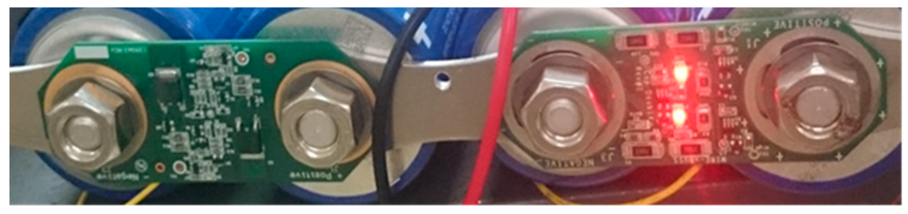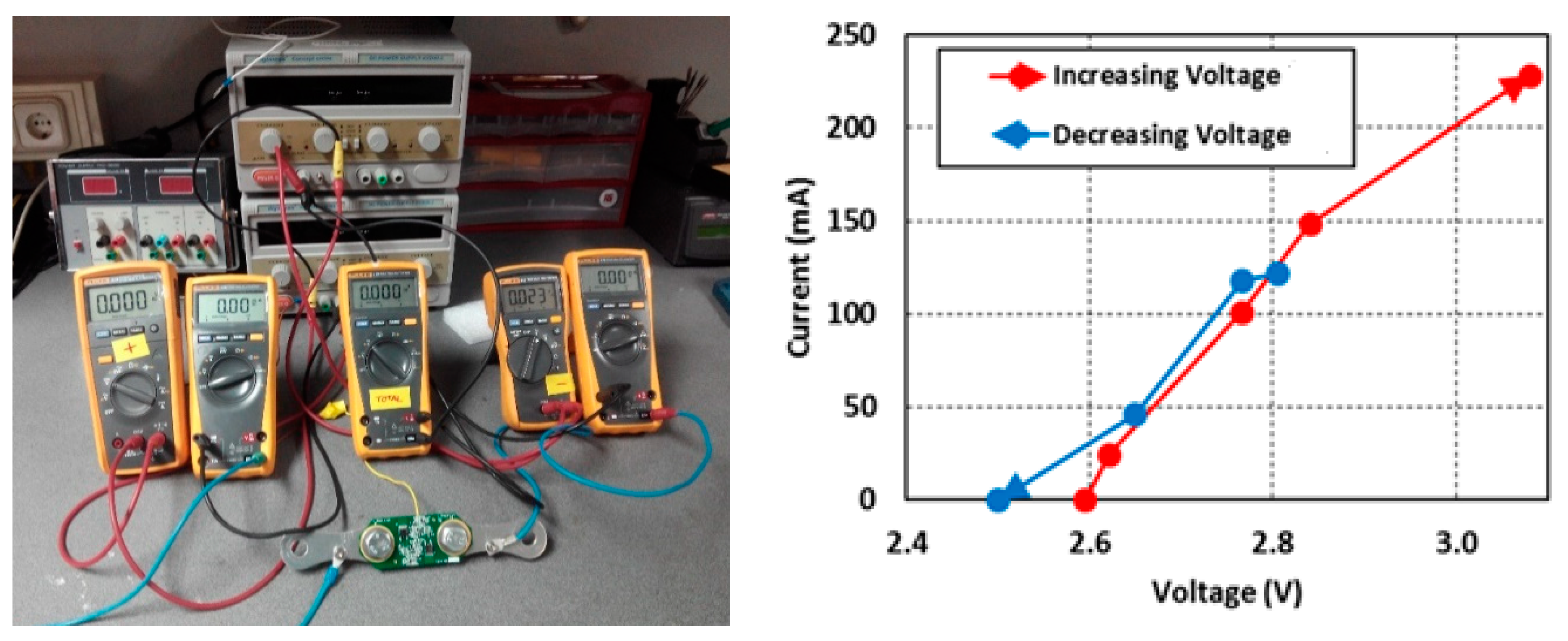Figure 10 shows the connection of SCs in series with the active balance circuit.

When the voltage in the cell is above 2.6 V a certain quantity of current drains through a resistor in a voltage balance circuit, presented in Figure 11 connected in parallel with the SC., in order to discharge the cell. The higher above 2.6 V the voltage, the higher this current. The evolution of this current with voltage is shown in Figure 11. The voltage balance circuit response was obtained with a laboratory source.

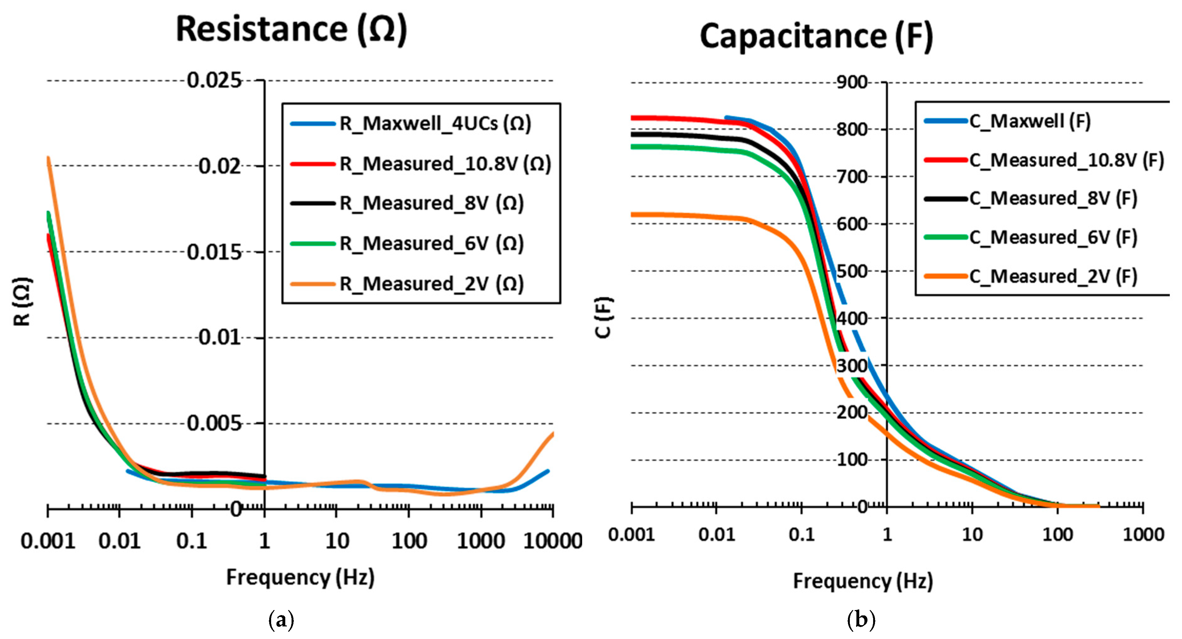
In order to evaluate the influence of the voltage on the capacitance, the resistance of the connection plates and the voltage balance circuits, four cells of SCs have been connected in series to experimentally determine the frequency response. Four different cases have been studied depending on the preload voltage (V_bias) in the SCs (2 V, 6 V, 8 V and nominal voltage 10.8 V). 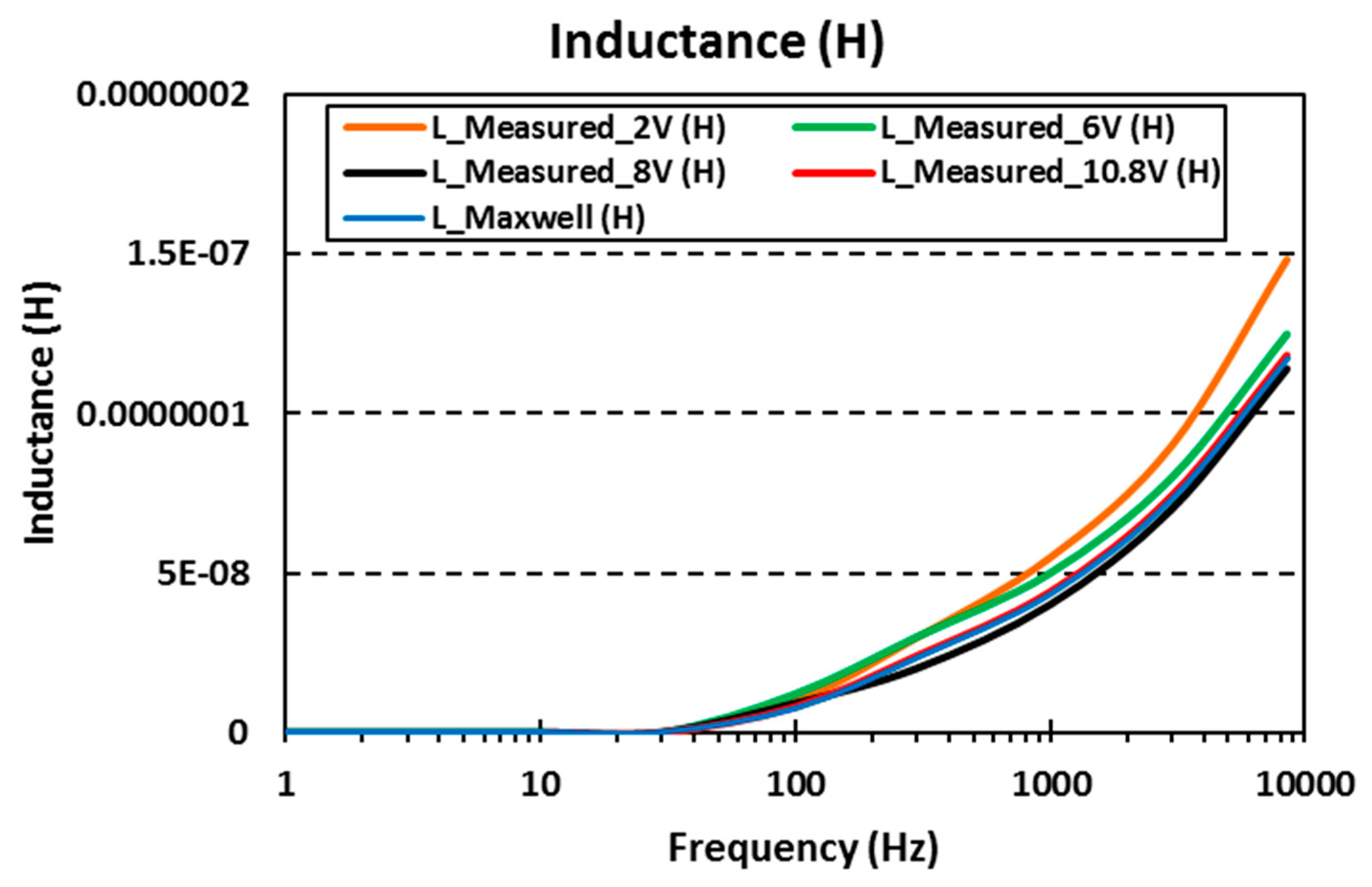The total measured resistance and capacitance (R_TOT = 4·R_SINGLE and C_TOT = C_SINGLE/4) for each case compared with the data supplied by the manufacturer are shown in the Figure 12a,b. The total inductance as a function of the frequency is shown in the Figure 13. As only data of one cell is available from the manufacturer, it is necessary to extrapolate the resistance, the capacitance and the inductance values for four cells connected in series, including the resistance of the connection plates.

In this case, the measured resistance is approximately four times greater than the measured value in one single cell. On the other hand, observing the graph one can argue the voltage may have some influence in the resistance in the frequency range below 0.01 Hz. The SCs precharged to 2 and 2.7 V have a very similar resistance value. The resistance of the SCs precharged to 1.5 V is higher than the previous value and the highest resistance value is given in the SCs precharged to 0.5 V. Although it is true that the minimum voltage in operation of the SCs will be 1.35 V, so as not to penalise the efficiency of the power converter which drives the current through the SCs. At half voltage in the SC, only a quarter of the total energy is available. Comparing the capacitance of one single cell with the total capacitance of four SCs connected in series, the former is in the order of four times greater than the latter. Conversely, the total inductance of one single cell is in the order of four times larger than the total inductance value in the series connection of four SCs.

Regarding the value of the capacitance, the higher the voltage in the cells, the higher the capacitance. As already mentioned above, in the voltage range from 1.35 V to 2.7 V the relation between capacitance and voltage is quadratic. Below 1.35 V, the capacitance decreases in a more pronounced way with voltage. As in the case studied of one single cell, the resonance frequency is around 80 Hz.

Figure 13 shows the inductance evolution (sum of the inductances of the four cells) with the frequency. The inductance value varies depending on the voltage in the cells. The higher the voltage, the lower the inductance, although the differences are smaller compared to existing difference in the capacitance. From 80 Hz on, the SC behaves like an inductive element.

4. Frequency Model Design of the Supercapacitor to Adjust the Model Response with the Experimental Response

As explained in the previous section, with electrochemical systems such as SCs, conventional electrical elements (resistances, capacitors and inductances) cannot represent the frequency response of the electrochemical phenomena that occur in this energy storage system. Some of these phenomena are charge and mass transfer and processes of surface diffusion and adsorption. Therefore, equivalent electrical circuits are necessary to model these processes by using in dielectric impedance spectroscopy. These elements are Warburg impedances, constant phase elements (CPE), YAC and ZARC [30,31,32,33].

In most of the industrial applications it is necessary the series connection of SCs to reach the suitable voltage levels. For that purpose, a functional unit with two SCs connected in series and an active voltage balance board is proposed as the basic unit to model the series connection of n SCs. The complete set of chains of n SCs will be the sum of n/2 functional units [34]. The suggested model has to fit the experimental data, taking into account the dependence of the capacitance on the voltage. In order to find an equivalent electric circuit to model the behaviour of the series connection of the SCs, the software EC-Lab^® (Biologic Science Instruments, Seyssinet-Pariset, France) is used [35]. This software enables the user to compare the frequency response of the SCs obtained experimentally and the selected circuit so that the response of both is the same. Figure 14 shows the equivalent electrical circuit of two SCs connected in series with an active voltage balancing board. This electrical circuit model is very similar to Rafik’s model, but it has fewer parameters, eleven as opposed to fourteen. Most electrical circuit parameters in this model have a voltage dependence to get the same frequency response than the frequency response of the SCs obtained from the experimental data. This is because the frequency response of the supercapacitor is variable with the voltage. On the other hand, the electrical circuit proposed models the frequency response of the SCs at high frequencies, above 1 kHz. Most existing SC electrical circuits in the literature, including Rafik’s model, do not model the frequency response properly at these frequencies. Taking into account that a power converter will drive the current through the SCs there will be a high frequency component of this current will pass through the SCs with no undesirable effects. This high frequency component will increase the power losses of SCs and the temperature on it provoking an accelerated ageing. On the other hand, the revised models in Section 2 do not describe the methodology to calculate the parameters of the electrical circuit model.

As mentioned in Section 3 (DC analysis), R_L, R_p1, C_p1 model the behaviour of the two SCs at very low frequencies, below 1 mHz. The value of these parameters is calculated for very long periods of charge and discharge (very low frequency response). R₁ in series with C₁ represent the behaviour of the SC in the frequency range of 1 mHz to 1 Hz, frequency range where the ESR value provided by the manufacturer is calculated [27]. C₁ is the capacitor with the highest capacitance in the circuit and it is important to set the initial voltage value of this equivalent capacitor in function of the voltage in the two SCs. All parameters in the electrical circuit model are influenced by voltage, but this particular parameter is the one that shows a greater dependence on it. The diffusion phenomena which occurs from 1 Hz to 300 Hz will be modelled with a resistance in parallel with a capacitance (R_C2//C₂) and a resistance in parallel with an inductance (R_L2//L₂). In this frequency range, the AC ESR value is found. The first of these circuits (R_C2//C₂) represents the capacitance zone and the second one represents the inductive zone that is given from the resonance frequency (80–100 Hz). Finally, the resistance R_L1 connected in series with the inductive L₁ model the behaviour of the SCs at high frequencies.

The value of R_L and C_p1 is variable with voltage to fit the voltage decay in the SCs with the measured voltage between the positive and negative terminals. As mentioned in Section 3, the total operating voltage of the two SCs is set at between half the nominal voltage and the nominal voltage (2.7 V to 5.4 V). The maximum value of R_L is given at the nominal voltage and the minimum voltage at half the nominal voltage. The value of the capacitor C_p1 is variable with the total voltage in the SCs (Vbias). R_p1 is an invariable resistance with voltage of constant value.

Table 2. Value of the electrical parameters which model the frecuency response of the two SCs at very low frecuencies. V is the measured voltage between the positive and negative terminal.

RL (Ω)	RP1 (mΩ)	CP1 (F)
203.7·V	823.18	93.2028·V

resumes the value of these parameters with voltage. Now, it is necessary to calculate the rest of the electrical circuit elements in function of the frequency response of the SCs.

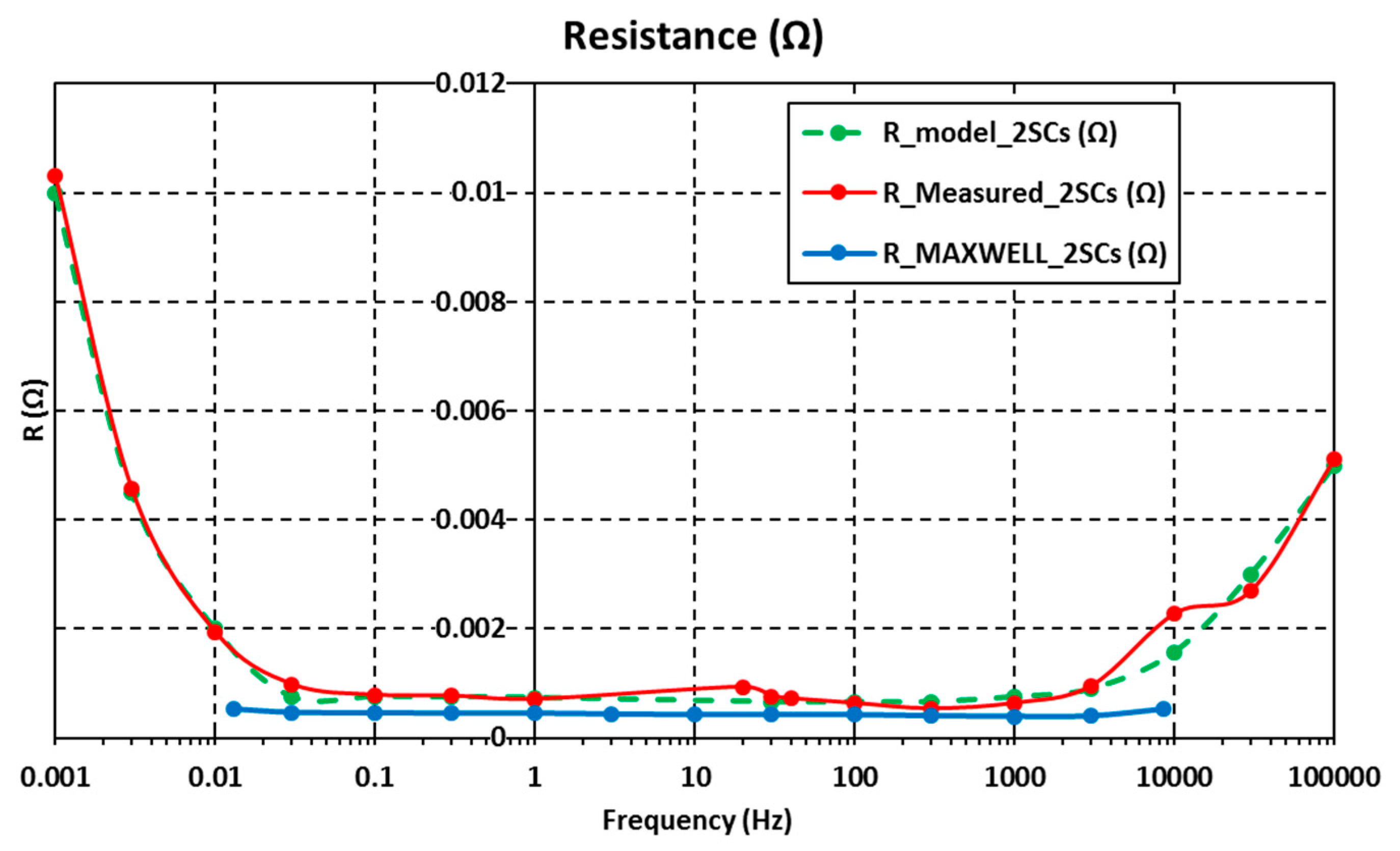
In terms of higher frequency analysis, Figure 15 shows the comparison between the equivalent resistance of the proposed model and the experimental resistance obtained with two SCs connected in series and with an initial voltage of 2.7 V. In the same way, Figure 16 shows the comparision between the evolution of the equivalent capacitance of the electrical circuit model with frecuency and the evolution with frecuency of the real capacitance (from experimental tests).

Since the variation of the voltage in the SCs affects the frequency response, it is necessary to calculate the correlation of each circuit element with voltage. In order to derive this mathematical relationship, the value of each element in the circuit is calculated with the software EC-Lab^®. Four cases have been studied based on the four experimental tests carried out (2.7 V, 2 V, 1.5 V and 0.5 V in each cell). The circuit parameters obtained for each voltage V_bias (sum of the voltage in each SC) are shown in

Table 3. Values of the electrical circuit elements for the different initial voltages in the cells.

Vbias (V)	R1 (Ω)	C1 (F)	Rc2 (Ω)	C2 (F)	RL2 (Ω)	L2 (H)	L1 (H)	RL1 (Ω)
1	5.45 × 10−4	708.5	4.94 × 10−5	1850	4.05 × 10−4	7.06 × 10−8	9.29 × 10−8	6.16 × 10−2
3	5.74 × 10−4	1582	6.54 × 10−5	1152	2.40 × 10−4	6.04 × 10−8	8.99 × 10−8	5.96 × 10−2
4	5.68 × 10−4	1644	7.68 × 10−5	981	2.53 × 10−4	5.95 × 10−8	8.25 × 10−8	5.47 × 10−2
5.4	5.96 × 10−4	1801	8.97 × 10−5	870	2.63 × 10−4	5.83 ×10−8	8.02 × 10−8	5.32 × 10−2

.

Subsequently, the software Statgraphics Centurion^® is used to determine, by statistical analysis, the relation of all these elements with the voltage (V_bias) of the SC. Statgraphics Centurion^® is a statistics software that performs and explains the basic and advanced statistical functions [36]. Other softwares can be used to calculate the variation of the electrical parameters with V_bias (SPSS^®, S-PLUS^®, MINITAB^®, MATLAB^® or simply EXCEL^®). Statgraphics Centurion^® software is used against other options, but the results obtained with any of the mentioned softwares are very similar. From the analysis carried out, it has been proved that all electrical circuit parameters, to a greater or lesser degree, have a quadratic relationship with voltage. However, the capacitance of the SCs (capacitors of the electrical circuit) has a greater dependence on the voltage than resistance and inductance have. The model equation to calculate any parameter of the electrical circuit in function of the voltage is A x² + B x + C. The values of these coefficients for each element of the electrical circuit are shown in

Table 4. Parameter values of the coefficients A, B y C for the elements of the electrical circuit.

	R1 (Ω)	C1 (F)	Rc2 (Ω)	C2 (F)	RL2 (Ω)	L2 (H)	L1 (H)	RL1 (Ω)
A	1.12 × 10−5	−22.96	3.68 × 10−7	141.02	2.54 × 10−5	3.10 × 10−9	−8.98 × 10−11	1.12 × 10−5
B	−7.93 × 10−5	−269.82	1.12 × 10−5	−1282.12	2.32 × 10−4	−3.04 × 10−8	−6.08 × 10−10	1.12 × 10−5
C	4.82 × 10−5	965.2	3.06 × 10−5	3722.26	5.98 × 10−4	1.09 × 10−7	3.93 × 10−8	1.12 × 10−5

.

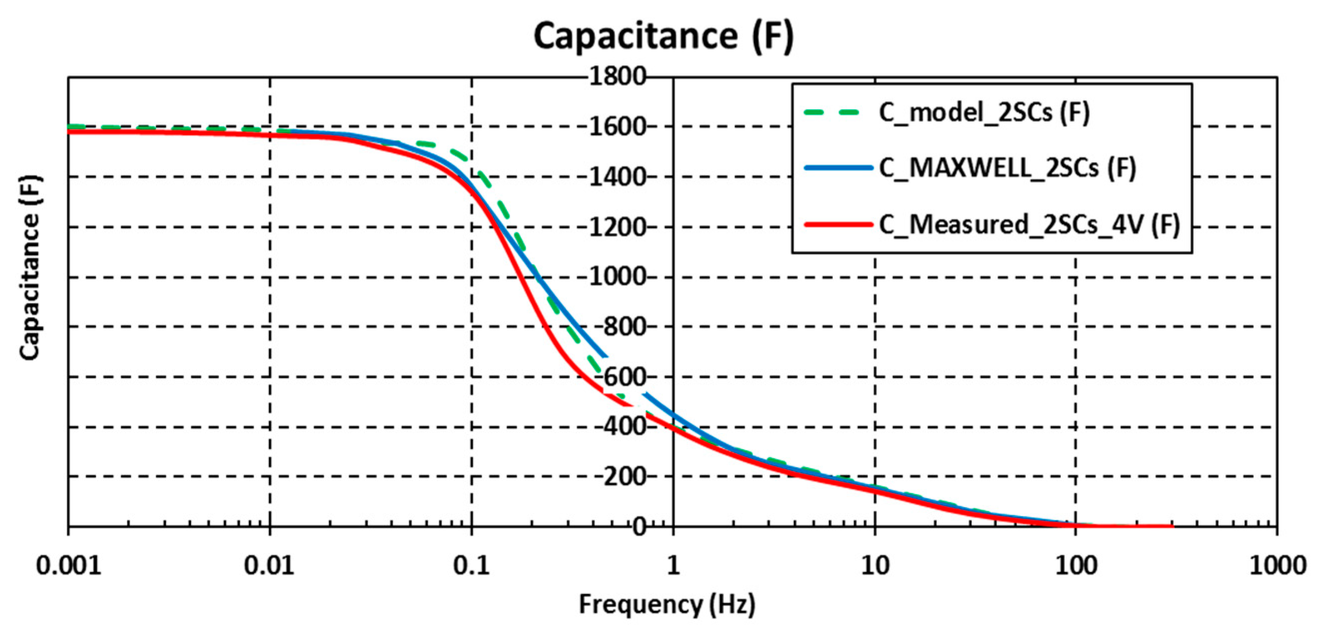
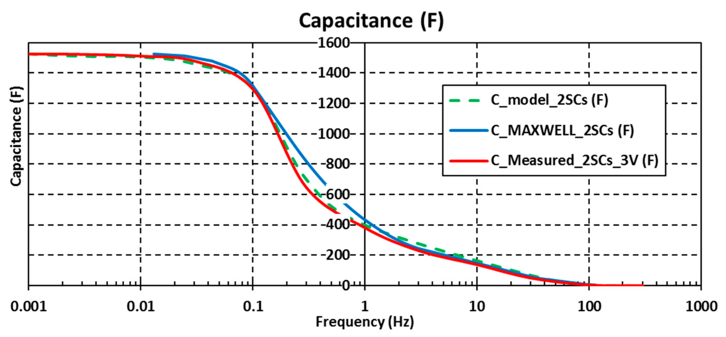
Figure 17 and Figure 18 show the comparison in the frequency response of the measured capacitance through EIS technique and the electrical model. In both figures, the initial voltage in the cells is different in order to verify that the model fits the real response and it is valid in the entire operating voltage range of SCs.

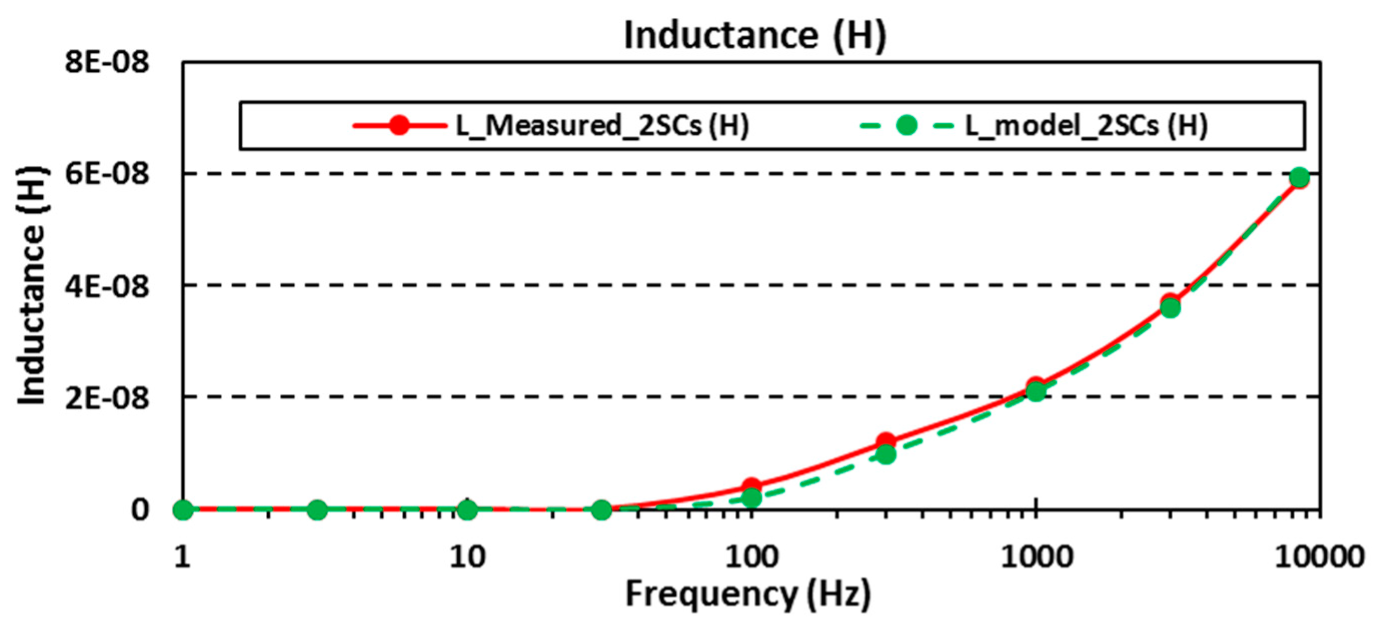
In the same way as in the case of the capacitance, it is necessary to check if the model fits the real response at high frequencies, where the SC has an inductive behaviour. Figure 19 shows the difference between the SC and the proposed model.

5. Conclusions

Through the study conducted in this paper, a methodology to determine an electrical circuit which models the frequency response of supercapacitors (SCs) has been described. A basic energy storage system unit, comprising the series connection of two SCs, is proposed. It includes the connection plates and a voltage balancing circuit. The experimental results obtained through EIS methodology have been compared with the proposed model in order to validate it over the entire operation frequency range. This frequency range includes frequencies above 1 kHz, where high-frequency components are found due to the switching frequency of the power electronics. The analysis has evaluated the voltage influence in the impedance of the SCs (ESR, capacitance and inductance). The electrical model can be extrapolated to the series connection of more than two SCs, something very common in the industrial applications. Finally, another conclusion in view of the results obtained is that the faster the charge/discharge of this energy storage system (SC) the lower the capacity value and therefore the lower the energy storage capability.