Single-Diode Models of PV Modules: A Comparison of Conventional Approaches and Proposal of a Novel Model

Abstract

In this paper, the seven traditional models of photovoltaic (PV) modules are reviewed comprehensively to find out the appropriate model for reliability. All the models are validated using the Matlab code and graphical comparisons between models are made. The accuracy and convergence of each model is evaluated using the data of manufactured PV panels. Then, a novel model is proposed showing its consistent performance. The three most key parameters of the single-diode model are self-revised to adapt to various types of PV modules. This new method is verified in three types of PV panels’ data measured by the National Renewable Energy Laboratory (NREL), USA. The validated data show promising results when the error RMSEs’ range of the proposed model is under 0.36.

1. Introduction

The rapid exhaustion of conventional energy resources, such as coal, crude oil, and natural gas, has been threatening to energy security in the world. Since renewable resources are clean and inexhaustible, the penetration of renewable energy has been arising from time to time in academia, industry, business, and government. Concerning a 100% renewable goal in the next few decades worldwide, renewable energy has been becoming a hot topic in the research community. In this context, Photovoltaic (PV) energy becomes one of the prominent renewable energy resources. With an increase of more than 30% in 2018, the power generation from PV is estimated to be over 580 TWh [1]. Because of the technical improvements in PV and the dramatic drop in the price of solar PV panels, solar PV systems continue developing. In terms of generation, by 2050, solar PV could become the second-largest power generation source, behind the wind power. This growth would meet 25% of the total energy demand globally [2]. To estimate the economic feasibility of a solar PV system, the evaluation of the output power of a PV plant needs to be addressed. Identifying the standard I-V characteristics of specific PV panels is a key to estimating accurately the output power of PV panels. As a result, researchers have proposed various methods to predict the performance of a PV module based on modeling it, all of which can be divided into analytical methods and metaheuristic algorithms [3]. Some optimization techniques are employed in metaheuristic algorithms, and have been applied to obtain the model parameters as follows: Simulated annealing [4], bacterial foraging algorithm [5], genetic algorithm [6], differential evolution [7], partial algorithm [8], artificial bee colony [9], simplified swarm optimization [10], etc. While these models impose no restrictions on the problem formulation [11], metaheuristic algorithms might take long computational time and have convergence difficulty. Meanwhile, in [11,12,13,14,15,16,17,18,19,20,21,22,23,24,25,26,27,28,29,30,31,32,33], analytics methods utilize a set of mathematical equations and assumptions from the datasheet provided by manufacturers. The trade-off between model accuracy and computational time makes the analytics methods much more popular in engineering applications than metaheuristic methods.

The best way to analyze the behavior of the PV generator is to adopt an equivalent circuit and to analyze relevant equations describing it [14]. A PV cell is described by an equivalent circuit consisting of a current source, at least one diode, and one resistor [15] based on the intrinsic characteristics. The single-diode model (SDM) [13,16,17] and the double-diode model [11,18,19] have gained the most researchers’ attentions, specifically the SDM. While the double-diode model has a certain advantage, that is representing the recombination loss in the depletion region [20], the double-diode model requires solving implicit nonlinear seven-parameters [11]. This has led to more difficulties in the calculation of the initial values, long computational time, and algorithm complexity. Meanwhile, the SDM gets the desired compromise between accuracy and simplicity [20].

Different methods have been proposed to extract the five parameters of the SDM. In [12,13,14,15,16,17,18,19,20,21], a set of implicit equations accompanied by assumptions and simplifications were used to formulate the equations obtaining the model parameters.

An iterative and an analytical method are conducted by [13,17,22], who proposed a method to estimate parameters through a trial-and-error approach.

Meanwhile, model parameters were identified by using mathematical manipulations in [14,15,23,24,25,26]. Specifically, the Lambert-W function at five experimental points was applied in [14,15,24,25,26].

References [3,34,35] reviewed the remarkable models from 2002 to 2017. The comparisons among models were discussed to choose the model that fits the applications in reality. However, all models are only investigated in their performances on one type of PV module. Consequently, the selection of a suitable model for an application is decided only based on computational time and model accuracy, which is insufficient to assess properties of various types of PV panels. In this article, we conduct experiments on three main types of PV modules under varied solar irradiance and cell temperature, such a performance of a PV system largely depends on cell temperature (T)–solar irradiance (G) conditions (T-G) [17]. Since the new method has proved its advantages, it is verified in three types of PV panels, the data of which are tested by the National Renewable Energy Laboratory (NREL), USA. Since the results have shown the promise of this method, it could be used in predicting the performance of a PV panel.

The main contributions of this paper are four folded:

• Review previous models to build I-V curves of PV modules
• Compare the accuracy of these models
• Propose a higher performance model
• Validate the proposed model by the real PV module’s data

The rest of this paper is organized as follows. Section 2 briefly introduces the fundamental model of the SDM. Section 3 describes reviewed models. Section 4 discusses the reviewed model and then Section 5 describes the proposed model. Section 6 shows the numerical results validating the reviewed and proposed models. Finally, the conclusion is drawn in Section 7.

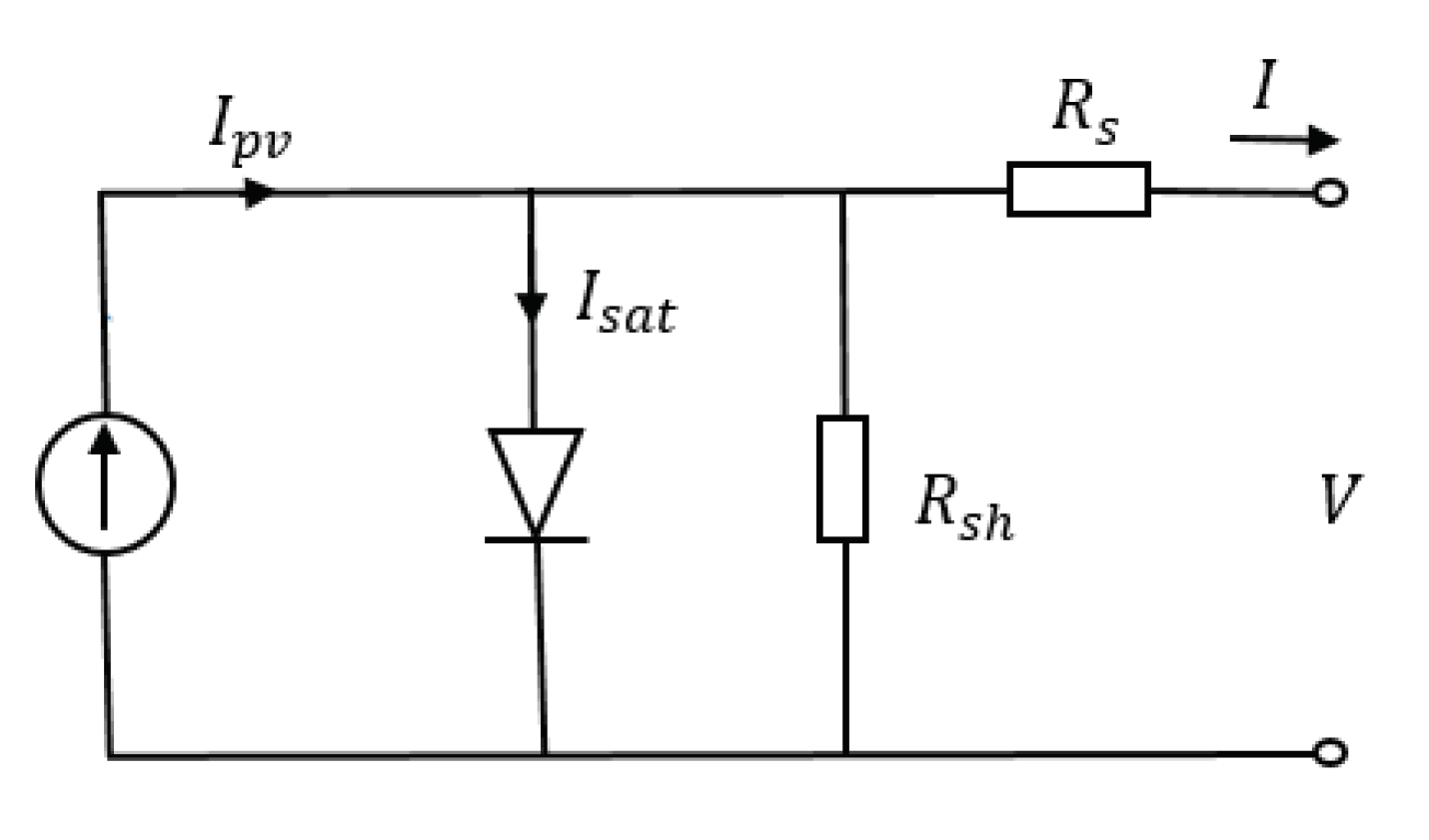
2. Equivalent Circuit of the Single-Diode Model

Figure 1 illustrates the well-known equivalent circuit of the SDM, which consists of one current source, one diode, one series resistor, and one shunt resistor. The series resistor is added to take into account the voltage which drops across the transport resistances of the solar cell. The shunt resistor represents the effect of the leakage current in the p-n interface of the diode and the edges, as well as the shunt resistance occurring across the solar cell surface [27]. Normally, the estimated value of shunt resistance is very high compared to the series resistance.

The relationship between the output current-voltage is expressed by the following equation:

$$I=I_{pv}-I_d-\frac{V+I{R}_s}{R_{sh}}$$

(1)

$I_{pv}$ is the PV current, generated by electron-hole pairs within a solar cell. $I_d$ is the Shockley diode current, which is described by Equation (2), where $I_{sat}$ is the reverse saturation current measuring the leakage or recombination of minority carriers across the $p-n$ junction in reverse bias [25], which is calculated by means of Equation (3). The SDM assumes that the Shockley current can be described by a single exponential dependence modified by the diode ideality factor a [25]. $E_{gap}$ is the bandgap energy of the semiconductor material ($E_{gap}$ = 1.12 eV for the crystalline Si at 25 ${}^{°}$C [30,31]).

$$I_d=I_{sat}\left(e^{\frac{qV}{akT}}-1\right)$$

(2)

$$I_{sat}=C{T}^3{e}^{\left(-\frac{E_{gap}}{kT}\right)}$$

(3)

In fact, PV generators are made of a number of PV cells connected in series and parallel, not referred to as a single PV cell. The operating voltage of the PV cell is a few hundreds of millivolts, while the current generating at high irradiance levels is of some amperes. As a result, to reach the desired voltage, a number of connected-series cells are arranged into PV modules. So some researchers have used a modified expression of Equation (1) as follows:

$$I=I_{pv}-I_{sat}\left(e^{\frac{V}{a{N}_s{V}_t}}-1\right)-\frac{V+I{R}_s}{R_{sh}}$$

(4)

$V_t$ is defined as the thermal voltage of the cell:

$$V_t=\frac{kT}{q}$$

(5)

3. Methodology Extracting Model Parameters from Datasheet Values

All reviewed models use information from the datasheets provided by the manufacturers. Usually, manufacturers provide the values of significant points, i.e., its short-circuit current ($I_{sc}$), its open-circuit voltage ($V_{oc}$ ), its current and voltage at the MPP ($I_{mpp}$, $V_{mpp}$), the temperature coefficient of the short-circuit current ($K_i$), and the temperature coefficient of the open-circuit voltage ($K_v$). Unfortunately, those values are provided only at the standard test condition (STC). This condition is defined as in the temperature of 25 ${}^{°}$C, the irradiance of 1000 $\mathrm{W}/{\mathrm{m}}^2$, and the air mass of 1.5.

In order to estimate effectively the performance of the PV module, the resolution is divided into two steps: Estimating five parameters of the SDM model (the ideality factor of diode a, the PV current $I_{pv}$, the reverse saturation current $I_{sat}$, the series resistance $R_s$, the shunt resistance $R_{sh}$) at the STC, then scaling this model at other T-G conditions of cell temperature and solar irradiance. In these reviewed articles, all methods provide three equations by applying Equation (4) in the open-circuit, short-circuit, and MPP, giving the results:

• At short-circuit point ( $I=I_{sc}$, $V=0$):

  $$I_{sc}=I_{pv}-I_{sat}\left[exp\left(\frac{R_s{I}_{sc}}{a{N}_s{V}_t}\right)-1\right]-\frac{I_{sc}{R}_s}{R_{sh}}$$

  (6)
• At open-circuit point ( $I=0$, $V=V_{oc}$ ):

  $$0=I_{pv}-I_{sat}\left[exp\left(\frac{V_{oc}}{a{N}_s{V}_t}\right)-1\right]-\frac{V_{oc}}{R_{sh}}$$

  (7)
• At the MPP ($I=I_{mpp}$, $V=V_{mpp}$ ):

  $$I_{mpp}=I_{pv}-I_{sat}\left[exp\left(\frac{V_{mpp}+R_s{I}_{mpp}}{a{N}_s{V}_t}\right)-1\right]-\frac{V_{mpp}+R_s{I}_{mpp}}{R_{sh}}$$

  (8)

Three Equations (6)–(8) are utilized in all reviewed methods. To obtain five model parameters, two additional equations or conditions are required. Since solving five transcendental equations contains the exponential functions and five variables, it cannot be solved straight away. Different approaches identifying parameters are presented in seven methods as follows.

3.1. Celik and Acikgoz Method-2007

Celik and Acikgoz [16] introduced an analytical method to extract five parameters of the SDM. The authors use two following definitions to estimate the values of the series and shunt resistances:

$$R_{so}=-{\left(\frac{dV}{dI}\right)}_{I=0;V=V_{oc}}$$

(9)

$$-\frac{1}{R_{sho}}={\left(\frac{dI}{dV}\right)}_{I=I_{sc},V=0}=-\frac{\frac{I_{sat}}{a{N}_{s}T}exp\left(\frac{V_{oc}}{a{N}_{s}T}\right)+\frac{1}{R_{sh}}}{1+R_s\left(\frac{I_{sat}}{a{N}_{s}T}exp\left(\frac{V_{oc}}{a{N}_{s}T}\right)+\frac{1}{R_{sh}}\right)}-\frac{1}{R_{sho}}={\left(\frac{dI}{dV}\right)}_{I=I_{sc};V=0}$$

(10)

where $R_{so}$ and $R_{sho}$ are the reciprocals of the slopes at the open-circuit point and short-circuit point, respectively. Evaluation of the series and shunt resistances is not provided by manufacturers. Since manufacturers do not provide the information to evaluate the series and shunt resistances, these data have to be graphically extracted from the I-V curve in the datasheet, which may lead to measurement error affecting the results. After that, the following five equations, Equations (11)–(15), are proposed to calculate model parameters but do not refer to any explanations about these equations.

$$R_{sh}=R_{sho}$$

(11)

$$a=\frac{V_{mpp}+I_{mpp}{R}_{so}-V_{oc}}{V_t{N}_s\left[ln\left(I_{sc}-\frac{V_{mpp}}{R_{sh}}-I_{mpp}\right)-ln\left(I_{sc}-\frac{V_{oc}}{R_{sh}}\right)+\left(\frac{I_{mpp}}{I_{sc}-\frac{V_{oc}}{R_{sh}}}\right)\right]}$$

(12)

$$I_{sat}=\left(I_{sc}-\frac{V_{oc}}{R_{sh}}\right)e^{-\frac{V_{oc}}{a{N}_s{V}_t}}$$

(13)

$$R_s=R_{so}-\left(\frac{a{N}_s{V}_t}{I_{sat}}{e}^{-\frac{V_{oc}}{a{N}_s{V}_t}}\right)$$

(14)

$$I_{pv}=I_{sc}\left(1+\frac{R_s}{R_{sh}}\right)+I_{sat}\left(e^{\frac{I_{sc}{R}_s}{a{N}_s{V}_t}}-1\right)$$

(15)

To scale the model at other temperature-irradiance (T-G) conditions, the values of $I_{sc}$ and $V_{oc}$ are calculated as follows:

$$I_{sc}\left(G,T\right)=I_{sc}\frac{G}{G_{ref}}+K_i\left(T-T_{ref}\right)$$

(16)

$$V_{oc}\left(G,T\right)=V_{oc}+a{N}_s{V}_{t}ln\left(\frac{G}{G_{ref}}\right)+K_v\left(T-T_{ref}\right)$$

(17)

As a result of Equations (12)–(15), four other parameters, except for $R_{sh}$, can be calculated at the new T-G condition.

3.2. Villalva et al., 2009

An iterative method was used by Villalva et al. to extract five parameters. The process is started with the initial values of series and shunt resistances as follows:

$$R_s=0$$

(18)

$$R_{sh}=R_{sh,min}=\frac{V_{mpp}}{I_{sc}-I_{mpp}}-\frac{V_{oc}-V_{mpp}}{I_{mpp}}$$

(19)

This process is stopped when it reaches the pre-defined tolerance of maximum power ($to{l}_p$). Substituting the values of the current, voltage, and power at the MPP ($I_{mpp}$, $V_{mpp}$, $P_{max,e}$) on Equation (8), the shunt resistance can be rewritten by the relationship with series resistance as Equation (20). This equation is used to update the value of the shunt resistance based on the value of the series resistance for each loop.

$$R_{sh}=\frac{V_{mpp}\left(V_{mpp}+I_{mpp}{R}_s\right)}{V_{mpp}{I}_{pv}-V_{mpp}{I}_{sat}{e}^{\frac{V_{mpp}+I_{mpp}{R}_s}{N_{s}a{V}_t}}+V_{mpp}{I}_{sat}-P_{max,e}}$$

(20)

In Equation (6), the second term is assumed to be able to be neglected since it is too low compared to the PV current [30,31]. Therefore, the PV current and the reverse saturation current are, respectively, calculated as the following equations.

$$I_{pv}=\frac{R_s+R_{sh}}{R_{sh}}{I}_{sc}$$

(21)

$$I_{sat}=\frac{I_{pv}-\frac{V_{oc}}{R_{sh}}}{e^{\frac{V_{oc}}{a{N}_s{V}_t}}-1}$$

(22)

In the paper published in 2009 [22], the author chose the initial value of the ideality diode factor equal to 1.3. However, in the updated version in 2014 on the website of the author, a is calculated by the following equation:

$$a=\frac{K_v-\frac{V_{oc}}{T}}{N_s{V}_t\left(\frac{K_i}{I_{pv}}-\frac{3}{T}-\frac{E_{gap}}{k.T^2}\right)}$$

(23)

3.3. Femia 1 et al.-2012

The value of the shunt resistance is considered high. By assuming $R_{sh}\to$ infinity, the last term in Equation (4) can be neglected. Equation (4) now becomes:

$$I=I_{pv}-I_{sat}\left[e^{\frac{\left(V+I.R_s\right)}{N_{s}a{V}_t}}-1\right]$$

(24)

At the short-circuit condition, Equation (24) becomes:

$$I_{sc}=I_{pv}-I_{sat}\left(e^{\frac{I_{sc}{R}_s}{a{N}_s{V}_t}}-1\right)$$

(25)

Since $I_{pv,ref}\gg I_{sat,ref}\left(e^{\frac{I_{sc}{R}_s}{a{N}_s{V}_t}}-1\right)$, the PV current could be assumed equal to the short-circuit current in the STC:

$$I_{pv,ref}=I_{sc,ref}$$

(26)

The diode ideality factor is calculated by means of the following equation, which is explained in detail in [14].

$$a=\frac{\left(K_v-\frac{V_{oc}}{T}\right)}{N_s{V}_t\left(\frac{K_i}{I_{pv}}-\frac{3}{T}-\frac{E_{gap}}{k{T}^2}\right)}$$

(27)

The reverse saturation current is calculated by rewriting of Equation (24) under open-circuit condition with the assumption that $e^{\frac{I_{sc}{R}_s}{a{N}_s{V}_t}}\gg 1$.

$$I_{sat}=I_{pv}{e}^{-\frac{V_{oc}}{a{N}_s{V}_t}}$$

(28)

so that the temperature coefficient C in Equation (3) can be evaluated as follows:

$$C=\frac{I_{sat}}{T^3{e}^{-\frac{E_{gap}}{kT}}}$$

(29)

The series resistance can be determined by using the MPP data:

$$I_{mpp}=I_{pv}-I_{sat}\left[e^{\frac{V_{mpp}+I_{mpp}{R}_s}{a{N}_s{V}_t}}-1\right]\approx I_{pv}-I_{sat}{e}^{\frac{V_{mpp}+I_{mpp}{R}_s}{a{N}_s{V}_t}}$$

(30)

Substituting Equation (28) into Equation (30) yields:

$$I_{mpp}=I_{pv}-I_{pv}\left[e^{\frac{\left(-V_{oc}+V_{mpp}+R_s{I}_{mpp}\right)}{a{N}_s{V}_t}}\right]$$

(31)

Thus the series resistance can be calculated by means of the following equation:

$$R_s=\frac{N_{s}a{V}_{t}ln\left(1-\frac{I_{mpp}}{I_{pv}}\right)+V_{oc}-V_{mpp}}{I_{mpp}}$$

(32)

Equations (26)–(28) and (32) allow calculation of the four values of the unknown parameters ($I_{pv}$, $I_{sat}$, a, $R_s$) in Equation (4).

3.4. Femia 2 et al.-2012

In this method, based on the change of the variable $x=\frac{V_{mpp}+R_s{I}_{mpp}}{a{V}_t}$, the series and the shunt resistance can be rewritten as functions of x as follows:

$$R_s=\frac{xa{V}_t-V_{mpp}}{I_{mpp}};R_{sh}=\frac{xa{V}_t}{I_{pv}-I_{mpp}-I_{sat}(e^x-1)}$$

(33)

The slope of the P-V curve at the MPP is equal to zero.

$${\left(\frac{\partial P}{\partial V}\right)}_{mpp}=0\Rightarrow {\left(\frac{\partial \left(VI\right)}{\partial V}\right)}_{mpp}=0\Rightarrow I_{mpp}+V_{mpp}{\left(\frac{\partial I}{\partial V}\right)}_{mpp}=0$$

(34)

In Equation (4) derivating the output current respect to the output voltage under the MPP gives the following equation:

$$I_{mpp}+V_{mpp}{\left(\frac{\partial I}{\partial V}\right)}_{mpp}=I_{mpp}-V_{mpp}\frac{\frac{1}{R_{sh}}+\frac{I_{sat}}{a{V}_t}{e}^{\frac{V_{mpp}+I_{mpp}{R}_s}{a{V}_t}}}{1+\frac{R_s}{R_{sh}}+\frac{R_s{I}_{sat}}{a{V}_t}{e}^{\frac{V_{mpp}+I_{mpp}{R}_s}{a{V}_t}}}=0$$

(35)

By neglecting the small quantity terms, substituting Equation (33) into Equation (35) gives:

$$2V_{mpp}\left(I_{mpp}-I_{pv}-I_{sat}\right)+\left(I_{pv}+I_{sat}\right)a{V}_{t}x+I_{sat}{e}^x\left[-a{V}_{t}x+V_{mpp}\left(2-\frac{V_{mpp}}{a{V}_t}\right)\right]=0$$

(36)

Simplifying the first two terms in Equation (36) gives the following equation, which is a function of x:

$$V_{mpp}\left(2I_{mpp}-I_{pv}-I_{sat}\right)+I_{sat}{e}^x\left[-a{V}_{t}x+V_{mpp}\left(2-\frac{V_{mpp}}{a{V}_t}\right)\right]=0$$

(37)

Based on the means of the Lambert W function, which is the solution of the equation $f\left(x\right)=x{e}^x$:

$$x=lambertW\left[\frac{V_{mpp}(2I_{mpp}-I_{pv}-I_{sat})e^{\frac{V_{mpp}(V_{mpp}-2a{V}_t)}{a^2{V}_t^2}}}{a{I}_{sat}{V}_t}\right]+2\frac{V_{mpp}}{a{V}_t}-\frac{V_{mpp}^2}{a^2{V}_t^2}$$

(38)

The value obtained by Equation (38) is substituted into Equation (33) so that the values of the shunt and series resistances result. Three other parameters can be easily extracted using Equations (6)–(8).

3.5. Brano et al.-2010

Equation (4) is written in a different form, which expresses the five parameters’ dependency on the solar irradiance and the cell temperature.

$$I\left({\alpha }_G,T\right)={\alpha }_G{I}_{pv}\left(T\right)-I_{sat}\left({\alpha }_G,T\right)\left(e^{\frac{{\alpha }_G\left[V+K\left(T-T_{ref}\right)\right]+I{R}_s}{{\alpha }_{G}a{N}_{s}T}}-1\right)-\frac{{\alpha }_G\left[V+K\left(T-T_{ref}\right)\right]+I{R}_s}{R_{sh}}$$

(39)

where ${\alpha }_G=\frac{G}{G_{ref}}$. When $G=G_{ref}$ and $T=T_{ref}$, Equation (39) will become Equation (4). In order to estimate five parameters at the STC, two Equations (40) and (41) are used to find $R_{sho}$ and $R_{so}$. With five non-linear equations, an iterative method was used to find five parameters. This procedure is started with two approximations: $I_{pv,ref}=I_{sc,ref}$ and $R_{sh}=R_{sho}$

After initializing a and $R_s$, three other parameters $I_o,I_{pv}$, and $R_{sh}$ are estimated based on Equations (6), (8) and (40). After that, a is recalculated by Equation (7) until satisfying the pre-defined tolerance. Then, $R_s$ is evaluated by means of Equation (41). This double process is repeated until both $R_s$ and a reach the desired accuracies.

$${{\left(\frac{dI}{dV}\right)}_{I=0,}}_{V=V_{oc}}=-\frac{1}{R_{so}}=-\frac{\frac{I_{sat}}{a{N}_{s}T}exp\left(\frac{V_{oc}}{a{N}_{s}T}\right)+\frac{1}{R_{sh}}}{1+R_s\left(\frac{I_{sat}}{a{N}_{s}T}exp\left(\frac{V_{oc}}{a{N}_{s}T}\right)+\frac{1}{R_{sh}}\right)}$$

(40)

$${\left(\frac{dI}{dV}\right)}_{I=I_{sc},V=0}=-\frac{1}{R_{sho}}=-\frac{\frac{I_{sat}}{a{N}_{s}T}exp\left(\frac{V_{oc}}{a{N}_{s}T}\right)+\frac{1}{R_{sh}}}{1+R_s\left(\frac{I_{sat}}{a{N}_{s}T}exp\left(\frac{V_{oc}}{a{N}_{s}T}\right)+\frac{1}{R_{sh}}\right)}$$

(41)

In other T-G conditions, the reverse saturation current $I_{sat}$ can be calculated by using the relationships:

$$I_{sat}\left({\alpha }_G,T\right)={\alpha }_G\left(\frac{I_{pv,ref}+K_i(T-T_{ref})-\frac{V_{oc}\left({\alpha }_G,T\right)}{R_{sh}}}{e^{\frac{V_{oc}\left({\alpha }_G,T\right)}{a{N}_{s}T}}-1}\right)$$

(42)

$I_{sat}\left({\alpha }_G,T\right)$ can be approximated by means of:

$$I_{sat}\left({\alpha }_G,T\right)=e^{\left(\frac{{\alpha }_G-0.2}{1-0.2}\right)ln\frac{I_{sat}\left(1,T\right)}{I_{sat}\left(0.2,T\right)}+ln{I}_{sat}\left(0.2,T\right)}$$

(43)

3.6. Cubas et al.-2014

Accompanied by three remarkable equations, Equations (6)–(8), the diode ideality factor is estimated to be the same as the one of the Villalva et al. method (2009). The last equation to obtain the final parameter is the differentiation of power with respect to the voltage at the MPP equal to zero. Based on some simplifications and assumptions, five parameters can be found by the following equations:

$$\frac{a{V}_t{V}_{mpp}\left(2I_{mpp}-I_{sc}\right)}{\left(V_{mpp}{I}_{sc}+V_{oc}\left(I_{mpp}-I_{sc}\right)\right)\left(V_{mpp}-I_{mpp}{R}_s\right)-a{V}_t\left(V_{mpp}{I}_{sc}-V_{oc}{I}_{mpp}\right)}=exp\left(\frac{V_{mpp}+I_{mpp}{R}_s-V_{oc}}{a{V}_t}\right)$$

(44)

$$R_{sh}=\frac{\left(V_{mpp}-I_{mpp}{R}_s\right)\left(V_{mpp}-R_s\left(I_{sc}-I_{mpp}\right)-a{V}_t\right)}{\left(V_{mpp}-I_{mpp}{R}_s\right)\left(I_{sc}-I_{mpp}\right)-a{V}_t{I}_{mpp}}$$

(45)

$$I_{sat}=\frac{\left(R_{sh}+R_s\right)I_{sc}-V_{oc}}{R_{sh}exp\left(\frac{V_{oc}}{a{V}_t}\right)}$$

(46)

$$I_{pv}=\frac{R_{sh}+R_s}{R_{sh}}{I}_{sc}$$

(47)

Equation (44) is an implicit expression of the series resistance. It can be solved by a solved function in Matlab. The way to scale SDM’s parameters at other T-G conditions is not mentioned in Cubas’s paper.

3.7. Laudani et al., 2014

In Laudani et al., 2014, five parameters can be classified into two groups: Three dependent variables $G_{sh},I_{sat}$, and $I_{pv}$ and two independent variables $R_s$ and a. $G_{sh},I_{sat}$, and $I_{pv}$ are rewritten as functions of $R_s,a$.

$$G_{sh}=\frac{Ex{p}_{oc}(I_{mpp}-I_{sc})+Ex{p}_{mpp}{I}_{sc}-Ex{p}_{sc}{I}_{mpp}}{A_{1}Ex{p}_{sc}+A_{2}Ex{p}_{mpp}+A_{3}Ex{p}_{oc}}$$

(48)

$$I_{sat}=\frac{V_{oc}(I_{sc}-I_{mpp})-V_{mpp}{I}_{sc}}{A_{1}Ex{p}_{sc}+A_{2}Ex{p}_{mpp}+A_{3}Ex{p}_{oc}}$$

(49)

$$I_{pv}=\frac{I_{sc}{V}_{oc}(Ex{p}_{mpp}-1)+I_{sc}{V}_{mpp}(1-Ex{p}_{oc})+I_{mpp}{V}_{oc}(1-Ex{p}_{sc})}{A_{1}Ex{p}_{sc}+A_{2}Ex{p}_{mpp}+A_{3}Ex{p}_{oc}}$$

(50)

where $V_t=\frac{kT}{q}$; $Ex{p}_{sc}=exp\left(\frac{I_{sc}{R}_s}{N_{s}a{V}_t}\right)$; $Ex{p}_{oc}=exp\left(\frac{V_{oc}}{N_{s}a{V}_t}\right)$; $Ex{p}_{mpp}=exp\left(\frac{V_{mpp}+I_{mpp}{R}_s}{N_{s}a{V}_t}\right)$; $P_1=V_{mpp}{I}_{mpp}$; $P_2=(V_{oc}-V_{mpp})I_{mpp}$; $P_3=(V_{oc}-V_{mpp})(I_{sc}-I_{mpp})$; $P_4=V_{mpp}(I_{sc}-I_{mpp})$; $A_1=V_{mpp}+R_s{I}_{mpp}-V_{oc}$; $A_2=V_{oc}-R_s{I}_{sc}$; $A_3=R_s{I}_{sc}-R_s{I}_{mpp}-V_{mpp}$; $G_{sh}={R^{-1}}_{sh}$;

The differentiation of power with respect to the voltage at the MPP at the STC is used.

$$\frac{I_{mpp}}{V_{mpp}}=\frac{\frac{I_{sat}}{N_{s}a{V}_t}Ex{p}_{mpp}+G_{sh}}{1+\frac{R_s{I}_{sat}}{N_{s}a{V}_t}Ex{p}_{mpp}+G_{sh}{R}_s}$$

(51)

By making some simplifications and substituting Equations (48)–(50) into Equation (51), the following condition is formulated:

$$f_1(R_s,a)=(P_2-P_1)Ex{p}_{sc}+(P_1-P_4)Ex{p}_{oc}+((P_1-P_3)\frac{I_{mpp}{R}_s-V_{mpp}}{a{N}_s{V}_t}+(P_4-P_2))Ex{p}_{mpp}=0$$

(52)

By using the Lambert fuction, $R_s^{max}$ is expressed as a function of a:

$$R_s^{max}\left(a\right)=\frac{V_{mpp}}{I_{mpp}}+\frac{N_{s}a{V}_t}{I_{mpp}}\left\{1+W_{-1}\left[-exp\left(\frac{V_{oc}-a{N}_s{V}_t-2V_{mpp}}{N_{s}a{V}_t}\right)\right]\right\}$$

(53)

There is a value of $a_{max}$, which is defined by the intersection between the $R_s$ curve (by solving $f_1$) and the $R_s^{max}$ curve (according to Equation (53)). The authors suggested using the heuristic rule: $a=0.9\times a_{max}$. After finding a, the $R_s$ is computed by numerically solving Equation (53). As a result, the values of $I_{sat},I_{pv},R_{sh}$ are calculated by means of Equations (6)–(8) starting from the $R_s$ and a obtained previously.

4. Discussion on Reviewed Modules

4.1. Categorize Methods

Based on the approaches to obtaining the model parameters, seven methods can be categorized into three types, the analytical method, the iterative method, and the numerical method. These methods are easy to program in Matlab, using only available data in datasheets from manufacturers. However, each method has advantages and disadvantages.

In Villalva et al. [22] and Brano et al. [17], iterative methods were employed. To start the loop, these methods require to calculate some initial parameters. These values usually are approximately estimated by making assumptions. All assumptions, coupled with initial values for each model, are summarized in

Table 1. Comparison among reviewed models.

	Method	Assumptions (A) Intial Guesses (IG), Initial Caculations (IC)	a	${\mathit{R}}_{\mathit{s}}$	${\mathit{R}}_{\mathbf{sh}}$
Celik	Analytical	IC: $R_{so},R_{sho}$ A: $R_{sh}=R_{sho}$	$f\left(R_{so},R_{sho}\right)$ (Equation (12)	Self-revised (Equation (14)	Self-revised (Equation (11)
Villalva	Iterative	IG: $to{l}_P$, $R_s=0$ $R_p=R_{p,min}=\frac{V_{mp}}{I_{sc}-I_{mp}}-\frac{V_{oc}-V_{mp}}{I_{mp}}$ A: $I_{pv,ref}\gg I_{sat,ref}\left[exp\left(\frac{I{R}_s}{a{N}_s{V}_t}\right)-1\right]$	Constant (Equation (23))	Self-revised (Iterative)	Self-revised (Iterative)
Femia 1	Analytical	A: $R_{s}h=\infty$ $I_{pv,ref}\gg I_{sat,ref}\left[exp\left(\frac{I{R}_s}{a{N}_s{V}_t}\right)-1\right]$	Constant (Equation (23))	Constant (Equation (32))	Constant ($R_{sh}=\infty$)
Femia 2	Numerical	A:$R_s{I}_{mpp,ref}\ll 2V_{mpp,ref}$	Constant (Equation (23))	Constant	Constant
Brano	Iterative	A:$e^{V_{oc}/a{N}_{s}Vt}\gg 1$, $R_s\ll R_p$, $I_{pv}\approx I_{sc}$ $\frac{I_{sat}}{a{N}_s{V}_t}{e}^{\frac{I_{sc}{R}_s}{a{N}_s{V}_t}}\ll \frac{1}{R_p}\ll \frac{I_{sat}}{a{N}_s{V}_t}{e}^{\frac{V_{oc}}{a{N}_s{V}_t}}$ IC:$R_{so},R_{po}$ IG:$R_s=R_{so},R_p=R_{po},a=1$	Self-revised (Iterative)	Self-revised (Iterative)	Self-revised (Iterative)
Cubas	Analytical	IG: a A: $I_{pv,ref}\gg I_{sat,ref}\left[exp\left(\frac{I{R}_s}{a{N}_s{V}_t}\right)-1\right]$	Constant (initial choice)	Const (Equation (44))	Const (Equation (45))
Laudani	Numerical	IG: $a=0.9\times a_{max}$	Constant (initial choice)	Const (Equation (53))	Const (Equation (8))

. In the Brano method, finding two initial calculations ($R_{so},R_{sho}$) might be difficult since the number of points in the I-V curve chosen to calculate two values has a significant impact on the model’s result and model divergence. In the Villalva method, the diode ideality factor in Equation (23) is estimated based on the relationship with bandgap energy, which is unavailable for some PV panels. This equation, therefore, is not applicable to other PV panels, such as CIGS or poly-junction ones. Generally speaking, the iterative method gets the compromise between the algorithm complexity and the model accuracy since it is simpler than the numerical method and more accurate compared to the analytical one.

On the other hand, Celik et al. [16], Femia 1 [14] and Cubas [24] used the analytical method, posing a set of assumptions to formulate equations to calculate model parameters. These equations usually can be solved straight away, reducing the calculation time. However, since they come with assumptions to simplify equations, the model accuracy also reduces. Assumptions are listed in Table 1.

When numerical method comes into play, mathematical functions are introduced to solve the dependent relationship between current output and voltage output, specifically the Lambert-W function in [14,32]. Because the SDM applying the numerical method is solved without any assumptions thus they are more accurate at the expense of calculation time.

4.2. When Changing from One to Another Type of PV Panel

One thing that should be considered when applying these methods in applications is how effective they are when changing from one to another type of PV panel. Theoretically speaking, since each characteristic of the PV cell is different, the model parameters consequently change. The series, shunt resistances, and diode ideality factors are considered to manipulate the model [33]. Two other parameters, the reverse saturation current and the PV current, are assumed to be dependent on the three aforementioned parameters. Because the approach of each method is different, the model performance is also impacted. In Celik et al. [16] and Brano et al. [17], the diode ideality factor is incorporated in each loop, which fine-tunes the model precision. Two initial calculations, Equations (11) and (14), take into account the resistances of the model for other kinds of PV cells. In this way, the model performance is more effective for each type of PV panel. However, in calculating Equations (11) and (14), as mentioned above, the number of points of the I-V characteristic has to be chosen. Therefore, these calculations might lead to algorithm divergence when applying to some types of PV panel.

In the Cubas et al. [24] and Laudani et al. [32] method, the diode ideality factor is guessed at first. The series and shunt resistances are calculated by specific equations, which cannot self-revise when changing from one to another PV panel type. Femia et al. 1 and Femia et al. 2 [14] introduce an equation estimating the diode ideality factor based on the bandgap energy of PV panel material, which is not available for some types of PV panels. As a result, these values have to be predicted in programming.

In Villalva et al. [22], by updating the value of series and shunt resistances after a loop, these values are utilized to fit model performance compared to the provided one. The diode ideality factor is suggested as measuring the same as the Femia et al. 1 and Femia et al. 2 [14] method, which is not possible when the material of the PV panel is not silicon crystalline.

5. Proposed Method

Herein, we propose an iterative method, which takes into account the change of model parameters when changing PV panel type and does not require any initial calculations. Since the second term in Equation (6) can be neglected [30,31], the PV current is rewritten as:

$$I_{pv}=I_{sc}\frac{R_s+R_{sh}}{R_{sh}}$$

(54)

By substituting Equation (54) into Equation (8), the shunt resistance can be expressed as a function of the series resistance, as in:

$$R_{sh}=\frac{I_{sc}{R}_s-V_{mpp}-I_{mpp}{R}_s}{I_{mpp}+I_{sat}\left[exp\left(\frac{V_{mpp}+I_{mpp}{R}_s}{a{N}_s{V}_t}\right)-1\right]-I_{sc}}$$

(55)

From Equation (55), the maximum value of the series resistance is calculated by assuming the denominator of the right side of Equation (55) is zero. So, it is expressed by the following equation:

$$R_{s,max}=\frac{a{V}_{t}ln\left(\frac{I_{sc}-I_{mpp}}{I_{sat}}-1\right)-V_{mpp}}{I_{mpp}}$$

(56)

$$P_{\max ,e}=V_{mpp}{I}_{mpp}=V_{mpp}\left(I_{pv}-I_{sat}\left[exp\left(\frac{V_{mpp}+I_{mpp}{R}_s}{a{N}_s{V}_t}\right)-1\right]\right)-\frac{V_{mpp}+R_s{I}_{mpp}}{R_{sh}}$$

(57)

While Equation (55), can be used as a way to update the value of the shunt resistance for each loop, it contains the simplified Equation (54), contributing the model error. By rearranging Equation (57), the shunt resistance can be calculated in an alternative way as in Equation (58):

$$R_{sh}=f\left(R_s\right)=\frac{V_{mpp}\left(V_{mpp}+I_{mpp}{R}_s\right)}{V_{mpp}{I}_{pv}-V_{mpp}{I}_{sat}exp\left[\frac{\left(V_{mpp}+I_{mpp}{R}_s\right)}{a{N}_s{V}_t}\right]+V_{mpp}{I}_{sat}-P_{max,e}}$$

(58)

The iterative process starts by $R_s=0;R_{sh}=f\left(R_s\right)$. After that, the PV current can be calculated from Equation (54) by rearranging Equation (6).

$$I_{pv}=\frac{R_s+R_{sh}}{R_{sh}}{I}_{sc}+I_{sat}\left[exp\left(\frac{R_{s}I}{a{N}_s{V}_t}\right)-1\right]$$

(59)

From Equation (8), the diode ideality factor is calculated by means of Equation (60). Finally, the reverse saturation current is calculated by Equation (61).

$$a_n=\frac{V_{mpp}+I_{mpp}{R}_s}{V_{t}log\left(\frac{I_{pv}-I_{mpp}-\frac{V_{mpp}+I_{mpp}{R}_s}{R_{sh}}}{I_{sat}}+1\right)}$$

(60)

$$I_{sat}=\frac{I_{pv}-\frac{V_{oc}}{R_{sh}}}{e^{\frac{V_{oc}}{a{N}_s{V}_t}}-1}$$

(61)

This process is continued with the value of the series resistance ranging from $\left[0;R_{s,max}\right]$. For each of the values of series resistance, four other parameters will be calculated, respectively, by Equations (55), (54), (60) and (61).

To improve the certainty of the algorithm, it is necessary to determine a stopping condition, which does not require any initial guess. For two points on the P-V curve, one on the left side and the other on the right side, there is a five-parameter. When substituting this five-parameter into Equation (62), which expresses the slope of the P-V curve, this value with respect to the point at the left side is greater than zero and for the point at the right side would be smaller than zero.

$$\frac{dP}{dV}=\frac{d\left(VI\right)}{dV}=I+V\frac{dI}{dV}=I-V\frac{\frac{I_{sat}}{a{N}_s{V}_t}exp\left(\frac{V+I{R}_s}{a{N}_s{V}_t}\right)+\frac{1}{R_{sh}}}{1+\frac{R_s{I}_{sat}}{a{N}_s{V}_t}exp\left(\frac{V+I{R}_s}{a{N}_s{V}_t}\right)+\frac{R_s}{R_{sh}}}$$

(62)

As can be seen in Figure 2, when the series resistance increases, the peak of the P-V curve will shift from the right side of this fixed point to the left side. Consequently, the derivative of the power with respect to the voltage, as expressed in Equation (62), will monotonically decrease from positive to negative. As a result, the process stops when the condition Equation (63) is satisfied.

$${\left(\frac{dP}{dV}\right)}_i{\left(\frac{dP}{dV}\right)}_{i-1}<0$$

(63)

Using the interpolation method, the value of $R_s$ is calculated as Equation (64).

$$R_s=R_{s,i}+\left(R_{s,i}-R_{s,i-1}\right)\frac{\frac{dP}{d{V}_{i-1}}}{\frac{dP}{d{V}_{i-1}}-\frac{dP}{d{V}_i}}$$

(64)

where i is the number of point, in which the derivative of the power with respect to the voltage is greater than zero. From Equations (58)–(61) and (64) five model parameters are identified.

Finally, the procedure is described by a flowchart in Figure 3.

Since PV systems operate at other T-G conditions further from the STC in reality, it is necessary to scale the SDM at other weather conditions. However, only some reviewed methods proposed the way to scale the model at operation conditions. In the original papers, only Brano et al. in 2010 [17] and Celik et al. in 2007 [16] proposed the way to the scale model at other T-G conditions other than the STC. However, in the Celik model [16], the authors only estimated two values of the open-circuit voltage and short-circuit current, using Equations (15) and (16). Since some datasheets do not provide the coefficient of the MPP, the current and voltage at the MPP cannot be scaled, which also means the diode ideality factor cannot be estimated. In this case, five Equations (11)–(15) are unable to scale the model. So the method to scale the model in [28] is defaulted for all models to verify model parameters at other weather conditions. The series and shunt resistance are considered to vary in inverse linear mode with solar irradiance, as expressed in Equations (65) and (66). The diode ideality factor is assumed unchanged from its value at the STC. Two remaining parameters, $I_{sat}$ and $I_{pv}$, are estimated by Equations (61) and (68). Since all methods use one way to scale the models at other levels of the solar irradiance and the cell temperature, the model parameters at the STC have a significant impact on the model performance at these conditions.

$$R_s\left(G,T\right)=R_{s,ref}\frac{G_{ref}}{G}$$

(65)

$$R_{sh}\left(G,T\right)=R_{sh,ref}\frac{G_{ref}}{G}$$

(66)

$$a=a_{ref}$$

(67)

$$I_{pv}=\left[I_{pv,ref}+K_i\left(T-T_{ref}\right)\right]\frac{G}{G_{ref}}$$

(68)

6. Numerical Results

6.1. Investigated Models

In this article, seven reviewed models and one proposed model are investigated exhaustively on monocrystalline (Shell SQ150-PC), multicrystalline (Kyocera 175GHT-2) and heterojunction (Sanyo HIT 240HDE4) PV modules. For each PV cell type, seven methods are implemented in the conditions, the cell temperature and solar irradiance of which vary.

Table 2. Data for evaluating the model parameters of Shell SQ150-PC, Kyocera 175GHT-2, and Sanyo HIT 240HDE4 at the standard test condition (STC).

Cell Type	${\mathit{V}}_{\mathbf{oc}}$ [V]	${\mathit{I}}_{\mathbf{sc}}$ [A]	${\mathit{V}}_{\mathbf{mpp}}$ [V]	${\mathit{I}}_{\mathbf{mpp}}$ [A]	${\mathit{N}}_{\mathit{s}}$ [-]	${\mathit{K}}_{\mathit{v}}$ [$\mathbf{V}{/}^{°}\mathbf{C}$]	${\mathit{K}}_{\mathit{i}}$ [$\mathbf{A}{/}^{°}\mathbf{C}$]
Shell SQ150-PC	43.46	4.82	33.73	4.48	72	−0.161	0.0014
Kyocera 175GHT-2	28.56	8.09	7.47	23.71	48	−0.107	0.00222
Sanyo HIT-240HDE4	43.88	7.4	35.15	7.05	60	−0.109	0.00221

presents data for evaluating the model parameters provided by manufacturers only at the STC. These data are slightly different from the tabular data provided by manufacturers in the datasheets because they are graphically extracted from the characteristic voltage-current (I-V)curves in the datasheets.

6.2. Accuracy Validation

All models are verified in their performances by both metric forms and graphs. A set of graphs are depicted to validate the models’ precisions. Besides, for each graph, all results regarding the performance metric of the model are reported. The performance metric, namely the root mean squared error (RMSE), is defined as follows:

$$RMSE=\sqrt{\frac{1}{i}\sum _1^i{\left(I_{m,i}-I_{e,i}\right)}^2}$$

(69)

where $I_{m,i}$ and $I_{e,i}$ are the measured current values of the model, and the actual current values, respectively, and i is the total number of I-V pairs in the experimental and measured I-V curves.

6.3. Models Performances

Figure 4 depicts the I-V characteristic curves, including the curves provided by manufacturers and eight estimated curves of monocrystalline Shell SQ150-PC PV panel at various levels of solar irradiance and cell temperatures, respectively. The data show that eight estimated curves highly agree with the original curves. In Figure 4a, all curves almost overlap; meanwhile, in Figure 4c there is still a little inaccuracy after the bends of the curves.

For detailed information, Figure 4b,d reports the RMSE between individual methods in two cases, ranging solar irradiance and ranging cell temperature. In Figure 4b, from 200 $\mathrm{W}/{\mathrm{m}}^2$ to 800 $\mathrm{W}/{\mathrm{m}}^2$, Laudani’s method reaches the highest accuracy, with the RMSEs ranging from 0.011 to 0.041. Meanwhile, Celik’s method has the lowest accuracy, with the RMSEs ranging from 0.029 to 0.080, while Laudani’s method has the highest accuracy when scaling at other conditions; at the STC, its RMSE is greater than Cubas’s and the proposal’s, which indicates its drawback when applying to the STC. One other remarkable point that should be taken into account is that the accuracies of all methods increase when applying at other levels of cell temperature and solar irradiance. As a consequence of the dependence of the explicit expressions of Ipv, I sat, a, Rs on the value of Isc and Voc, identifying these two values is vitally essential to scale model at other T-G conditions. However, two equations Equations (16) and (17), do not have the desired accuracies [17]. So the graphical values extracted from the manufactured datasheet are employed. Accordingly, the accuracy of the model increases at other T-G conditions. Figure 4d shows the exactnesses of eight methods at the solar irradiance of $G=1000\mathrm{W}/{\mathrm{m}}^2$ and cell temperature ranging from 20 ${}^{°}\mathrm{C}$ to 60 ${}^{°}\mathrm{C}$. As can be seen in Figure 4d, Cubas’s method shows the best performance compared to other methods, with RMSEs ranging from 0.016 to 0.053. From 20 ${}^{°}\mathrm{C}$ to 40 ${}^{°}\mathrm{C}$, Cubas’s method is the most accurate method and Celik’s method and Brano’s method are the least accurate ones, while at 50 ${}^{°}\mathrm{C}$ and 60 ${}^{°}\mathrm{C}$ the RMSEs of Cubas’s method are higher than the RMSEs of the proposed method and Villalva’s, Femia 2’s, and Laudani’s methods; the differences are not large. The effectiveness of the model increases from 20 ${}^{°}\mathrm{C}$ to 60 ${}^{°}\mathrm{C}$.

For the Kyocera KC175GHT-2 PV panel, Figure 5a illustrates the precisions of methods at 25 ${}^{°}\mathrm{C}$ and various levels of solar irradiance. In Figure 5a, all of the predicted curves highly agree with the issued ones. Meanwhile, the estimated curves and issued curves at 1000 $\mathrm{W}/{\mathrm{m}}^2$ and various levels of cell temperature are plotted in Figure 5c. In Figure 5c, some disagreements still happen after the MPP when applying some methods to obtain parameters of the SDM.

As can be seen in Figure 5b, at high levels of solar irradiance (1000 $\mathrm{W}/{\mathrm{m}}^2$, 800 $\mathrm{W}/{\mathrm{m}}^2$ and 600 $\mathrm{W}/{\mathrm{m}}^2$) the proposed model has the lowest RMSEs. However, at lower levels of solar irradiance (200 $\mathrm{W}/{\mathrm{m}}^2$ and 400 $\mathrm{W}/{\mathrm{m}}^2$) Cubas’s model and Laudani’s model have the best accuracy. In Figure 5c, generally speaking, after the MPP, eight estimated curves have agreements from the maker curves at the MPP area. As observed in Figure 5d, although Villalva’s model has the lowest errors at the STC, its errors are high at 50 ${}^{°}\mathrm{C}$ and 75 ${}^{°}\mathrm{C}$. The proposed model shows high accuracy when RMSEs range from 0.06 to 0.1. Since the proposal’s model has low and stable RMSEs at various cell temperatures, it shows the effectiveness when scaling in other levels of cell temperature.

Figure 6 represents the performances of the SDM applied eight methods on Sanyo HIT-240HDE4 PV panel. In Figure 6a, all reviewed models show a large disagreement compared to original curve at the MPP area. This might be explained by the difference in property of this type of PV panel. In order to improve the exactness of the model, in the proposed method, the value of the diode ideality factor is modified. The data in Figure 6a shows the effectiveness of the proposed model compared to others.

As in single-crystalline and multi-crystalline PV cells, when applying eight methods to obtain I-V curves of Sanyo HIT-240HDE4 at $G=1000\mathrm{W}/{\mathrm{m}}^2$ and cell temperature ranging from 0 ${}^{°}\mathrm{C}$ to 75 ${}^{°}\mathrm{C}$, some methods show inaccuracies after the MPP, as reported in Figure 6c.

In Figure 6b, the proposal shows the best performance since the RMSEs range from 0.021 to 0.176. While at the STC, the RMSE of proposed method is a bit higher than the RMSE of Laudani’s method, its RMSEs are lower compared to RMSEs of other methods at other levels of solar irradiance.

As can be seen from Figure 6d, Laudani’s method achieves the best performance at 25 ${}^{°}\mathrm{C}$, 50 ${}^{°}\mathrm{C}$, 75 ${}^{°}\mathrm{C}$ since the RMSEs range from 0.053 to 0.144. At 0 ${}^{°}\mathrm{C}$, the Brano’s method reaches highest accuracy. This can be explained by applying Equations (40) and (41), return values of $R_{so}$ and $R_{sho}$, which lead to divergence of algorithm. So we suggest a couple value of ($R_{so}$, $R_{sho}$) to execute the algorithm of this method.

Shortly, when applying eight methods to identify parameters of the SDM on three types of PV panels, there is not the best model that can achieve the highest accuracy in all conditions. Since the RMSEs of the reviewed models range drastically when the levels of solar irradiance and cell temperature change, they have some drawbacks. While the proposed model does not reach the highest accuracy in all conditions, the difference between its RMSE and the best method’s RMSE in each condition is not large. In addition, its RMSEs are more stable, which indicates its high reliability. Therefore, an investigation is conducted to validate the performance of the proposed model with the measured data.

6.4. Experimental Validation of Proposal Model

In order to verify the performance of the proposed model at operation conditions, an experiment is conducted on three types of PV panels, that are single-crystalline silicon Cocoa xSi12922, multi-crystalline silicon Cocoa mSi0166, and amorphous crystalline (HIT) Cocoa HIT05667. This experiment is conducted at Cocoa, Floria, USA by NREL. The data is available at the NREL website [36]. Since the cell temperature does not change much, the solar irradiance has the most significant impact on the model performance. The estimated curves are performed in the following cases:

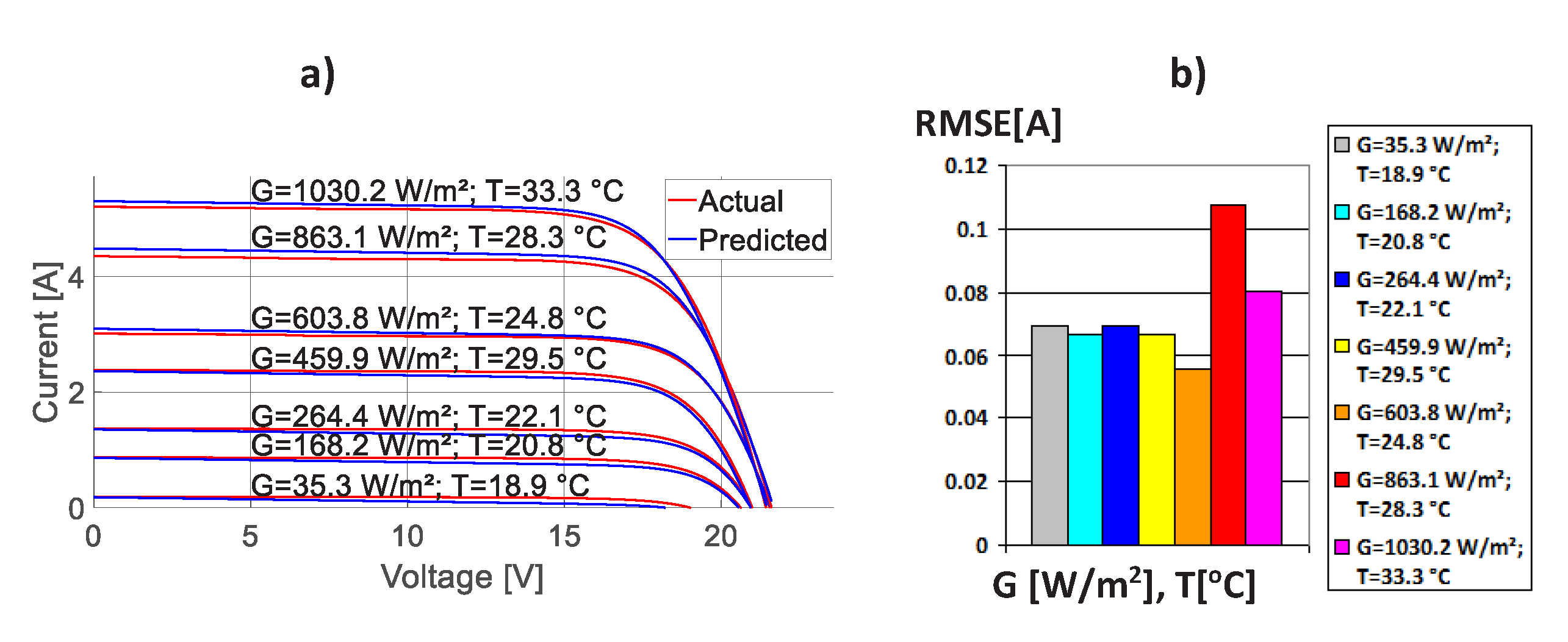
• Single-crystalline silicon PV panel
  As can be seen in Figure 7, for the single-crystalline silicon Cocoa xSi12922 PV panel, the predicted curves have high agreements with the actual curves. At high levels of solar irradiance and cell temperature (G = 603.8 $\mathrm{W}/{\mathrm{m}}^2$; T = 24.8 ${}^{°}\mathrm{C}$ to G = 1030.2 $\mathrm{W}/{\mathrm{m}}^2$; T = 33.3 ${}^{°}\mathrm{C}$), the proposal curves overestimate the output currents. On the other hand, at lower levels of solar irradiance and cell temperature (G = 35.3 $\mathrm{W}/{\mathrm{m}}^2$; T = 18.9 ${}^{°}\mathrm{C}$ to G = 459.9 $\mathrm{W}/{\mathrm{m}}^2$; T = 29.5 ${}^{°}\mathrm{C}$), the proposal curves underestimate the output currents.
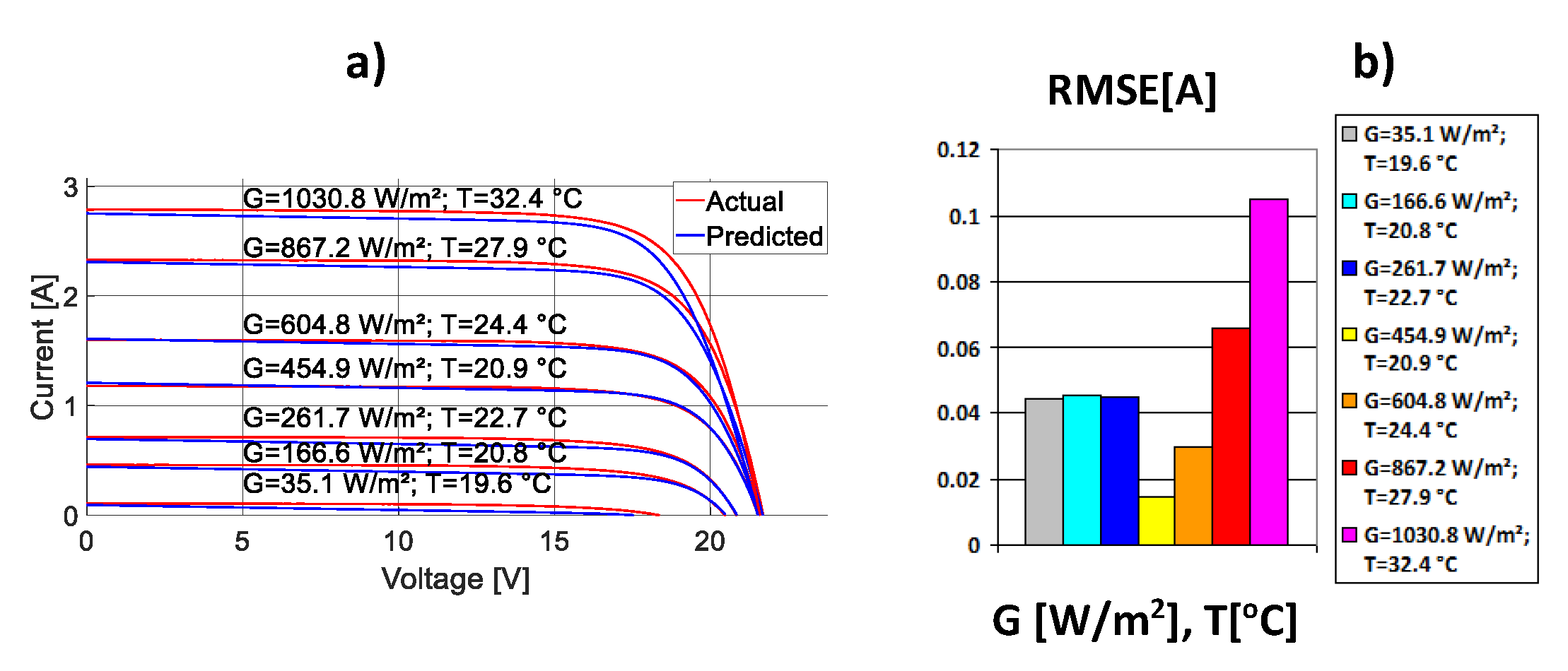
• Multi-crystalline silicon PV panel
  For the multi-crystalline silicon Cocoa mSi0166 PV panel in Figure 8, the model underestimates the current output. At low levels of solar irradiance and cell temperature, the disagreements between predicted curves and issued curves are larger, which can be explained by the uncertainties of experimental data tending to be bigger at low levels of T-G conditions. The predicted curves at high solar irradiance (867.2 $\mathrm{W}/{\mathrm{m}}^2$ and 1030.8 $\mathrm{W}/{\mathrm{m}}^2$) have inaccuracies with actual ones.
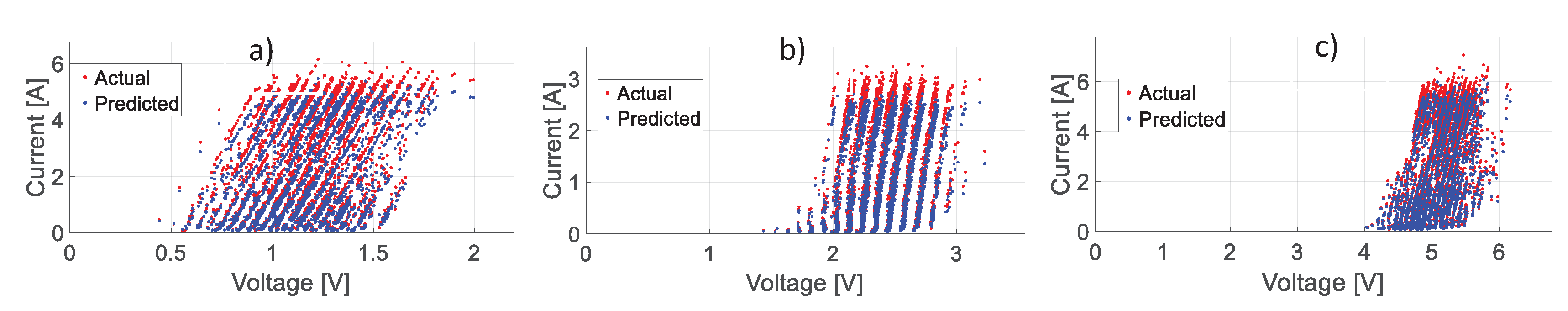
• HIT
  For the amorphous silicon (HIT) Cocoa HIT05667 PV panel in Figure 9, there are disagreements between estimated curves and issued curves; in particular, it tends to extend after the MPP.
  In Figure 7 and Figure 8, the RMSEs of the model are lowest at irradiances (400 $\mathrm{W}/{\mathrm{m}}^2$ to 600 $\mathrm{W}/{\mathrm{m}}^2$) and highest at 800 $\mathrm{W}/{\mathrm{m}}^2$ to 1000 $\mathrm{W}/{\mathrm{m}}^2$. There are two reasons for this tendency. The effectiveness of the SDM applying the proposed method is significantly affected by applying Equations (16) and (17). Consequently, in Figure 7, Figure 8 and Figure 9, the SDM shows more inaccuracies in open-circuit voltage. The RMSEs of the SDM at the solar irradiance from 30 $\mathrm{W}/{\mathrm{m}}^2$ to 270 $\mathrm{W}/{\mathrm{m}}^2$ is higher than the RMSEs of the SDM at the solar irradiance from 400 $\mathrm{W}/{\mathrm{m}}^2$ to 600 $\mathrm{W}/{\mathrm{m}}^2$ because the uncertainty of measuring instruments is higher when measuring at low levels of solar irradiance.
  As can be seen in Figure 9, the RMSEs are smaller at low levels of solar irradiance and cell temperature. The RMSEs tend to be higher at high levels of solar irradiance (635.1 $\mathrm{W}/{\mathrm{m}}^2$ to 1031.3 $\mathrm{W}/{\mathrm{m}}^2$) when they range from 0.2 to 0.3. At low levels of solar irradiance (35.5 $\mathrm{W}/{\mathrm{m}}^2$ to 1687 $\mathrm{W}/{\mathrm{m}}^2$) the RMSEs are lower with the RMSEs ranging from 0.05 to 0.1.
  The tendency of RMSEs in Figure 7 and Figure 8 is not as same as in Figure 9 because in the HIT PV panel, the fill factor is different from the two aforementioned PV types. The error of Equations (16) and (17) contributing to the SDM error surpasses the error of the uncertainty of measurement at low levels of solar irradiance.

In the above investigation, the model is tested by fixed levels of solar irradiance and cell temperature and various values of the external load, $R_L$. For given values of solar irradiance, cell temperature, and external load, the I-V characteristics of PV panels present the function $I=f\left(V\right)$ and the external load characteristic $I=V/R_L$ [17]. To make a more comprehensive validation, the proposed method is implemented for particular T-G conditions and constant values of the external load, which are characterized by 3000 pairs of ($T,G$). Figure 10 performs the predicted points and actual points for the Cocoa xSi12922 PV panel, the Cocoa mSi0166 PV panel, and the Cocoa HIT05667 PV panel, separately. The data show that the proposed method underestimates the output current for three types of panel. In addition, the simulation results tend to be more precise at lower values of T and G. The RMSE is 0.3544, 0.25, and 0.2888 for Cocoa xSi12922 PV panel, Cocoa mSi0166 PV panel, and Cocoa HIT05667 PV panel, respectively.

Four remarkable values, the open-circuit point voltage, the short-circuit current, the voltage, and current at the MPP, play the main role in obtaining the SDM as they provide the input for solving three main equations, Equations (6)–(8). In fact, expressions like Equations (16) and (17) cannot achieve the desired model precision. In addition, the coefficient of maximum power is not provided in the datasheets of some PV types; thus, the voltage and current at the MPP cannot be scaled. So, the SDM cannot be solved at other T-G conditions by the algorithm applied for solving the SDM at the STC; instead, a set of equations, Equations (61) and (65)–(68) are used to scale for each model parameter. This way might lead to the uncertainty of methods and reduce model accuracy.

7. Conclusions

In this article, seven methods of identifying parameters using the SDM have been reviewed and discussed comprehensively. The advantages and disadvantages of each method are analyzed. While some methods present good results in estimating the I-V curves in some cases, their reliability is not high when changing to other types of PV panels. A new method is proposed, which shows consistent performance for all investigated PV panels under various conditions of cell temperature and solar irradiance. This new method is verified in three types of PV panels, which are measured by NREL, USA. For three types of PV panels, single-crystalline silicon, multi-crystalline silicon, and amorphous silicon, the experimental results show RMSEs below 0.36. This error is an acceptable tolerance in practical applications requiring high accuracies such as PV power forecast and MPPT. Accurate I-V characteristics of PV panels contribute to the success in forecasting the maximum power point in the MPPT algorithm and the output power in PV power forecast.

References

- IEA. Tracking Power; IEA: Paris, France, 2019; Available online: https://www.iea.org/reports/trackingpower-2019 (accessed on 20 January 2020).
- IRENA. Future of Solar Photovoltaic: Deployment, Investment, Technology, Grid Integration and Socio-Economic Aspects (A Global Energy Transformation: Paper); International Renewable Energy Agency: Abu Dhabi, UAE, 2019. [Google Scholar]
- Bader, S.; Ma, X.; Oelmann, B. One-diode photovoltaic model parameters at indoor illumination levels—A comparison. Sol. Energy 2019, 180, 707–716. [Google Scholar] [CrossRef]
- El-Naggar, K.M.; AlRashidi, M.R.; AlHajri, M.F.; Al-Othman, A.K. Simulated Annealing algorithm for photovoltaic parameters identification. Sol. Energy 2012, 86, 266–274. [Google Scholar] [CrossRef]
- Krishnakumar, N.; Venugopalan, R.; Rajasekar, N. Bacterial foraging algorithm based parameter estimation of solar PV model. In Proceedings of the 2013 Annual International Conference on Emerging Research Areas and 2013 International Conference on Microelectronics, Communications and Renewable Energy, Kanjirapally, India, 4–6 June 2013. [Google Scholar]
- Zagrouba, M.; Sellami, A.; Bouaïcha, M.; Ksouri, M. Identification of PV solar cells and modules parameters using the genetic algorithms: Application to maximum power extraction. Sol. Energy 2010, 84, 860–866. [Google Scholar] [CrossRef]
- Ishaque, K.; Salam, Z. An improved modeling method to determine the model parameters of photovoltaic (PV) modules using differential evolution (DE). Sol. Energy 2011, 85, 2349–2359. [Google Scholar] [CrossRef]
- Khanna, V.; Das, B.K.; Bisht, D.; Singh, P.K. A three diode model for industrial solar cells and estimation of solar cell parameters using PSO algorithm. Renew. Energy 2015, 78, 105–113. [Google Scholar] [CrossRef]
- Oliva, D.; Cuevas, E.; Pajares, G. Parameter identification of solar cells using artificial bee colony optimization. Energy 2014, 72, 93–102. [Google Scholar] [CrossRef]
- Lin, P.; Cheng, S.; Yeh, W.; Chen, Z.; Wu, L. Parameters extraction of solar cell models using a modified simplified swarm optimization algorithm. Sol. Energy 2017, 144, 594–603. [Google Scholar] [CrossRef]
- Chen, Y.; Sun, Y.; Meng, Z. An improved explicit double-diode model of solar cells: Fitness verification and parameter extraction. Energy Convers. Manag. 2018, 169, 345–358. [Google Scholar] [CrossRef]
- De Blas, M.A.; Torres, J.L.; Prieto, E.; García, A. Selecting a suitable model for characterizing photovoltaic devices. Renew. Energy 2002, 25, 371–380. [Google Scholar] [CrossRef]
- Wang, G.; Zhao, K.; Shi, J.; Chen, W.; Zhang, H.; Yang, X.; Zhao, Y. An iterative approach for modeling photovoltaic modules without implicit equations. Appl. Energy 2017, 202, 189–198. [Google Scholar] [CrossRef]
- Femia, N.; Petrone, G.; Spagnuolo, G.; Vitelli, M. PV Modeling Power Electronics and Control Techniques for Maximum Energy Harvesting in Photovoltaic Systems; CRC Press: Boca Raton, FL, USA, 2017; pp. 1–33. [Google Scholar]
- Hussein, A. A simple approach to extract the unknown parameters of PV modules. Turkish J. Electr. Eng. Comput. Sci. 2017, 25, 4431–4444. [Google Scholar] [CrossRef]
- Celik, A.N.; Acikgoz, N. Modelling and experimental verification of the operating current of mono-crystalline photovoltaic modules using four- and five-parameter models. Appl. Energy 2007, 84, 1–15. [Google Scholar] [CrossRef]
- Lo Brano, V.; Orioli, A.; Ciulla, G.; Di Gangi, A. An improved five-parameter model for photovoltaic modules. Sol. Energy Mater. Sol. Cells 2010, 94, 1358–1370. [Google Scholar] [CrossRef]
- Gow, J.A.; Manning, C.D. Development of a photovoltaic array model for use in power-electronics simulation studies. IEE Proc. Electr. Power Appl. 1999, 146, 193–200. [Google Scholar] [CrossRef]
- Dehghanzadeh, A.; Farahani, G.; Maboodi, M. A novel approximate explicit double-diode model of solar cells for use in simulation studies. Renew. Energy 2017, 103, 468–477. [Google Scholar] [CrossRef]
- Wang, G.; Zhao, K.; Qiu, T.; Yang, X.; Zhang, Y.; Zhao, Y. The error analysis of the reverse saturation current of the diode in the modeling of photovoltaic modules. Energy 2016, 115, 478–485. [Google Scholar] [CrossRef]
- Arab, A.H.; Chenlo, F.; Benghanem, M. Loss-of-load probability of photovoltaic water pumping systems. Sol. Energy 2004, 76, 713–723. [Google Scholar] [CrossRef]
- Villalva, M.G.; Gazoli, J.R.; Filho, E.R. Comprehensive approach to modeling and simulation of photovoltaic arrays. IEEE Trans. Power Electron. 2009, 24, 1198–1208. [Google Scholar] [CrossRef]
- Cubas, J.; Pindado, S.; Victoria, M. On the analytical approach for modeling photovoltaic systems behavior. J. Power Sources 2014, 247, 467–474. [Google Scholar] [CrossRef]
- Ghani, F.; Duke, M. Numerical determination of parasitic resistances of a solar cell using the Lambert W-function. Sol. Energy 2011, 85, 2386–2394. [Google Scholar] [CrossRef]
- Jain, A.; Kapoor, A. Exact analytical solutions of the parameters of real solar cells using Lambert W-function. Sol. Energy Mater. Sol. Cells 2004, 81, 269–277. [Google Scholar] [CrossRef]
- Ghani, F.; Duke, M.; Carson, J. Numerical calculation of series and shunt resistances and diode quality factor of a photovoltaic cell using the Lambert W-function. Sol. Energy 2013, 91, 422–431. [Google Scholar] [CrossRef]
- Rusirawan, D.; Farkas, I. Identification of model parameters of the photovoltaic solar cells. Energy Procedia 2014, 57, 39–46. [Google Scholar] [CrossRef]
- De Soto, W.; Klein, S.A.; Beckman, W.A. Improvement and validation of a model for photovoltaic array performance. Sol. Energy 2006, 80, 78–88. [Google Scholar] [CrossRef]
- Walker, G. Evaluating MPPT converter topologies using a matlab PV model. J. Electr. Electron. Eng. 2001, 21, 49–55. [Google Scholar]
- Kennerud, K.L. Analysis of Performance Degradation in CDS Solar Cells. IEEE Trans. Aerosp. Electron. Syst. AES-5 1969, 6, 912–917. [Google Scholar] [CrossRef]
- Rodriguez, P.; Sera, D.; Teodorescu, R.; Rodriguez, P. PV Panel Model Based on Datasheet Values PV panel model based on datasheet values. In Proceedings of the IEEE International Symposium on Industrial Electronics, Vigo, Spain, 4–7 June 2007; pp. 2392–2396. [Google Scholar]
- Laudani, A.; Fulginei, F.R.; Salvini, A. Identification of the one-diode model for photovoltaic modules from datasheet values. Sol. Energy 2014, 108, 432–446. [Google Scholar] [CrossRef]
- Bana, S.; Saini, R.P. A mathematical modeling framework to evaluate the performance of single diode and double diode based SPV systems. Energy Rep. 2016, 2, 171–187. [Google Scholar] [CrossRef]
- Ciulla, G.; Lo Brano, V.; Di Dio, V.; Cipriani, G. A comparison of different one-diode models for the representation of I-V characteristic of a PV cell. Renew. Sustain. Energy Rev. 2014, 32, 684–696. [Google Scholar] [CrossRef]
- Humada, A.M.; Hojabri, M.; Mekhilef, S.; Hamada, H.M. Solar cell parameters extraction based on single and double-diode models: A review. Renew. Sustain. Energy Rev. 2016, 56, 494–509. [Google Scholar] [CrossRef]
- Marion, W.; Anderberg, A.; Deline, C.; Glick, S.; Muller, M.; Perrin, G.; Rodriguez, J.; Rummel, S.; Terwilliger, K.; Nrel, T.J.S. User’s Manual for Data for Validating Models for PV Module Performance. 2014. Available online: https://www.nrel.gov/docs/fy14osti/61610.pdf (accessed on 6 October 2019).