On the Applicability of Two Families of Cubic Techniques for Power Flow Analysis

Abstract

This work presents a comprehensive analysis of two cubic techniques for Power Flow (PF) studies. In this regard, the families of Weerakoon-like and Darvishi-like techniques are considered. Several theoretical findings are presented and posteriorly confirmed by multiple numerical results. Based on the obtained results, the Weerakoon’s technique is considered more reliable than the Newton-Raphson and Darvishi’s methods. As counterpart, it presents a high computational burden. Regarding this point, the Darvishi’s technique has turned out to be quite efficient and fully competitive with the Newton’s scheme.

1. Introduction

1.1. Motivation

In power system analysis, PF is probably the most important computational tool, playing a vital role in a wide variety of applications such as power system planning and operation, economic dispatch or security analysis, among others. From a mathematical point of view, PF consists on solving the set of equations that model the nonlinear relationships between nodal voltages and power injections. Since the PF equations are nonlinear, this problem cannot be directly solved. In this sense, iterative solvers have been customary used for solving the PF equations. From a PF solver one expects two main characteristics:

• Robustness: for effectively solving ill-conditioned systems, which are mainly encountered in presence of cascading failures, heavy loading conditions or badly initialization of the iterative procedure.
• Efficiency: this aspect is crucial for online applications, since it determines the ability of a PF solver for quickly finding the solution of the PF equations.

Many efforts have been devoted during decades on developing different PF solvers (see Literature Review). Developed approaches have been mainly focused on separately enhancing one of the characteristics enumerated above. However, in a modern power system paradigm, it is necessary to use tools that are simultaneously efficient and robust enough to, for example, properly handle large-scale ill-conditioned cases. In this context, it is very difficult to find a PF solver which gathers both robust and efficient features. For instance, the conventional Newton-Raphson (NR) can be considered an efficient technique, however, it fails in ill-conditioned systems being so its universal applicability questionable. Recently, some studies have been conducted on studying the applicability of various high-order Newton-like (HONL) methods for PF analysis [1,2,3,4], manifesting good performance in well-conditioned systems. However, these works lack of a formal analysis of the mathematical properties of such solvers, more specifically, their stability and robustness properties were not properly studied. This work aims at being a first step on filling this gap.

1.2. Literature Review

During decades, PF problem has been extensively investigated by the engineering community. In this context, the use of NR for PF solution at early 60’s [5] can be considered as one of the main milestones. By far, NR is nowadays the most widely employed solver in PF analysis, however, inversion or factorization of the Jacobian matrix supposed an important barrier for former computers. Thereby, many efforts were conducted on reducing this computational burden either by using decoupled techniques [6,7] or sparsity routines [8]. Decoupled techniques gained popularity during 80’s, nonetheless, the emergence of very efficient computational machines and the lack of effectiveness of such techniques in ill-conditioned systems limit their usage nowadays.

On the other hand, ill-conditioned systems began to be studied at 80’s due to the difficulty of the existing techniques to successfully solve such cases [9]. Firstly, ill-conditioning in power systems was most related with electric characteristics of the networks (i.e., high R/X ratio or heavy loading conditions). This definition has evolved towards being more related with the starting guess of the iterative procedure, according to the definition given in [10]. However, ill-conditioning in power systems is currently related with mathematical issues. During decades, solution of ill-conditioned PF problems has supposed as a main concern for engineering researchers. The very first steps in this direction [9] were devoted on developing robust techniques which resulted very inefficient in most cases (e.g., see results in [10]).

With the advent of 90’s, PF was revisited in order to address current issues. In this sense, PF analysis in distribution networks (radial or meshed) attracted huge attention. In this kind of networks, conventional (especially decoupled) solvers offered badly performance due to high R/X ratios or natural bad condition of such systems. To address such issues, huge efforts were conducted on developing specific solvers [11,12] and formulations [13,14,15]. However, this kind of techniques are very far to be considered universal methods as their main area of application lie in distribution systems. Actually, some of them cannot be directly applied in meshed networks [11]. In addition, some specific PF solvers such as the well-known backward-forward algorithm are totally inefficient in comparison with Newton-like methods (see results for radial networks in [3]).

Ill-conditioned systems were barely studied at the beginning of the 21st century, however, this issue have re-emerged in recent dates due to this kind of systems are becoming more frequent [16]. In addition, in contrast to the traditional ill-conditioned systems studied at 80’s which comprised very few buses [8], modern robust solvers require to be efficient and competitive with conventional techniques (e.g., NR) due to most of ill-conditioned cases are, in fact, very large (>1000 buses). In this sense, traditional robust approaches such like [9] can be considered totally out of date [10]. This way, multiple works have been recently conducted on developing efficient and robust techniques that could satisfactory addressed both well and ill-conditioned cases. The application of the Continuous Newton’s method for PF analysis [10,17,18,19] suppose a clear example of this trend. The Continuous Newton’s method establishes a formal analogy between NR and Euler’s techniques by which any other numerical integration method (e.g., the Runge-Kutta formulas [18]) could be applied for developing robust and efficient PF solvers. However, as reported in [18], those solvers based on the Continuous Newton’s method are still not competitive with NR in the sense that they are very inefficient. As a sake of example, the solver introduced in [10] which is based on the 4th order Runge-Kutta method requires four matrix factorizations. Since the factorization of the Jacobian matrix could be considered the heaviest computational part of a PF solver [10], one could deduce that the technique developed in [10] is four-times less efficient than NR. To address such issue, the authors developed a combined Runge-Kutta-Broyden paradigm in [20], which avoids the factorization of the Jacobian matrix. However, this calculation is replaced by the inversion of the Jacobian, which is unaffordable in large-scale systems. Similarly, the dynamic computing paradigm developed in [16] and its posterior refinements [21,22] are not suitable for large-scale cases, as the authors pointed out in [16].

Regularization-based methods have been recently applied for solving PF equations, especially in ill-conditioned cases [23,24]. This approach basically consists of avoiding the singularity of the Jacobian matrix when it is ill-conditioned, by adding the so-called regularizing operator. Due to the Jacobian matrix is modified, the solution of the iterative process may not be the actual solution of the PF problem, as commented in [24] and reported in [25]. This issue has limited the applicability of this kind of techniques. Homotopic and holomorphic principles have been also applied for solving PF problem [26,27]. This kind of methodologies solve the PF equations by posing a continuous version of them by which their solution is reaching by progressively increasing a well-known homotopic parameter. This kind of approaches are quite robust and have found certain interest on ill-conditioned cases. However, as in the case of regularization-based methods, they may reach a non-physical solution which lacks of interest [28]. Recently, the authors have developed various self-developed robust solvers [28,29], which arise from combination of different approaches. Although this kind of techniques present good computational performance, they are not competitive with other conventional techniques in well-conditioned cases yet.

Recently, HONL methods hav gained popularity for solving PF equations. Basically, a HONL is a nonlinear solved based on NR with a convergence order higher than two. Thus, a HONL should converge employing less iterations than NR. If besides this feature the solver is computationally efficient, the obtained PF solution approach may be competitive with NR. In this context, Pourbagher and Derakhshandeh firstly compared various HONL in [1], showed very good results. The conclusions in this reference motivated the authors to further study this kind of methods in [2,3,4], confirming that HONL methods may suppose an attractive alternative to NR.

1.3. Contributions and Paper Organization

Motivated by the good results showed by HONL techniques in recent studies. This work aims at further analyzing this kind of techniques for PF analysis. So far, HONL methods have been only employed for solving well-conditioned systems, therefore, their robust properties have not been analyzed from a theoretical and empirical point of view. This work aims at supposing a first step to filling this gap. In this sense, we focus on two well-known family of cubic techniques. In this context, we comprehensively analyze the cubic methods proposed by Weerakoon [30] (3OW) and Darvishi [31] (3OD). The stability, efficient and robustness properties of these solvers are firstly theoretically deduced and analyzed and, posteriorly, these theoretical foundations are empirically confirmed by numerical experiments. The two cubic methods are compared with the most standard PF solver (i.e., NR) and the 4th order Runge-Kutta method (RK4) developed in [10] with the aim of providing a benchmark study for the applicability of these families in both well and ill-conditioned systems. It is worth mentioning that these two cubic methodologies suppose the background for the development of many HONL techniques (e.g., see [32]). Thereby, this work aims at supposing a valuable guidance for applying other HONL techniques that are in fact modifications of the studied cubic techniques.

Remainder of this paper is organized as follows. Section 2 outlines the necessary background. Stability of two families of cubic techniques is studied in Section 3. Section 4 is devoted on comparing two families of cubic methods with the Newton-Raphson approach using a well-known efficiency index. Section 5 presents several numerical experiments with results. The main conclusions of this work are duly drawn in Section 6.

2. Background

2.1. PF Solution Using NR

In polar coordinates, the PF equations describe the nonlinear relationship between the nodal voltages and power injections. Thus, generically considering the $i^{th}$ system bus, the PF equations are given by [1,2,3,4]:

$$g\left(\mathit{x}\right)\left\{\begin{array}{c}{g}_{\mathit{P}}, \forall i\in \left[{\mathcal{N}}_l,{\mathcal{N}}_g\right]\\ g_{\mathit{Q}}, \forall i\in {\mathcal{N}}_l\end{array}\right.$$

(1)

$$g_{P_i}=P_i^{sch}-\sum \left|V_i\right|\left|V_j\right|\left|Y_{ij}\right|\cos \left({\theta }_{ij}-{\delta }_i+{\delta }_j\right)$$

(2)

$$g_{Q_i}=Q_i^{sch}-\sum \left|V_i\right|\left|V_j\right|\left|Y_{ij}\right|\sin \left({\theta }_{ij}-{\delta }_i+{\delta }_j\right)$$

(3)

$$\mathit{x}={\left[{\delta }_{\mathit{g}},{\delta }_{\mathit{l}},{\mathit{V}}_{\mathit{l}}\right]}^T$$

(4)

where, ${\mathcal{N}}_l$ and ${\mathcal{N}}_g$ are the sets of PQ and PV buses, respectively. $P_i^{sch}\in \mathcal{R}$ and $Q_i^{sch}\in ℝ$ are the active and reactive power injected at $i^{th}$ bus, respectively. $V_i\angle {\delta }_i\in ℂ$ is the complex voltage at $i^{th}$ bus. $Y_{ij}\angle {\theta }_{ij}\in ℂ$ is the $i{j}^{th}$ element of the admittance matrix, ${\delta }_g\in {ℝ}^{n_g}$ is the vector of voltage angles at PV buses, ${\delta }_{\mathit{l}}\in {ℝ}^{n_l}$ is the vector of voltage angles at PQ buses and $V_{\mathit{l}}\in {ℝ}^{n_l}$ is the vector of voltage angles at PQ buses, $n_l\in \mathbb{N}$ and $n_g\in \mathbb{N}$ are the total number of PQ buses and PV buses, respectively.

Because (1) are strongly nonlinear, they cannot be explicitly inverted. In PF analysis, iterative techniques are customary employed for addressing this issue and solving (1). Thereby, NR is often considered as the standard approach for PF purposes. PF solution using NR is established as a discrete map given by [2,3,4]:

$${\mathit{x}}_{k+1}={\mathit{x}}_k-{\left[g\prime \left({\mathit{x}}_k\right)\right]}^{-1}g\left({\mathit{x}}_k\right)$$

(5)

where $g^{\prime }={\nabla }_{\mathit{x}}g\in {ℝ}^{n\times n}$ is the Jacobian matrix and ${\left[·\right]}_k$ is the iteration counter. It is well-known that mapping (5) has quadratic order of convergence. Unlike to the mapping (5), HONL methods present order of convergence higher than two. In following Sections, we present two families of HONL techniques with third order of convergence.

2.2. Weerakoon-Like Methods for PF Analysis

Weerakoon and Fernando developed in [30] a nonlinear solver with cubic convergence rate (labelled 3OW in this work). Application of this technique to PF analysis leads to the following map:

$$\left\{\begin{array}{c}{\mathit{y}}_k={\mathit{x}}_k-{\left[g\prime \left({\mathit{x}}_k\right)\right]}^{-1}g\left({\mathit{x}}_k\right)\\ {\mathit{x}}_{k+1}={\mathit{x}}_k-2{\left[g\prime \left({\mathit{x}}_k\right)+g\prime \left({\mathit{y}}_k\right)\right]}^{-1}g\left({\mathit{x}}_k\right)\end{array}\right.$$

(6)

As observed, mapping (6) requires two Jacobian evaluations and two Lower-Upper (LU) decompositions. This approximately supposes doubling the computational cost of NR. Other nonlinear methodologies with cubic convergence rate based on mapping (6), have been developed and studied in [33,34,35,36].

2.3. Darvishi-Like Methods for PF Analysis

Darvishi and Barati studied a third order Newton-like technique in [31] (labelled by 3OD in this work). This approach was already applied to PF analysis in [1], leading to the following map:

$$\left\{\begin{array}{c}{\mathit{y}}_k={\mathit{x}}_k-{\left[g\prime \left({\mathit{x}}_k\right)\right]}^{-1}g\left({\mathit{x}}_k\right)\\ {\mathit{x}}_{k+1}={\mathit{y}}_k-{\left[g\prime \left({\mathit{x}}_k\right)\right]}^{-1}\left(g\left({\mathit{x}}_k\right)+g\left({\mathit{y}}_k\right)\right)\end{array}\right.$$

(7)

Alternatively, Babajee et al. [37] concluding in (7) by similitude with the Chebyshev’s method. 3OD responds to the structure of the so-called multipoint iterative methods [38]. These approaches achieve ${\left(N+1\right)}^{\mathrm{th}}$ order of convergence, where $N$ is the number of steps computed (two steps in (7)). In contrast to (5), the mapping (7) only requires a Lower-Upper (LU) factorization each iteration, however, the function $g$ has to be computed twice. For the sake of self-sufficiency, Figure 1 is a flowchart for PF solution using NR, 3OW or 3OD. As seen, the flowchart is the same for the three considered solvers. This evidences that the methods 3OW and 3OD are easily implementable in standard PF codes, thus only requiring minor modifications.

3. Stability of the Considered Cubic Methodologies

In order to study the stability of 3OW and 3OD, let us introduce the following definition:

Definition 1.

Hyperbolic points: a fixed point ${\mathit{x}}^{*}$of a map$G :C\subset {ℝ}^n\to {ℝ}^n$is hyperbolic, if the Jacobian of the equation $\dot{G}=G\left(\mathit{x}\right)-\mathit{x}$at${\mathit{x}}^{*}$has no eigenvalues with a zero real part. In addition, ${\mathit{x}}^{*}$is asymptotically stable if all the eigenvalues of the Jacobian of$\dot{G}$at${\mathit{x}}^{*}$have a modulus $\le 1$. A hyperbolic point can be:

• Sink: if all the eigenvalues of the Jacobian of $\dot{G}$ have a negative real part.
• Source: if at least one of the eigenvalues of the Jacobian of$\dot{G}$ has a positive real part.

In contrast, a fixed point is called unstable if it is not stable. 

The Definition 1 can be used to study the stability of an iterative map by assimilating it to a dynamic paradigm [10]. This way, one requires for a PF solution (namely ${\mathit{x}}^{*}$ such that $g\left({\mathit{x}}^{*}\right)=\mathbf{0}$) to be asymptotically stable. In addition, it is desirable that ${\mathit{x}}^{*}$ be a sink.

3.1. Stability of 3OW

In the case of mapping (6) one can write:

$$\dot{G}=-2{\left[g\prime \left(\mathit{x}\right)+g\prime \left(\mathit{y}\right)\right]}^{-1}g\left(\mathit{x}\right)$$

(8)

By differentiating (8) with respect $\mathit{x}$ one obtains:

$${\nabla }_{\mathit{x}}\dot{G}=-2\left({\nabla }_{\mathit{x}}{\left[g\prime \left(\mathit{x}\right)+g\prime \left(\mathit{y}\right)\right]}^{-1}g\left(\mathit{x}\right)+{\left[g\prime \left(\mathit{x}\right)+g\prime \left(\mathit{y}\right)\right]}^{-1}g\prime \left(\mathit{x}\right)\right)$$

(9)

On the other hand, by evaluating the first step of (6) at ${\mathit{x}}^{*}$ one obtains:

$${\left.\mathit{y}\right|}_{{\mathit{x}}^{*}}={\mathit{x}}^{*}-{\left[g\prime \left({\mathit{x}}^{*}\right)\right]}^{-1}g\left({\mathit{x}}^{*}\right)={\mathit{x}}^{*}$$

(10)

Then, evaluation of (9) at ${\mathit{x}}^{*}$ yields:

$${\left.{\nabla }_{\mathit{x}}\dot{G}\right|}_{{\mathit{x}}^{*}}=-2\left({\left[g\prime \left({\mathit{x}}^{*}\right)+g\prime \left({\mathit{x}}^{*}\right)\right]}^{-1}g\prime \left({\mathit{x}}^{*}\right)\right)=-2\left({\left[2g\prime \left({\mathit{x}}^{*}\right)\right]}^{-1}g\prime \left({\mathit{x}}^{*}\right)\right)=-\mathit{I}$$

(11)

where $\mathit{I}\in {ℝ}^{n\times n}$ is the identity operator. By (11), we can easily deduce that ${\mathit{x}}^{*}$ is asymptotically stable for the mapping (6). In addition, since all the eigenvalues of (11) have a negative real part, ${\mathit{x}}^{*}$ is also a sink for 3OW.

3.2. Stability of 3OD

For (7) one has that:

$$\dot{G}=-{\left[g\prime \left(\mathit{x}\right)\right]}^{-1}\left(g\left(\mathit{x}\right)+g\left(\mathit{y}\right)\right)$$

(12)

By differentiating (12) with respect $\mathit{x}$ one obtains:

$${\nabla }_{\mathit{x}}\dot{G}=-\left({\nabla }_{\mathit{x}}{\left[g\prime \left(\mathit{x}\right)\right]}^{-1}\left(g\left(\mathit{x}\right)+g\left(\mathit{y}\right)\right)+{\left[g\prime \left(\mathit{x}\right)\right]}^{-1}g\prime \left(\mathit{x}\right)+{\left[g\prime \left(\mathit{x}\right)\right]}^{-1}g\prime \left(\mathit{y}\right)\right)=-\left({\nabla }_{\mathit{x}}{\left[g\prime \left(\mathit{x}\right)\right]}^{-1}\left(g\left(\mathit{x}\right)+g\left(\mathit{y}\right)\right)+\mathit{I}+{\left[g\prime \left(\mathit{x}\right)\right]}^{-1}g\prime \left(\mathit{y}\right)\right)$$

(13)

As observed, equation (10) is also valid for the mapping (7). Consequently, one could write:

$${\left.{\nabla }_{\mathit{x}}\dot{G}\right|}_{{\mathit{x}}^{*}}=-\left({\nabla }_{\mathit{x}}{\left[g\prime \left({\mathit{x}}^{*}\right)\right]}^{-1}\left(0+g\left({\left.\mathit{y}\right|}_{{\mathit{x}}^{*}}\right)\right)+\mathit{I}+{\left[g\prime \left({\mathit{x}}^{*}\right)\right]}^{-1}g\prime \left({\left.\mathit{y}\right|}_{{\mathit{x}}^{*}}\right)\right)=-\left(\mathit{I}+{\left[g^{\prime }\left({\mathit{x}}^{*}\right)\right]}^{-1}{g}^{\prime }\left({\mathit{x}}^{*}\right)\right)=-2\mathit{I}$$

(14)

As checked by (14), ${\mathit{x}}^{*}$ is a sink for the mapping (7), however, it is not asymptotically stable. From the results obtained in this Section, it is concluded that the Weerakoon-like techniques are more stable than the Darvishi-like approaches.

4. A Comparison of the Considered Cubic Techniques

Table 1. Main computations involved in PF solution using NR, 3OW and 3OD.

Computation	PF Solution Method
	NR (5)	3OW (6)	3OD (7)
Function evaluations ($K_1$)	1	1	2
Jacobian evaluations ($K_2$)	1	2	1
Factorizations ($n_{LU}$)	1	2	1
Linear systems solved ($q$)	1	2	2

summarizes the main computations involved in an iteration of the mappings (5)–(7).

From Table 1 may look that the Newton-Raphson technique is the most efficient mapping. However, the order of convergence should be also taken into account. In order to properly consider this aspect, let us introduce the following efficiency index [39]:

$$\mu =p^{\raisebox{1ex}{$1$}\!\left/ \!\raisebox{-1ex}{$CO$}\right.}$$

(15)

where, $p\in {ℝ}^{+}$ is the order of convergence and $CO$ stands for the total computational cost of an iteration in terms of flops. In this regards, the cost of a LU decomposition may be estimated using the following Theorem.

Theorem 1.

The number of products and quotients required for solving $q$ linear systems of equations with the same matrix of coefficients, by using LU factorization, is:

$$o\left(n,q\right)=\frac{1}{3}{n}^3+q{n}^2-\frac{1}{3}n$$

(16)

The proof of the Theorem 1 can be found in [40].

Finally, by considering the cost of each function $o\left(g\right)=n$ and Jacobian evaluation $o\left(g^{\prime }\right)=n^2$, the total computational cost of an iteration might be expressed as follows:

$$CO=K_{1}o\left(g\right)+K_{2}o\left(g^{\prime }\right)+{{\displaystyle \sum }}_{m=1}^{m=n_{LU}}o\left(n,q_m\right)$$

(17)

where $K_1\in \mathbb{N}$ is the number of function evaluations, $K_2\in \mathbb{N}$ is the number of Jacobian evaluations, $n_{\mathrm{LU}}$ is the number of LU factorizations and $q_m$ indicates how many linear systems are solved using the $m^{th}$ LU factorization. The value of these parameters for each studied solver were summarized in Table 1. With this information, the following Theorems are devoted on estimating the total computational cost of the maps (6) and (7), respectively.

Theorem 2.

Computational cost of 3OW: for the mapping (3), one has $\mu =3^{\raisebox{1ex}{$1$}\!\left/ \!\raisebox{-1ex}{$\frac{2}{3}{n}^3+4n^2+\frac{1}{3}n$}\right.}$.

Proof of the Theorem 2.

From Table 1 we have that $K_1=1$, $K_2=2$ and $K_3=2$. On the other hand, each LU decomposition is devoted on solving a linear system, therefore, $q=1$ for both LU decompositions. Finally, it is well-known that $p=3$ for mapping (6) (a proof is provided in [30]). Thus:

$$CO=n+2n^2+2\left(\frac{1}{3}{n}^3+n^2-\frac{1}{3}n\right)=\frac{2}{3}{n}^3+4n^2+\frac{1}{3}n$$

(18)

Therefore:

$$\mu =3^{\raisebox{1ex}{$1$}\!\left/ \!\raisebox{-1ex}{$\frac{2}{3}{n}^3+4n^2-\frac{1}{3}n$}\right.}$$

(19)

which completes the proof. □

Theorem 3.

Computational cost of 3OD: for the mapping (7), one has $\mu =3^{\raisebox{1ex}{$1$}\!\left/ \!\raisebox{-1ex}{$\frac{1}{3}{n}^3+3n^2+\frac{5}{3}n$}\right.}$.

Proof of the Theorem 3.

From Table 1 we have that $K_1=2$, $K_2=1$ and $K_3=1$. On the other hand, the LU decomposition is devoted on solving two linear systems, therefore, $q=2$. Finally, it is well-known that $p=3$ for mapping (7) (a proof is provided in [31] and [37]). Thus:

$$CO=2n+n^2+\frac{1}{3}{n}^3+n^2-\frac{1}{3}n=\frac{1}{3}{n}^3+3n^2+\frac{5}{3}n$$

(20)

Therefore:

$$\mu =3^{\raisebox{1ex}{$1$}\!\left/ \!\raisebox{-1ex}{$\frac{1}{3}{n}^3+3n^2+\frac{5}{3}n$}\right.}$$

(21)

which completes the proof. □

The results of the Theorems 2 and 3 allow to compare the methods 3OW and 3OD with NR. In this sense, Figure 2 plots the value of (12) for the mappings (5)–(7). Clearly, 3OD is the most efficient solver, which was expected since this technique only requires one LU factorization but achieves cubic convergence. In contrast, 3OW lower efficiency index than NR. This low degree of efficiency is undoubtedly due to the extra LU factorization in comparison with (5) and (7). One should note that, especially in large systems, the factorization of the Jacobian matrix is the heaviest part of any PF calculation [10].

5. Numerical Experiments

This Section is devoted on presenting some numerical results, which aim to illustrate the advantages and disadvantages of the considered cubic methods in PF studies. For this purpose, the considered families of cubic methods are compared with the conventional NR and the PF solver based on the 4th order Runge-Kutta (RK4) developed in [10]. Throughout this Section, the following cases will be considered:

• The IEEE 30-, and 300-bus test systems [41,42].
• The 1354-, 2869-, and 9241-bus portions of the European Transmission System from the EU Pegase Project [43,44].
• The 2736-bus snapshot of the Polish Transmission System at summer 2004 peak [45].

For the sake of self-sufficiency,

Table 2. Main characteristics of the studied systems.

System	Buses	Branches	Generators	Load		$\mathit{n}$
				MW	MVar
30-bus	30	41	6	283.4	126.2	53
300-bus	300	411	69	23,525.8	7788.0	530
1354-bus	1354	1991	260	73,059.7	13,401.4	2447
2736-bus	2736	3504	420	18,074.5	5339.5	5237
2869-bus	2869	4582	510	132,437.3	29,007.8	5227
9241-bus	9241	16,049	1445	312,354.1	73,581.6	17,036

summarizes the main characteristics of the studied systems. Along NR and RK4 in polar coordinates, the iterative procedures defined by (6) and (7) have been coded in Matpower [46]. In all cases, $g{\left(\mathit{x}\right)}_{\infty }<{10}^{-6}$ has been imposed as convergence criterion. The accuracy of the different techniques has been compared with the so-established correct solution of each system (calculated by using NR and the initial point defined in Matpower), concluding that solution achieved by all the considered solvers in the case studies are in essence the same operational point. In this sense, all considered techniques have been concluded to be accurate enough and a further comparative analysis have not been included as it lacks of importance.

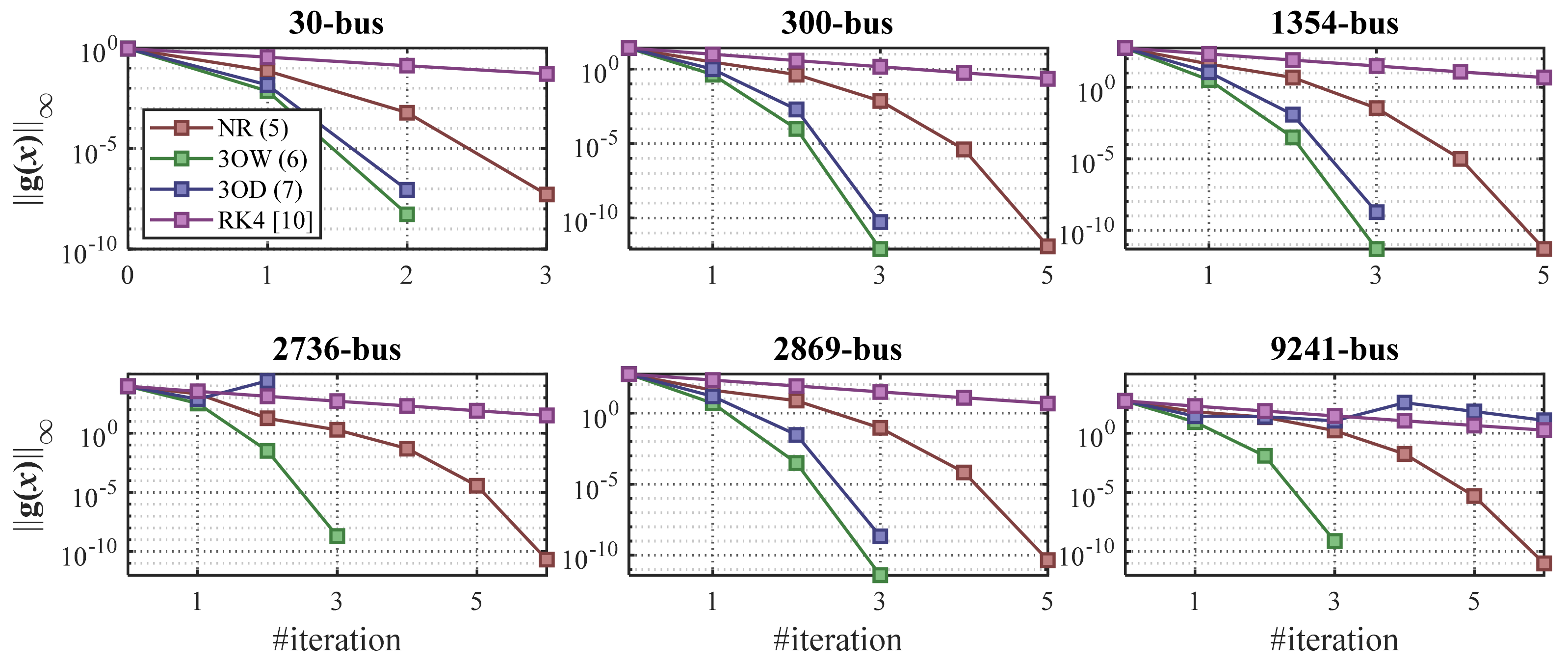
5.1. Convergence Rates

The first test is focused on comparing the convergence rates showed by the considered methods. A priori, one can guess that 3OW and 3OD solvers will exhibit higher convergence rate than NR and RK4 due to their cubic convergence features. However, a deeper comparison among 3OW and 3OD techniques has to be empirically carried out. Thereby, Figure 3 plots the convergence profiles for the studied systems. As expected, the cubic techniques required less iterations than NR and RK4. On the other hand, 3OW clearly exhibited the highest convergence rate. It is worth mentioning that 3OD failed in the 2736-, and 9241-bus cases, which confirms, to some extent, the conclusions drawn in Section 3.

5.2. Solution Times

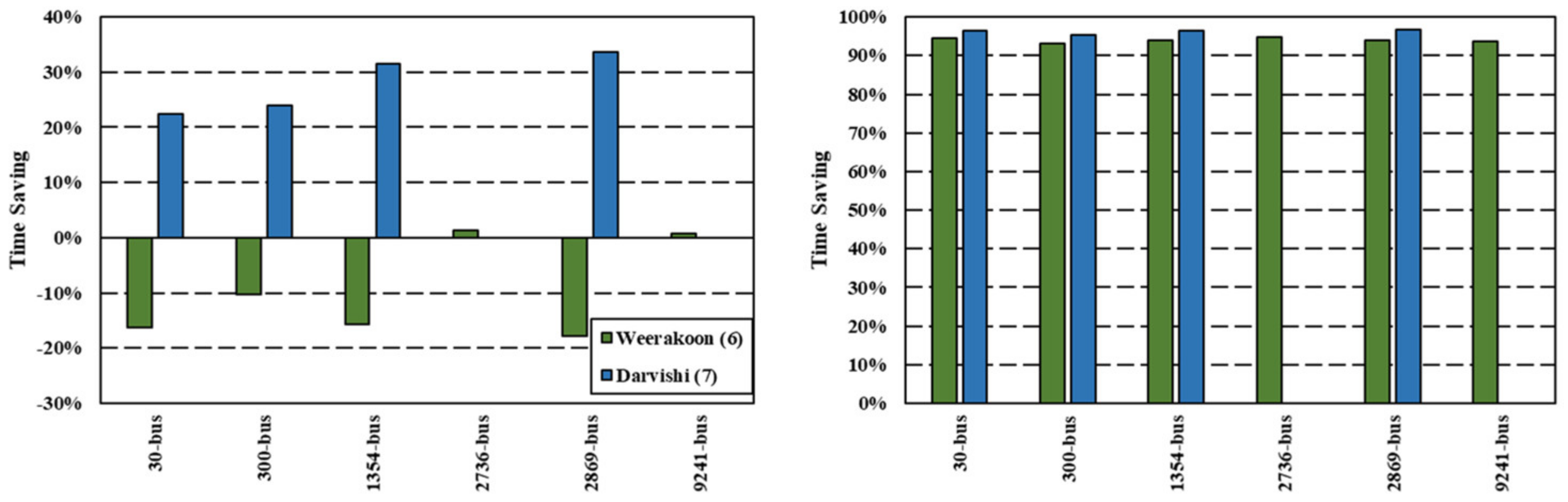
Now, the efficiency of the different studied solvers is analyzed. To do that, solution times employed by the different techniques for solving the cases studies are compared.

Table 3. Solution times [ms].

System	NR (5)	RK4 (10)	3OW (6)	3OD (7)
30-bus	3.30	70.50	3.84	2.56
300-bus	11.48	185.26	12.66	8.72
1354-bus	41.55	797.22	48.07	28.42
2736-bus	100.69	1902.75	99.35
2869-bus	93.91	1860.29	110.59	62.38
9241-bus	387.29	6052.44	384.23

reports the solution times in milliseconds, required by the studied techniques. These results have been obtained on a 64-bit i5-9400F Intel Core personal computer (2.90 GHz, 8 GB of RAM). In order to avoid the influence of other computational activities, the reported results have been calculated as the average values of 100 simulations. As observed, 3OD was clearly the most efficient technique (even more than NR). Nevertheless, we have to remark that this algorithm failed in the 2736-, and 9241-bus systems. On the other hand, 3OW resulted not competitive w.r.t. NR as it normally takes longer solution times. To get a better overview, Figure 4 provides a comparison of the computational saving offered by 3OW and 3OD w.r.t. NR and RK4. As seen, while 3OD was able to improve by ~30% the results obtained with NR, 3OW was usually inefficient in comparison with the mapping (5). As expected, computational superior of cubic techniques is more noticeable in comparison with RK4, because this solver requires 4 LU factorizations per iteration and presents a very low convergence rate. These results empirically confirm the conclusions drawn in the efficiency analysis performed in Section 4.

The reason behind the low degree of efficiency of the mapping (6), lies in the fact that it requires two LU factorizations each iteration. As commented, the factorization of the Jacobian matrix may be considered as the heaviest part of any PF calculation, due to its computational cost is $o\left(n^3\right)$. As checked in

Table 4. Total LU Factorizations.

System	NR (5)	RK4 (10)	3OW (6)	3OD (7)
30-bus	3	64	4	2
300-bus	5	80	6	3
1354-bus	5	96	6	3
2736-bus	6	112	6
2869-bus	5	96	6	3
9241-bus	6	96	6

, 3OW often required more LU decompositions than the remainder techniques. At the same time, one can check that 3OD typically computed less factorizations than NR and RK4, which explains why this technique resulted competitive compared with NR.

5.3. Influence of the Loading Level

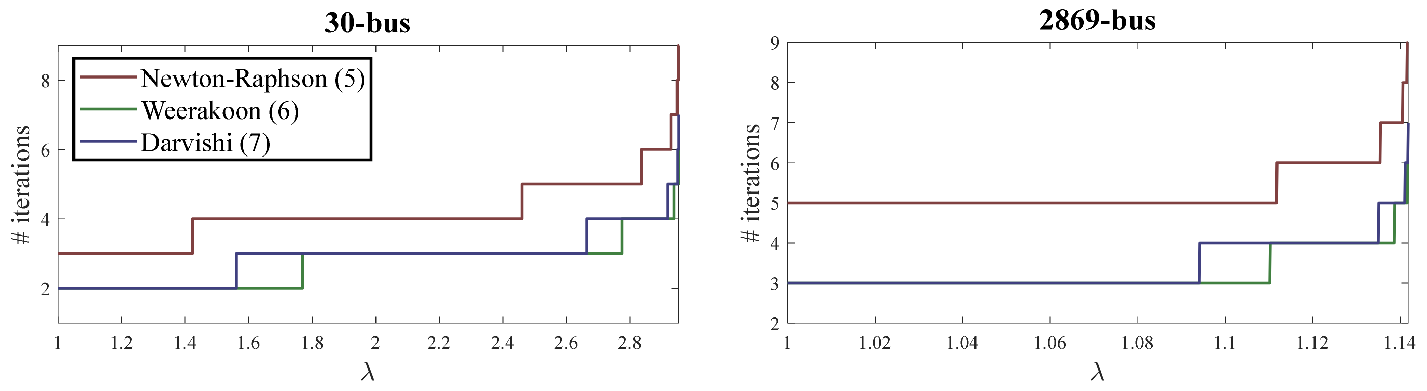
Next, les us examine the influence of the loading level in the overall performance of the studied algorithms. To do that, we have modified the power profiles of the studied systems as follows:

$$P_i^{sch}=\lambda P_i^{sch}, \mathrm{for}\mathrm{all}\mathrm{buses}$$

(22)

$$Q_i^{sch}=\lambda Q_i^{sch}, \mathrm{for}\mathrm{PQ}\mathrm{buses}$$

(23)

where $\lambda \in {ℝ}^{+}$ is the loading level. Figure 5 shows the total number of iterations required by the different studied solvers for different loading levels. For the sake of simplicity, only results in in the 30-, and 2869-bus systems have been reported, since similar conclusions were observed by the authors in the other cases. As expected, 3OW and 3OD outperformed NR in all studied systems. It is worth observing that 3OW is less affected by the loading level than 3OD. Results for RK4 are not shown in Figure 5 for facilitating its visualization (note that this technique employed many iterations even for solving the base case).

5.4. Contractive Properties

Next, we aim to check the contractive properties of the analyzed mappings. Firstly, it is suitable to present the following Theorem:

Theorem 4.

Contraction map Theorem: Let ${\mathit{x}}^{*}$ be a root of the mapping $G$. If there exists a neighbourhood $S\left({\mathit{x}}^{*},\delta \right)$ and a positive constant $\eta \in \left(0,1\right)$ such that $‖G\left(\mathit{x}\right)-G\left({\mathit{x}}^{*}\right)‖\le \eta ‖\mathit{x}-{\mathit{x}}^{*}‖$, then the sequence ${\left\{{\mathit{x}}_k\right\}}_{k=0}^{\infty }$ defined by ${\mathit{x}}_{k+1}=G\left({\mathit{x}}_k\right)$ converges to ${\mathit{x}}^{*}$ for any ${\mathit{x}}_0\subset S$.

Proof of the Theorem 4 can be found in [47]. Theorem 4 provides sufficient (but not necessary) conditions for convergence. Here, two aspects deserve to be remarked:

• Convergence of a mapping is ensured if the following

  $$\eta =\frac{‖G\left(\mathit{x}\right)-G\left({\mathit{x}}^{*}\right)‖}{‖\mathit{x}-{\mathit{x}}^{*}‖}<1$$

  (24)

  holds.
• Intuitively, one can guess that the lowest $\eta$ the highest degree of robustness and stability.

This way, one can analyse the contractive properties (and indirectly the stability and robustness features) of an iterative mapping by observing the value of $\eta$. This analysis has been performed for the studied solvers in various cases studies and the results are shown in Figure 6 plots the value of $\eta$ for NR, RK4, 3OW and 3OD in the 30-, 2736-, and 9241-bus cases. In this case, the point ${\mathit{x}}^{*}$ has been calculated using the Newton-Raphson technique with the initial guess provided in Matpower with convergence tolerance equals to ${10}^{-9}$. From Figure 6 it is clearly observed that 3OW presents better contractive properties than the other solvers. Indeed, in the 2736-, and 9241-bus systems the ratio $\eta$ is occasionally greater than one for NR and 3OD, while the relation (24) holds in all cases when 3OW is used. In the case of RK4, it still present good contractive properties due to the condition (24) holds in all studied cases, however, the ratio $\eta$ decreased very slowly due to this solver presents a very low convergence rate.

5.5. Influence of the Initial Guess

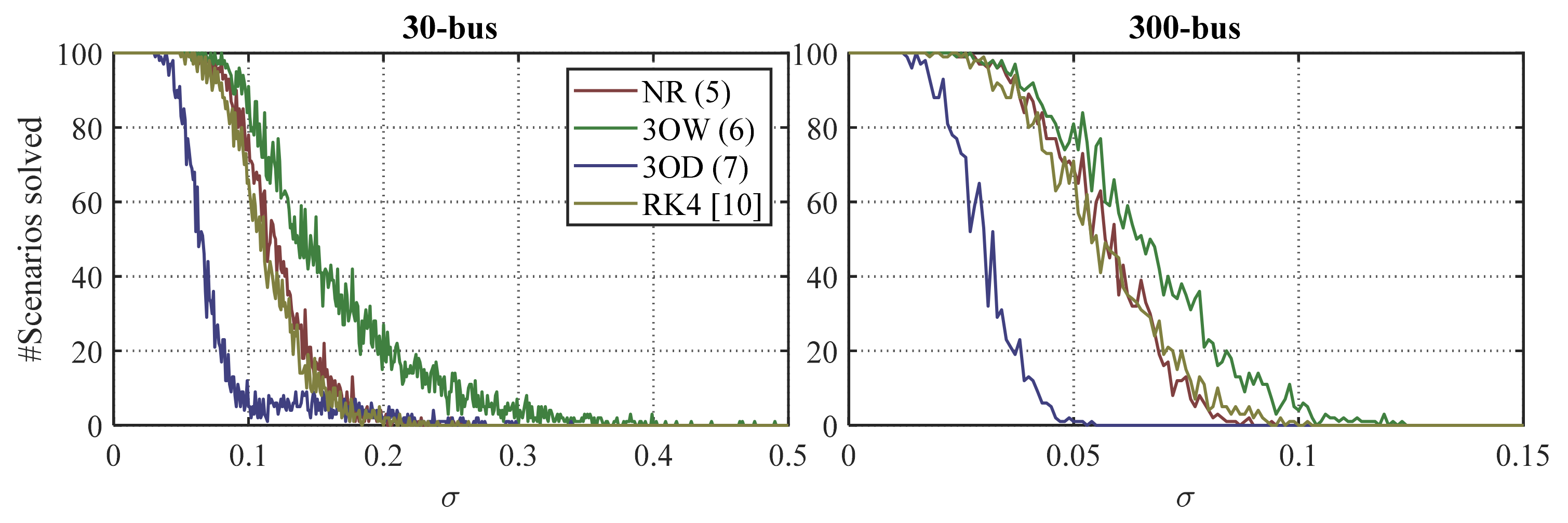
It is well-known that NR has local convergence [47]. This entails that successful convergence of this algorithm is strongly influenced by the initial guess ${\mathit{x}}_0$. Generally, one can affirm that the mapping (5) converges if ${\mathit{x}}_0$ lies sufficiently close to ${\mathit{x}}^{*}$. However, since ${\mathit{x}}^{*}$ is normally unknown, choosing a suitable ${\mathit{x}}_0$ might be a critical task. In this Section we aim to discern if the considered cubic techniques are wider or narrower convergent that NR technique. To do that, we have performed a statistical analysis, which a set of different initial guesses is built as follows:

$${\mathit{x}}_0~\mathcal{N}\left({\mathit{x}}^{*},\sigma \right)$$

(25)

where $\mathcal{N}\left({\mathit{x}}^{*},\sigma \right)$ is a Gaussian distribution with mean ${\mathit{x}}^{*}$ and standard deviation $\sigma$. We have considered up to 100 different initial guesses for different standard deviations. Figure 7 plots the total number of scenarios successfully solved by different methods, in the 30-, and 300-bus cases. As observed, NR and RK4 presented similar performance and were outperformed by 3OW, which resulted to be the less sensitive method. In contrast, 3OD has turned out to be scarcely reliable.

To complete the Section, we have considered the ill-posed versions of the 1345-, 2869- and 9241-bus cases, which can be found in [48]. These cases present an initial point for which NR fails to converge. Thereby, considering the definition provided in [10], these cases can be considered ill-conditioned. In order to provide a better overview in such systems, we have included RK4 (10) in the analysis, since this solver could be considered robust. Figure 8 shows the convergence profiles in these cases. As observed, while NR typically showed an oscillatory pattern 3OD diverged in all the studied cases, 3OW was successful in all the studied cases. These results strengthen the ideas outlined in Section 3. It is worth remarking that, despite RK4 could be considered a robust solver, it failed in the 2869- and 9241-bus cases. Finally, comparison of the computational burden between RK4 and 3OW is addressed in

Table 5. Solution times [ms] in the ill-conditioned version of the 1354-bus system.

Method	Total	Iteration
3OW (6)	40.15	8.03
RK4 (10)	804.26	33.51

for the ill-posed version of the 1354-bus case. As seen, RK4 consumed much more time than 3OW. A further insight allows to compare the average time consumed in each iteration of both techniques. As observed, the computational burden of RK4 is much higher than that observed for 3OW, which is expected as the RK4 requires up to four LU factorizations each iteration.

6. Concluding Remarks

This work has presented a comprehensive analysis of two families of HONL techniques, in order to validate them for PF studies. This analysis has been supported on theoretical findings and numerical results.

This way, The Weerakoon (3OW) and Darvishi (3OD) families of cubic techniques have been considered, since they suppose the main background for developing multiple HONL approaches. This way, this work aims at serving as valuable benchmark for developing and applying other multiple HONL techniques for PF analysis in the future.

The first block of this manuscript has developed various theoretical findings on the basis of well-known theorems. This analysis has yielded as main conclusion that 3OW is more stable but less efficient than 3OD.

In a second part, various numerical experiments have been performed to confirm the theoretical findings encountered in the previous study. In these experiments, the considered cubic methods have been compared with the well-known NR and RK4 techniques. The results reported allow to assert that 3OW generally result to be more robust and presents better convergence rate compared with NR and 3OD. In addition, this technique seems to be less affected by the loading level and the initial guess. The main drawback of 3OW is its low degree of efficiency. In this aspect, it has been usually outperformed by the 3OD, which has turned out to be very efficient (even more than NR). However, 3OD has resulted very weak and totally not suitable for ill-conditioned systems.

On the light of the results obtained, we believe that the Weerakoon-like techniques may be fully competitive with the Newton’s scheme, due to their intrinsic robust features. In this regard, future works should be focused on reducing its computational burden by proposing alternative schemes.

References

- Pourbagher, R.; Derakhshandeh, S.Y. Application of high-order newton-like methods to solve power flow equations. IET Gener. Transm. Distrib. 2016, 10, 1853–1859. [Google Scholar] [CrossRef]
- Tostado, M.; Kamel, S.; Jurado, F. Developed Newton-Raphson based predictor-corrector load flow approach with high convergence rate. Int. J. Electric. Power Energy Syst. 2019, 105, 785–792. [Google Scholar] [CrossRef]
- Tostado-Véliz, M.; Kamel, S.; Jurado, F. A novel family of efficient power-flow methods with high convergence rate suitable for large realistic power systems. IEEE Syst. J. 2021, 15, 738–746. [Google Scholar] [CrossRef]
- Tostado-Véliz, M.; Kamel, S.; Jurado, F. Two efficient and reliable power-flow methods with seventh order of convergence. IEEE Syst. J. 2021, 15, 1026–1035. [Google Scholar] [CrossRef]
- Tinney, W.F.; Hart, C.E. Power flow solution by Newton’s method. IEEE Trans. Power Appar. Syst. 1967, PAS-86, 1449–1460. [Google Scholar] [CrossRef]
- Wang, L.; Lin, X.R. Robust fast decoupled power flow. IEEE Trans. Power Syst. 2000, 15, 208–215. [Google Scholar] [CrossRef]
- Dasgupta, K.; Swarup, K.S. Distributed fast decoupled load flow analysis. In 2008 Joint International Conference on Power System Technology and IEEE Power India Conference; IEEE: New Delhi, India, 2008; pp. 1–6. [Google Scholar] [CrossRef]
- Gnanavignesh, R.; Shenoy, U.J. Parallel sparse LU factorization of power flow jacobian using GPU. In TENCON 2019—2019 IEEE Region. 10 Conference (TENCON); IEEE: Piscataway, NJ, USA, 2019; pp. 1857–1862. [Google Scholar] [CrossRef]
- Iwamoto, S.; Tamura, Y. A load flow calculation method for ill-conditioned power systems. IEEE Trans. Power Appar. Syst. 1981, PAS-100, 1736–1743. [Google Scholar] [CrossRef]
- Milano, F. Continuous newton’s method for power flow analysis. IEEE Trans. Power Syst. 2009, 24, 50–57. [Google Scholar] [CrossRef]
- Kersting, W.H. Distribution System Modeling and Analysis, 2nd ed.; CRC Press: Boca Raton, FL, USA, 2006. [Google Scholar]
- Farivar, M.; Low, S.H. Branch flow model: Relaxations and convexification-part I. IEEE Trans. Power Syst. 2013, 28, 2554–2564. [Google Scholar] [CrossRef]
- Kamel, S.; Abdel-Akher, M.; Jurado, F. Improved NR current injection load flow using power mismatch representation of PV bus. Int. J. Electr. Power Energy Syst. 2013, 53, 64–68. [Google Scholar] [CrossRef]
- Penido, D.R.R.; de Araujo, L.R.; Júnior, S.C.; Pereira, J.L.R. A new tool for multiphase electrical systems analysis based on current injection method. Int. J. Electr. Power Energy Syst. 2013, 44, 410–420. [Google Scholar] [CrossRef]
- Saleh, S.A. The formulation of a power flow using d-q reference frame components-part II: Unbalanced 3φ systems. IEEE Trans. Ind. Appl. 2018, 54, 1092–1107. [Google Scholar] [CrossRef]
- Xie, N.; Torelli, F.; Bompard, E.; Vaccaro, A. Dynamic computing paradigm for comprehensive power flow analysis. IET Gener. Transm. Distrib. 2013, 7, 832–842. [Google Scholar] [CrossRef]
- Tostado-Véliz, M.; Kamel, S.; Jurado, F. Development of different load flow methods for solving large-scale ill-conditioned systems. Int. Trans. Electr. Energy Syst. 2019, 29, e2784. [Google Scholar] [CrossRef]
- Tostado-Véliz, M.; Kamel, S.; Jurado, F. Comparison of various robust and efficient load-flow techniques based on Runge–Kutta formulas. Electr. Power Syst. Res. 2019, 174, 105881. [Google Scholar] [CrossRef]
- Tostado-Véliz, M.; Kamel, S.; Jurado, F. A robust power flow algorithm based on bulirsch–stoer method. IEEE Trans. Power Syst. 2019, 34, 3081–3089. [Google Scholar] [CrossRef]
- Tostado-Véliz, M.; Kamel, S.; Jurado, F. Development of combined Runge-Kutta Broyden’s load flow approach for well and ill-conditioned power systems. IET Gener. Transm. Distrib. 2018, 12, 5723–5729. [Google Scholar] [CrossRef]
- Xie, N.; Bompard, E.; Napoli, R.; Torelli, F. Widely convergent method for finding solutions of simultaneous nonlinear equations. Electr. Power Syst. Res. 2012, 83, 9–18. [Google Scholar] [CrossRef]
- Torelli, F.; Vaccaro, A. A second order dynamic power flow model. Electr. Power Syst. Res. 2013, 126, 12–20. [Google Scholar] [CrossRef]
- Milano, F. Analogy and convergence of Levenberg’s and Lyapunov-based methods for power flow analysis. IEEE Trans. Power Syst. 2016, 31, 1663–1664. [Google Scholar] [CrossRef]
- Tostado, M.; Kamel, S.; Jurado, F. An effective load-flow approach based on Gauss-Newton formulation. Int. J. Electr. Power Energy Syst. 2019, 113, 573–581. [Google Scholar] [CrossRef]
- Tostado-Véliz, M.; Kamel, S.; Jurado, F. An efficient and reliable power flow solution method for large scale Ill-Conditioned cases based on the Romberg’s integration scheme. Int. J. Electr. Power Energy Syst. 2020, 123, 106264. [Google Scholar] [CrossRef]
- Mehta, D.; Nguyen, H.D.; Turitsyn, K. Numerical polynomial homotopy continuation method to locate all the power flow solutions. IET Gener. Transm. Distrib. 2016, 10, 2972–2980. [Google Scholar] [CrossRef] [Green Version]
- Feng, Y.; Tylavsky, D.J. A Holomorphic embedding approach for finding the Type-1 power-flow solutions. Int. J. Electr. Power Energy Syst. 2019, 102, 179–188. [Google Scholar] [CrossRef]
- Karimi, M.; Shahriari, A.; Aghamohammadi, M.R.; Marzooghi, H.; Terzija, V. Application of Newton-based load flow methods for determining steady-state condition of well and ill-conditioned power systems: A review. Int. J. Electr. Power Energy Syst. 2019, 113, 298–309. [Google Scholar] [CrossRef]
- Tostado-Véliz, M.; Kamel, S.; Jurado, F. An efficient power-flow approach based on Heun and King-Werner’s methods for solving both well and ill-conditioned cases. Int. J. Electr. Power Energy Syst. 2020, 119, 105869. [Google Scholar] [CrossRef]
- Weerakoon, S.; Fernando, T.G.I. A variant of Newton’s method with accelerated third-order convergence. Appl. Math. Lett. 2000, 13, 87–93. [Google Scholar] [CrossRef]
- Darvishi, M.T.; Barati, A. A third-order Newton-type method to solve systems of nonlinear equations. Appl. Math. Comput. 2007, 187, 630–635. [Google Scholar] [CrossRef]
- Chun, C.; Neta, B. Developing high order methods for the solution of systems of nonlinear equations. Appl. Math. Comput. 2019, 342, 178–190. [Google Scholar] [CrossRef]
- Frontini, M.; Sormani, E. Some variant of Newton’s method with third-order convergence. Appl. Math. Comput. 2003, 140, 419–426. [Google Scholar] [CrossRef]
- Özban, A.Y. Some new variants of Newton’s method. Appl. Math. Lett. 2004, 17, 677–682. [Google Scholar] [CrossRef] [Green Version]
- Frontini, M.; Sormani, E. Third-order methods from quadrature formulae for solving systems of nonlinear equations. Appl. Math. Comput. 2004, 149, 771–782. [Google Scholar] [CrossRef]
- Cordero, A.; Torregrosa, J.R. Variants of Newton’s method for functions of several variables. Appl. Math. Comput. 2006, 183, 199–208. [Google Scholar] [CrossRef]
- Babajee, D.K.R.; Dauhoo, M.Z.; Darvishi, M.T.; Karami, A.; Barati, A. Analysis of two Chebyshev-like third order methods free from second derivatives for solving systems of nonlinear equations. J. Comput. Appl. Math. 2010, 233, 2002–2012. [Google Scholar] [CrossRef] [Green Version]
- Traub, J.F. Iterative Methods for the Solution of Equations, 2nd ed.; American Mathematical Society: New York, NY, USA, 1982. [Google Scholar]
- Lotfi, T.; Bakhtiari, P.; Cordero, A.; Mahdiani, K.; Torregrosa, J.R. Some new efficient multipoint iterative methods for solving nonlinear systems of equations. Int. J. Comput. Math. 2015, 92, 1921–1934. [Google Scholar] [CrossRef] [Green Version]
- Cordero, A.; Hueso, J.L.; Martínez, E.; Torregrosa, J.R. A modified Newton-Jarratt’s composition. Numer. Algorithms 2010, 5, 87–99. [Google Scholar] [CrossRef]
- Birchfield, A.B.; Xu, T.; Gegner, K.M.; Shetye, K.S.; Overbye, T.J. Grid structural characteristics as validation criteria for synthetic networks. IEEE Trans. Power Syst. 2017, 32, 3258–3265. [Google Scholar] [CrossRef]
- Peyghami, S.; Davari, P.; Fotuhi-Firuzabad, M.; Blaabjerg, F. Standard test systems for modern power system analysis: An overview. IEEE Ind. Electron. Mag. 2019, 13, 86–105. [Google Scholar] [CrossRef]
- Fliscounakis, S.; Panciatici, P.; Capitanescu, F.; Wehenkel, L. Contingency ranking with respect to overloads in very large power systems taking into account uncertainty, preventive, and corrective actions. IEEE Trans. Power Syst. 2013, 28, 4909–4917. [Google Scholar] [CrossRef] [Green Version]
- Josz, C.; Fliscounakis, S.; Maeght, J.; Panciatici, P. AC power flow data in MATPOWER and QCQP format: ITesla, RTE snapshots, and PEGASE. arXiv 2016, arXiv:1603.01533. Available online: http://arxiv.org/abs/1603.01533 (accessed on 22 June 2021).
- MATPOWER. Available online: http://www.pserc.cornell.edu/matpower/ (accessed on 22 June 2021).
- Zimmerman, R.D.; Murillo-Sánchez, C.E.; Thomas, R.J. MATPOWER: Steady-state operations, planning, and analysis tools for power systems research and education. IEEE Trans. Power Syst. 2011, 26, 12–19. [Google Scholar] [CrossRef] [Green Version]
- Ortega, J.M.; Rheinboldt, W.C. Iterative Solution of Nonlinear Equations in Several Variables; Society of Industrial Applied Mathematics: Philadelphia, PA, USA, 2000. [Google Scholar]
- Modified EU Pegase Systems. Available online: https://zenodo.org/record/3553615 (accessed on 22 June 2021).
Figure 1.
Flowchart for the application of NR, 3OW or 3OD for PF analysis.
Figure 2.
Efficiency index (15) for the considered mappings.
Figure 3.
Convergence profiles in the studied cases.
Figure 4.
Time savings of 3OW and 3OD w.r.t. NR (left) and RK4 (right).
Figure 5.
Total iterations for different loading levels.
Figure 6.
Value of the ratio in different cases using various solvers.
Figure 7.
Total scenarios successfully solved by NR, 3OW and 3OD using different initial guesses.
Figure 8.
Convergence profiles in the modified EU Pegase systems.