High-Accuracy Power Quality Disturbance Classification Using the Adaptive ABC-PSO as Optimal Feature Selection Algorithm

Abstract

Power quality disturbance (PQD) is an important issue in electrical distribution systems that needs to be detected promptly and identified to prevent the degradation of system reliability. This work proposes a PQD classification using a novel algorithm, comprised of the artificial bee colony (ABC) and the particle swarm optimization (PSO) algorithms, called “adaptive ABC-PSO” as the feature selection algorithm. The proposed adaptive technique is applied to a combination of ABC and PSO algorithms, and then used as the feature selection algorithm. A discrete wavelet transform is used as the feature extraction method, and a probabilistic neural network is used as the classifier. We found that the highest classification accuracy (99.31%) could be achieved through nine optimally selected features out of all 72 extracted features. Moreover, the proposed PQD classification system demonstrated high performance in a noisy environment, as well as the real distribution system. When comparing the presented PQD classification system’s performance to previous studies, PQD classification accuracy using adaptive ABC-PSO as the optimal feature selection algorithm is considered to be at a high-range scale; therefore, the adaptive ABC-PSO algorithm can be used to classify the PQD in a practical electrical distribution system.

1. Introduction

The demand for electricity in Thailand has continually increased over the past several decades, due mainly to an expansion of industrial and commercial customers. Numerous load types have been installed to the grid according to the various customer types [1,2,3]. The power quality disturbance (PQD) is an important issue in electrical distribution systems, especially since this issue becomes more severe in a system having different load types [4]. PQD can significantly decrease the reliability and performance of the grid [5,6]. According to international standards, i.e., EN 50160 and IEEE-1159, PQD can occur in various forms, such as voltage sag, flicker, swell, harmonic distortion, momentary interruption, spike, notch, transient, or a combination of these forms [7,8,9]. The power quality signals are generally categorized into stationary and nonstationary signals, which can be characterized and analyzed either by time-domain or frequency domain analysis methods [10].

Feature extraction is a well-known and reliable procedure used to identify performance degradation in a distribution system caused by PQD; feature selection and feature classifiers are also useful [11]. Feature extraction is a signal processing method to estimate the signals’ data based on its statistics [11]. So far, several signal processing tools have been used for feature extraction, depending on the type of signals [12]. The empirical mode decomposition (EMD) is one of the signal analysis methods for time-domain analysis; meanwhile, Fourier transform (FT) is extensively used in the frequency domain signal analysis [13]. The wavelet transform (WT) and S-transform (ST) are applicable for both time and frequency domain signal analysis [14,15,16], and their outstanding ability makes them a suitable signal analysis method for feature selection. FT is usually used for characterizing the spectrum and harmonics of the stationary signal, whereas it is inappropriate to identify the characteristics of nonstationary signals, due to its fixed window function [10,17]. The short-time Fourier transform (STFT) was used to improve the time–frequency window of the FT during the temporary, transient signal localization [18]. ST has been proposed to improve the localization of the STFT [19]; nevertheless, ST still has poor detection potentiality for nonstationary transient disturbances [20]. The Discrete Wavelet Transform (DWT) was developed from the STFT to improve the fixed resolution issue; this extraction method can provide a short window in high-frequency compositions while maintaining a long window at low-frequency components. In the literature, DWT has been widely used for signal detection and feature extraction of a transient disturbance, i.e., fault detection and identification of the transmission line, PQD classification, and islanding detection [21,22,23].

Since feature extraction is insufficient to classify the type of power quality signals accurately, an additional tool called a “classifier” is used after the feature extraction process to improve the accuracy of power quality signal identification [10]. Artificial intelligence (AI) is widely known as an effective tool used to identify the power quality signals and solve many problems in power systems research [24,25,26]. AI is an automatic system that can behave similarly to human thinking, and can engage in decision-making, learning, problem-solving, perception, reasoning, and classification [12,27]. In particular, several AI techniques, i.e., Expert Systems, Fuzzy Logic, Artificial neural networks, and Genetic Algorithms (GA), have been applied to PQD classification, showing that it could precisely classify the power quality signal type [28,29,30,31,32,33,34]. The neural network especially demonstrates higher performance at classifying the PQD than many other AI techniques [35,36,37].

In addition, the feature selection process has been implemented extensively to increasingly improve the precision of PQD identification [38,39,40]. Feature selection is the process that eliminates the redundant information of the feature extracting data, aiming to improve accuracy and reduce the computational time of the PQD classification. Several previous studies have demonstrated that PQD classification adopting feature selection can achieve high accuracy. In 2009, adaptive particle swarm optimization (PSO) was proposed as the optimal feature selection algorithm for PQD classification, based on ST feature extraction to identify nine PQD types; this classification system could provide 96.33% accuracy [37]. H. Erişti et al. presented the k-means with the Apriori algorithm to determine the optimal feature of PQD classification using five PQD signals, and it was shown that an accuracy of 98.88% could be reached [36]. After that, the PQD classification system based on the PSO algorithm as the optimal feature selection algorithm with DWT feature extraction was introduced by R. Ahila et al. [41]. This system could provide a classification accuracy of 97.60% for ten PQD signals. A. A. Abdoos et al. showed that their PQD classification system using the Sequential Forward Selection (SFS) algorithm to find the optimal features could achieve up to 99.66% classification accuracy [13]. In 2018, the Fisher linear discriminant analysis (FDA) algorithm was performed as the optimal feature selection to classify the 15 PQD types based on Variational Mode Decomposition (VMD) as feature extraction, indicating that an accuracy of 98.82% could be accomplished [39]. Recently, L. Fu et al. performed Permutation Entropy with the Fisher Score algorithm to find the optimal feature based on 13 PQD types [40]. It was found that this system has an accuracy of 97.6%.

From the previous studies, we noticed that the PQD classification system’s performance could be improved increasingly. In this paper, a combination of the adaptive artificial bee colony (ABC) and the PSO algorithms is introduced and applied to identify 13 PQD signals. We propose a high-accuracy PQD classification using a novel algorithm called “adaptive ABC-PSO” as the feature selection algorithm. The inspiration for this proposed feature selection algorithm was implementing the merit of PSO to compensate for ABC’s weakness; the adaptive technique was also applied to improve the combination algorithm’s searching ability. The feature extraction of the presented classification system was based on the DWT, whereas the probabilistic neural network (PNN) was performed as the classifier.

2. Power Quality Disturbances

In this work, 13 types of power quality signals were used for PQD classification. Ten single types of PQD signals were the pure sine waveform, sag, swell, interruption, harmonics, impulsive transients, oscillatory transients, flicker, notch, and spikes, whereas the rest were multiple-type PQD signals, including sag with harmonics, swell with harmonics, and interruption with harmonics. The mathematical models for PQD signal generation were based on the IEEE-1159 standard, as shown in

Table 1. Mathematical equations of power quality disturbances (PQDs) [7].

Label	Disturbance Class	Mathematic Modeling Equation	Parameter Constraints
C1	Pure sine	$y(t)=A\sin (\omega t)$	$A=1$
C2	Sag	$y(t)=A[1-\alpha (u(t-t_1)-u(t-t_1))]\sin (\omega t)$	$0.1\le \alpha \le 0.9; T\le t_2-t_1\le 9T$
C3	Swell	$y(t)=A[1+\alpha (u(t-t_1)-u(t-t_1))]\sin (\omega t)$	$0.1\le \alpha \le 0.8; T\le t_2-t_1\le 9T$
C4	Interruption	$y(t)=A[1-\alpha (u(t-t_1)-u(t-t_1))]\sin (\omega t)$	$0.9\le \alpha \le 1; T\le t_2-t_1\le 9T$
C5	Harmonic	$y(t)=A[{\alpha }_1\sin (\omega t)+{\alpha }_3\sin (3\omega t)+{\alpha }_5\sin (5\omega t)+{\alpha }_7\sin (7\omega t)]$	$0.05\le {\alpha }_3,{\alpha }_5,{\alpha }_7\le 0.15; {\displaystyle \sum {\alpha }_i^2=1}$
C6	Impulsive transient	$y(t)=A[1-\alpha \{u(t-t_1)-u(t-t_1)\}]\sin (\omega t)$	$\begin{array}{l}0\le {\alpha }_i\le 0.414; \\ T/20\le t_2-t_1\le T/10\end{array}$
C7	Oscillatory transient	$y(t)=A[\sin (\omega t)+{\alpha }^{-c(t-t_1)/\tau }\sin {(\omega t)}_n(t-t_1)(u(t_2)-u(t_1))]$	$\begin{array}{l}0.1\le \alpha \le 0.8; 0.5T\le t_2-t_1\le 3T;\\ 8\le \tau \le 40ms; 300\le f_n\le 900Hz\end{array}$
C8	Flicker	$y(t)=A[1+{\alpha }_f\sin (\beta \omega t)]\sin (\omega t)$	$0.1\le {\alpha }_f\le 0.2; 5\le \beta \le 20Hz$
C9	Notch	$\begin{array}{l}y(t)=\sin (\omega t)-sign(\sin (\omega t))\\ \times \left\{{\displaystyle {\sum }_{n=0}^{9}K\times \left[u\left(t-\left(t_1-0.02n\right)\right)-u\left(t-\left(t_2-0.02n\right)\right)\right]}\right\}\end{array}$	$\begin{array}{l}0\le t_1,t_2\le 0.5T;\\ 0.01T\le t_2-t_1\le 0.005T; \\ 0.1\le K\le 0.4\end{array}$
C10	Spikes	$\begin{array}{l}y(t)=\sin (\omega t)-sign(\sin (\omega t))\\ \times \left\{{\displaystyle {\sum }_{n=0}^{9}K\times \left[u\left(t-\left(t_1-0.02n\right)\right)-u\left(t-\left(t_2-0.02n\right)\right)\right]}\right\}\end{array}$	$\begin{array}{l}0\le t_1,t_2\le 0.5T;\\ 0.01T\le t_2-t_1\le 0.005T;\\ 0.1\le K\le 0.4\end{array}$
C11	Sag with harmonic	$\begin{array}{l}y(t)=A[1-\alpha (u(t-t_1)-u(t-t_1))]\\ [{\alpha }_1\sin (\omega t)+{\alpha }_3\sin (3\omega t)+{\alpha }_5\sin (5\omega t)+{\alpha }_7\sin (7\omega t)]\end{array}$	$\begin{array}{l}0.1\le \alpha \le 0.9; T\le t_2-t_1\le 9T;\\ 0.05\le {\alpha }_3,{\alpha }_5,{\alpha }_7\le 0.15; {\displaystyle \sum {\alpha }_i^2=1}\end{array}$
C12	Swell with harmonic	$\begin{array}{l}y(t)=A[1+\alpha (u(t-t_1)-u(t-t_1))]\\ [{\alpha }_1\sin (\omega t)+{\alpha }_3\sin (3\omega t)+{\alpha }_5\sin (5\omega t)+{\alpha }_7\sin (7\omega t)]\end{array}$	$\begin{array}{l}0.1\le \alpha \le 0.8; T\le t_2-t_1\le 9T;\\ 0.05\le {\alpha }_3,{\alpha }_5,{\alpha }_7\le 0.15; {\displaystyle \sum {\alpha }_i^2=1}\end{array}$
C13	Interruption with harmonic	$\begin{array}{l}y(t)=A[1-\alpha (u(t-t_1)-u(t-t_1))]\\ [{\alpha }_1\sin (\omega t)+{\alpha }_3\sin (3\omega t)+{\alpha }_5\sin (5\omega t)+{\alpha }_7\sin (7\omega t)]\end{array}$	$\begin{array}{l}0.9\le \alpha \le 1; T\le t_2-t_1\le 9T;\\ 0.05\le {\alpha }_3,{\alpha }_5,{\alpha }_7\le 0.15; {\displaystyle \sum {\alpha }_i^2=1}\end{array}$

. All PQD waveforms were considered for 10 cycles with 2000 sampling points, signal amplitude of 1 p.u., electrical frequency of 50 Hz, and sampling frequency of 10 kHz. The signals were randomly generated for each test within their mathematical constraints.

3. Feature Extraction

Feature extraction is the process of initializing the group of datasets as features by reducing raw data. Figure 1 shows that the dataset of power quality signals is passed through the WT with multi-resolution analysis (MRA) to obtain signals’ wavelet coefficients. The statistical parameters of signals are calculated by the obtained coefficients and used for feature vector construction. This section is organized as follows: Section 3.1 describes the wavelet transform. Then, the MRA and the feature vector construction are explained in Section 3.2 and Section 3.3, respectively.

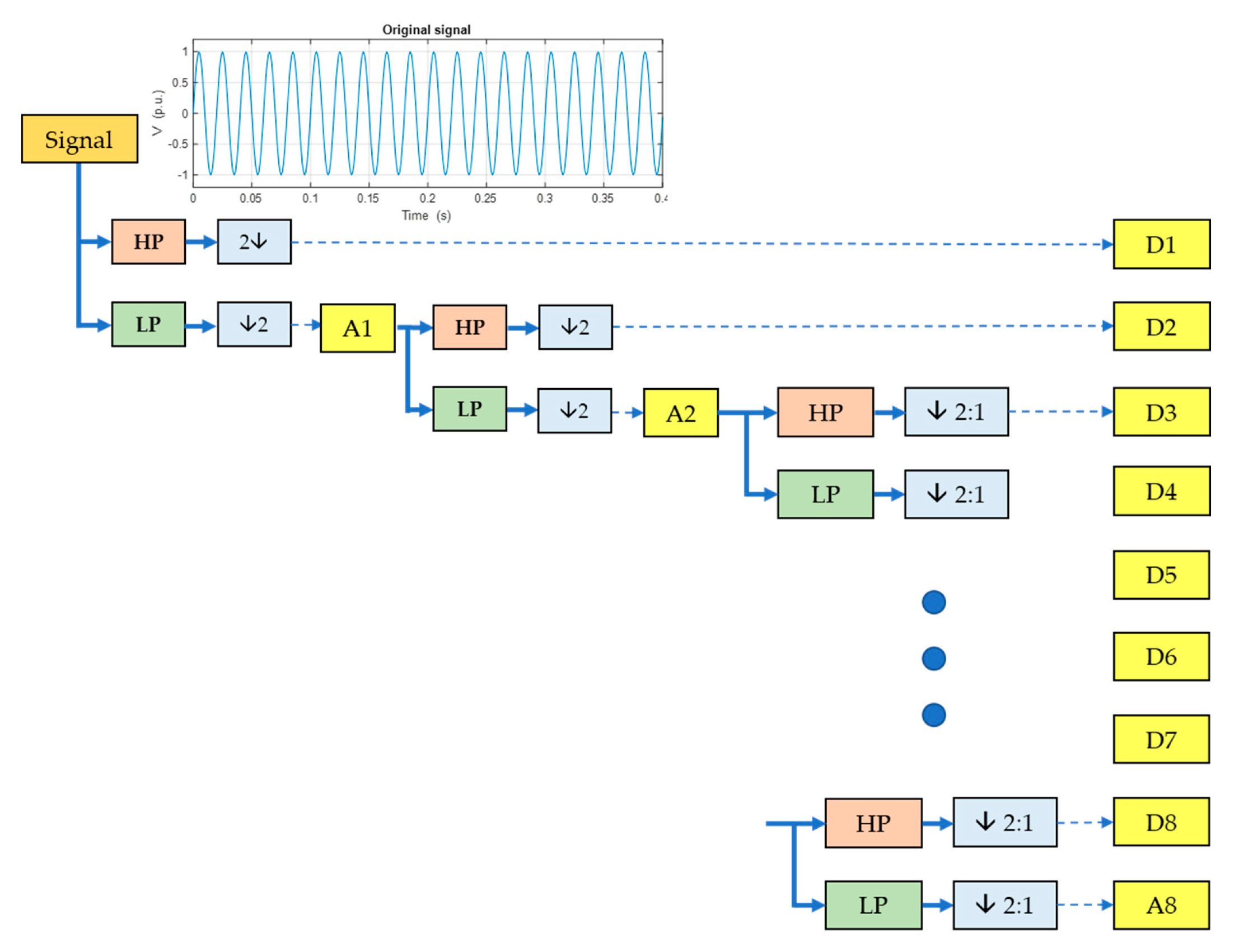
3.1. Wavelet Transform

In power quality research, the WT and ST are widely known as efficient signal processing techniques. The WT is a signal processing tool that can identify the global and local components of signals through the wavelet function. The advantages of WT are its resilient time-scale representation and good conservation of time and frequency information without resolution reduction compared to the STFT; however, the WT sometimes requires complicated setting parameters. The ST is extended from the continuous wavelet transform, which magnifies the referenced phase information in specific frequency bands with suitable expanse and contraction of Gaussian window as the mother wavelet. Comparing the WT to the ST shows that the WT indicates a simpler implementation and requires less memory storage than ST; therefore, the WT is more suitable for the PQD classification of numerous signal types [21,22,23,42]. In this work, we performed WT in PQD classification, since the number of signal types is huge (13 types). The DWT is developed from the WT using a discrete set of wavelet scales. This method has been extensively performed to detect the characteristics of signals, especially in the feature extraction of the recent PQD classification research [21]. In this work, we performed the DWT to identify the characteristics of signals in the feature extraction process. The expression for DWT can be written as Equation (1).

$$DWT(m,n)=\frac{1}{\sqrt{a_0^m}}{\displaystyle \sum _{k}f(k)}\psi \left(\frac{(n-k{b}_0{a}_0^m)}{a_0^m}\right)$$

(1)

where $a_0^m$ is the scaling parameter representing the recurrence and the length of wavelet as a function of the indicated frequency localization, $m$. $b_0$ is the translation parameter that collects a moving position of wavelet. The parameter $n$ indicates the time localization. $f(k)$ is the sequence of discrete point of continuous-time. The $\psi$ is called the mother wavelet. In this paper, the fourth-order Daubechies (dB4) was used as the mother wavelet, since it was claimed in many studies that this value is suitable for analysis of power system transient signals and power quality signals [23,43,44,45].

3.2. Multi-Resolution Analysis

The theory of the MRA algorithm was introduced by S. G. Mallat in 1989 [44]. This algorithm uses the scaling function and the orthogonal wavelet function to decompose and reconstruct signals at different resolution levels. The decomposition of a time-varying signal, $f(t)$, can be written in terms of the scaling, ${\phi }_{m,n}$, and the wavelet, ${\psi }_{m,n}$, as shown in Equations (2) and (3), respectively.

$${\phi }_{m,n}=2^{\left(-\frac{m}{2}\right)}\phi \left(2^{-m}t-n\right)$$

(2)

$${\psi }_{m,n}=2^{\left(-\frac{m}{2}\right)}\psi \left(2^{-m}t-n\right)$$

(3)

Figure 2 shows that the time-varying signal is passed through a system consisting of Low-Pass (LP) and High-Pass (HP) filters at each resolution level. After the original time-domain signal is passed through the HP filter and downsampling afterwards, the high-frequency components with the first detail coefficient signal ($D_1$) are obtained. Similarly, the low-frequency component with the first approximation coefficient signal, ($A_1$), is obtained after LP filtering and the original signal’s downsampling. After that, the output of signal ($A_1$) is decomposed to produce the second detail coefficient signal ($D_2$) and ($A_2$). This procedure was performed repeatedly until the desired decomposition level was obtained. In this work, the decomposition level was set to be eight levels, since this value results in the appropriate frequency range of each decomposed level for characterizing the disturbances of the focused power quality signals [18]. Then, the feature vector of the PDQ signals, $F(k)$, can be written as Equation (4).

$$F(k)=[ \begin{array}{ccccccccc}{D}_1& D_2& D_3& D_4& D_5& D_6& D_7& D_8& A_8\end{array}]$$

(4)

3.3. Feature Vector Construction

When the PQD signals are passed to the MRA process, nine signal characteristics are obtained through the statistical parameters’ signal features. In this work, the eight features included the energy ($E$), entropy ($Ent$), standard deviation ($\sigma$), mean value ($\mu$), kurtosis ($KT$), skewness ($SK$), root-mean square ($RMS$), and range ($RG$). The statistical equation for each feature is given in

Table 2. Statistical parameter equations.

Parameter	Statistical Equation	Parameter	Statistical Equation
Energy	$E_i={\displaystyle {\sum }_{j=1}^N\left({\left|X_{lj}\right|}^2\right)}$	Kurtosis	$K{T}_i=\frac{E{(X_{lj}-{\mu }_l)}^4}{{\sigma }_l^4}$
Entropy	$En{t}_i=-{\displaystyle {\sum }_{j=1}^N\left\{X_{lj}^2\log X_{lj}^2\right\}}$	Skewness	$S{K}_i=\frac{E{(X_{lj}-{\mu }_l)}^3}{{\sigma }_l^3}$
Standard deviation (S.D.)	${\sigma }_i={\left(\frac{1}{n-1}{\displaystyle {\sum }_{j=1}^N\left\{{\left(X_{lj}-{\mu }_l\right)}^2\right\}}\right)}^{\frac{1}{2}}$	RMS	$RM{S}_i={\left(\frac{1}{n}{\displaystyle {\sum }_{j=1}^N{\left(X_{lj}\right)}^2}\right)}^{\frac{1}{2}}$
Mean	${\mu }_i=\frac{1}{n}{\displaystyle {\sum }_{j=1}^N\left(X_{lj}\right)}$	Range	$R{G}_i=Max\left(X_{lj}\right)-Min\left(X_{lj}\right)$

, where $i, j$ = 1, 2, 3, …, $l$ are the number of wavelet decompositions in level l, and N represents the number of coefficients in each decomposed data. $X$ is the signal obtained from eight detail signals ($D_1,D_2,\dots ,D_8$) and one approximate signal ($A_8$). The total feature of coefficients is 72. The feature selection algorithm selects the best nine statistical parameters that can provide the highest classification accuracy. This quantity of selected features corresponds to the number of obtained signal coefficients. Then, the feature vector of each statistical parameter was created, as shown in

Table 3. Feature vectors created from statistical parameters.

Feature Vector

$\begin{array}{l}{F}_1=[\text{}\begin{array}{ccccccccc}{E}_{D1}& E_{D2}& E_{D3}& E_{D4}& E_{D5}& E_{D6}& E_{D7}& E_{D8}& E_{A8}\end{array}]\\ F_2=[\text{}\begin{array}{ccccccccc}En{t}_{D1}& En{t}_{D2}& En{t}_{D3}& En{t}_{D4}& En{t}_{D5}& En{t}_{D6}& En{t}_{D7}& En{t}_{D8}& En{t}_{A8}\end{array}]\\ F_3=[\text{}\begin{array}{ccccccccc}{\sigma }_{D1}& {\sigma }_{D2}& {\sigma }_{D3}& {\sigma }_{D4}& {\sigma }_{D5}& {\sigma }_{D6}& {\sigma }_{D7}& {\sigma }_{D8}& {\sigma }_{A8}\end{array}]\\ F_4=[\text{}\begin{array}{ccccccccc}{\mu }_{D1}& {\mu }_{D2}& {\mu }_{D3}& {\mu }_{D4}& {\mu }_{D5}& {\mu }_{D6}& {\mu }_{D7}& {\mu }_{D8}& {\mu }_{A8}\end{array}]\\ F_5=[\text{}\begin{array}{ccccccccc}K{T}_{D1}& K{T}_{D2}& K{T}_{D3}& K{T}_{D4}& K{T}_{D5}& K{T}_{D6}& K{T}_{D7}& K{T}_{D8}& K{T}_{A8}\end{array}]\\ F_6=[\text{}\begin{array}{ccccccccc}S{K}_{D1}& S{K}_{D2}& S{K}_{D3}& S{K}_{D4}& S{K}_{D5}& S{K}_{D6}& S{K}_{D7}& S{K}_{D8}& S{K}_{A8}\end{array}]\\ F_7=[\text{}\begin{array}{ccccccccc}RM{S}_{D1}& RM{S}_{D2}& RM{S}_{D3}& RM{S}_{D4}& RM{S}_{D5}& RM{S}_{D6}& RM{S}_{D7}& RM{S}_{D8}& RM{S}_{A8}\end{array}]\\ F_8=[\text{}\begin{array}{ccccccccc}R{G}_{D1}& R{G}_{D2}& R{G}_{D3}& R{G}_{D4}& R{G}_{D5}& R{G}_{D6}& R{G}_{D7}& R{G}_{D8}& R{G}_{A8}\end{array}]\end{array}$

. Since the feature vector’s magnitude might be obtained in highly different scales, the feature vectors were normalized before entering the classifier, as expressed in Equation (5).

$$Z_i=\frac{F_i-F_{\min }}{F_{\max }-F_{\min }}$$

(5)

where $Z_i$ is the normalized data, $F_i$ is feature vector, $F_{\min }$ and $F_{\max }$ are the minimum and maximum value of the feature vectors, respectively. Then, the overall feature set is given as Equation (6).

$$Feature=[ \begin{array}{cccccccc}{F}_1& F_2& F_3& F_4& F_5& F_6& F_7& F_8\end{array}]$$

(6)

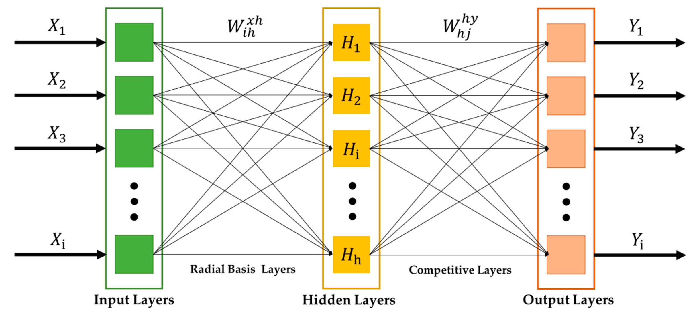
4. Probabilistic Neural Network for PQD Classification as a Classifier

To classify the type of power quality signals, the optimally selected features from the feature extraction obtained in Section 3 were passed through the classifier based on the PNN. Then, the dataset was trained and was used to classify the types of power quality signals, as shown in the flowchart of Figure 1. The PNN is one type of neural network that has been widely used as the classifier in PQD classification. It operates the neural network through the probabilistic model based on the Bayesian classifier for a pattern recognition system [46]. The main advantage of PNN is that its linear learning algorithms are capable of reaching similar results to the nonlinear learning algorithms, while conserving high accuracy. A simple implementation of PNN is also widely known for its distinctive merit, since the number of hidden layers and weights of the network are automatically defined by the network itself through the spread constant. In the literature, it has been widely shown that PNN is a highly capable tool for solving several types of classification problems [23,47,48,49]. Figure 3 shows that the PNN system comprises three layers: The input layer, hidden layer, and output layer. It is a radial network based on the Bayes strategy and the Parzen window. The initial weight value of each node is automatically initialized. The input data set are classified according to the distribution value or probability density function, $f_k(X)$, as given in Equation (7).

$$f_k(X)=\frac{1}{N_k}{\displaystyle \sum _{j=1}^{N_k}\exp \left(-\frac{\Vert X-X_{kj}\Vert }{2{\sigma }^2}\right)}$$

(7)

where $X$ represents the input vector, $\sigma$ is the standard deviation value, which is generally known as the spread constant or smoothing parameter, $N$ is the number of clusters, $j$ is the number of output layers, $k$ is the amount of training data, and the $\Vert X-X_{kj}\Vert$ term represents the Euclidean distance between $X$ and $X_{kj}$. The probability density function is utilized to obtain the output vector of the hidden layer of PNN, $H_h$, as written in Equation (8).

$$H_h=\exp \left(\frac{-{{\displaystyle {\sum }_i\left(X_i-W_{ih}^{xh}\right)}}^2}{2{\sigma }^2}\right)$$

(8)

where $W_{ih}^{xh}$ represents the connection weight between the input layers and the hidden layer, $i$ is the number of input layers and $h$ is the number of hidden layers. The network of PNN, net, can be calculated as Equation (9). Each pattern unit contributing to a signal has the same probability as its participated category unit. The test point is created by a Gaussian centered on the associated training point. The summation of these local estimations, computed at the corresponding category unit, provides the neural network as $ne{t}_j=\underset{k}{\max }\left(ne{t}_k\right)$, given in Equation (9).

$$\begin{gathered} ne{t}_j=\frac{1}{N_j}{\displaystyle \sum _h{W}_{hj}^{hy}{H}_h} \mathrm{and} N_j={\displaystyle \sum _h{W}_{hj}^{hy}} \\ ne{t}_j=\underset{k}{\max }\left(ne{t}_k\right) \mathrm{then} Y_j=1 \mathrm{else} Y_j=0 \end{gathered}$$

(9)

where $W_{hj}^{hy}$ is the connection weight between the output layers $Y$ and the hidden layers. The $\underset{k}{\max }\left(ne{t}_k\right)$ operation provides the desired category of the test point.

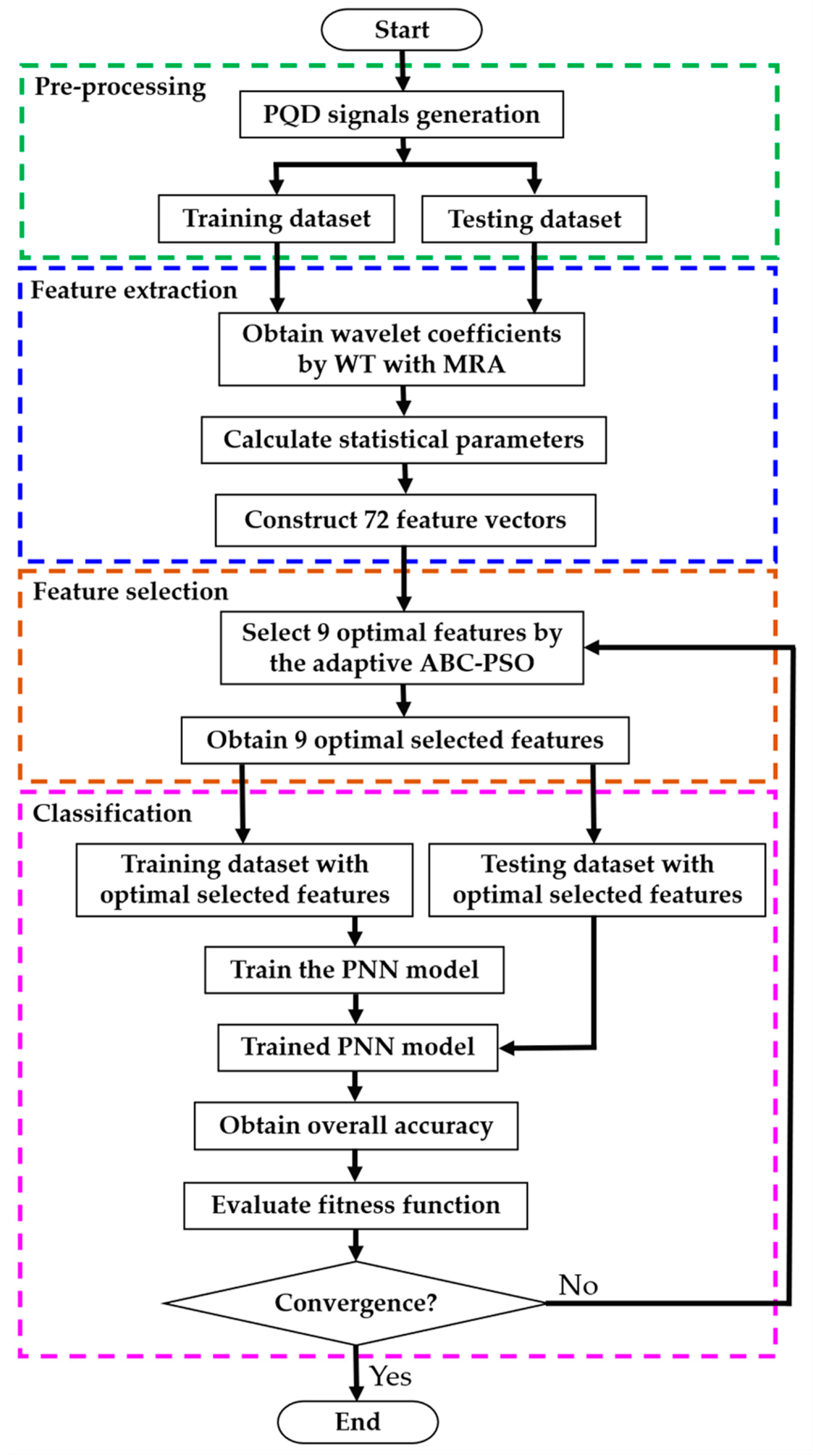
5. Proposed Adaptive ABC-PSO Algorithm as Optimal Feature Selection

The literature shows that the feature selection process is an important procedure in PQD classification, since this process can significantly impact the classification system’s performance indicators, i.e., the quantity of feature data obtained from feature extraction, processing time, and accuracy [38,39,40]. Figure 1 shows that the feature selection was performed to select the feature extracting data’s optimal features before it was passed through the classifier. We expected that the classification system could provide higher accuracy with a much shorter computational time based on the optimally selected data. We aimed to improve PQD classification performance by using a combination of adaptive ABC and PSO algorithms as a feature selection algorithm. This combination was motivated by the fact that the ABC algorithm can provide a high-quality solution, but its convergence rate is low; therefore, the fast convergence rate of the PSO algorithm might compensate for the drawbacks of the ABC algorithm. The proposed technique was also adapted to the ABC-PSO combination to improve the searchability of the ABC. Details of the proposed algorithm are described in the following sub-sections.

5.1. Artificial Bee Colony

The ABC is one of the swarm intelligent algorithms based on an emulation of honey bees seeking nectar [50,51]. This algorithm’s outstanding merits are a high-quality solution, good local search, and an updated solution mechanism. The type of bee grouping of the ABC algorithm is divided into three groups: The employed bee, onlooker bee, and scout bee. Each bee type typically finds the nectar source and exchanges the information with others until the best nectar source is found. The ABC algorithm procedure starts from the employed bee randomly searching the position of the best nectar and then memorizing the obtained position, as written in Equation (10). In this work, it is noted that the feature vector represents the position of the nectar.

$$v_{ij}=x_{ij}+{\phi }_{ij}\left(x_{ij}-x_{kj}\right)$$

(10)

where $x_{ij}$ is the feature vector, $v_{ij}$ is an updated vector according to the memorized feature vector, $i$ is the iteration number, $j$ is the feature dimension, $k$ is a random feature at each iteration, and $\phi$ is a random value between −1 and 1. The feature vector is updated by the onlooker bee, based on the result previously memorized by the employed bee. If the result obtained by the onlooker bee is higher than that of the observation bee, the existing result will be replaced by the updated feature data position. Then, all feature vectors collected by the employed bee are analyzed by the onlooker bee. The quality of the solution called fitness value, $fit\left({\theta }_i\right)$, is calculated from the fitness function, $f_i$, of the classifier, as given in Equation (11).

$$fi{t}_i=\frac{1}{1+f_i}$$

(11)

The probability of the highest solution related to the PQD classification accuracy, $p_i$, can be calculated using Equation (12).

$$p_i=\frac{fit\left({\theta }_i\right)}{{\displaystyle {\sum }_{i=1}^{S}fit\left({\theta }_i\right)}}$$

(12)

where ${\theta }_i$ is the accuracy of the feature vector and $S$ is the number of food souces, which is equal to the number of employed bees. Then, the probability of the fitness having the best solution is selected. An updated food position is calculated using Equation (13).

$$v_{ij}=z_{ij}+{\varphi }_{ij}\left(z_{ij}-z_{kj}\right)$$

(13)

where $v$ is an updated feature vector, $k$ is a random value, $\varphi$ is a random number between 0 and 1 in which the neighbor food sources are around $z$. The scout bee randomly searches the solution within their limited boundary, which is defined as “Limit”. If the iteration of the maximum cycle number and the fitness value of classification accuracy cannot be improved, it will be abandoned, and then the employed bee would turn into a scout bee. The expression for finding the new solution of the scout bee’s feature vector is given as Equation (14).

$$z_i^j=z_{\min }^j+rand\left(0,1\right)\left(z_{\max }^j-z_{\min }^j\right)$$

(14)

where $z_i^j$ is the abandoned feature vector, $j$ is the feature dimension, and $i$ is the iteration number.

5.2. Particle Swarm Optimization

The PSO algorithm is a kind of swarm intelligence technique that emulates a swarm’s foraging behavior, for example, birds, fish, ants, or bees [52]. The advantages of this algorithm are its simple implementation, good global optima, fast convergence, and short computational time [53]. The mechanism of the PSO algorithm is that the particles randomly move to find the best solution, and then the previous and the updated best positions throughout the maximum iteration number are recorded. The velocity of particles is updated using Equation (15), whereas the updated position of particles is expressed in Equation (16).

$$V_j^{i-1}=w{V}_j^i+c_1{r}_1(P_j^i-X_j^i)+c_2{r}_2(P_g^i-X_j^i)$$

(15)

$$X_j^{i-1}=X_j^i+V_j^{i+1}$$

(16)

where $j$ is the feature dimension, $V$ is the speed of feature dimension, $X$ is the position of feature dimension, $i$ is the iteration number, $w$ is the initial factor, $c_1$ and $c_2$ are the acceleration constants, $r_1$ and $r_2$ are random numbers between 0 to 1, $P$ is the best feature dimension position identified during its past iteration, and $P_g$ is the best global feature dimension position obtained from overall iterations.

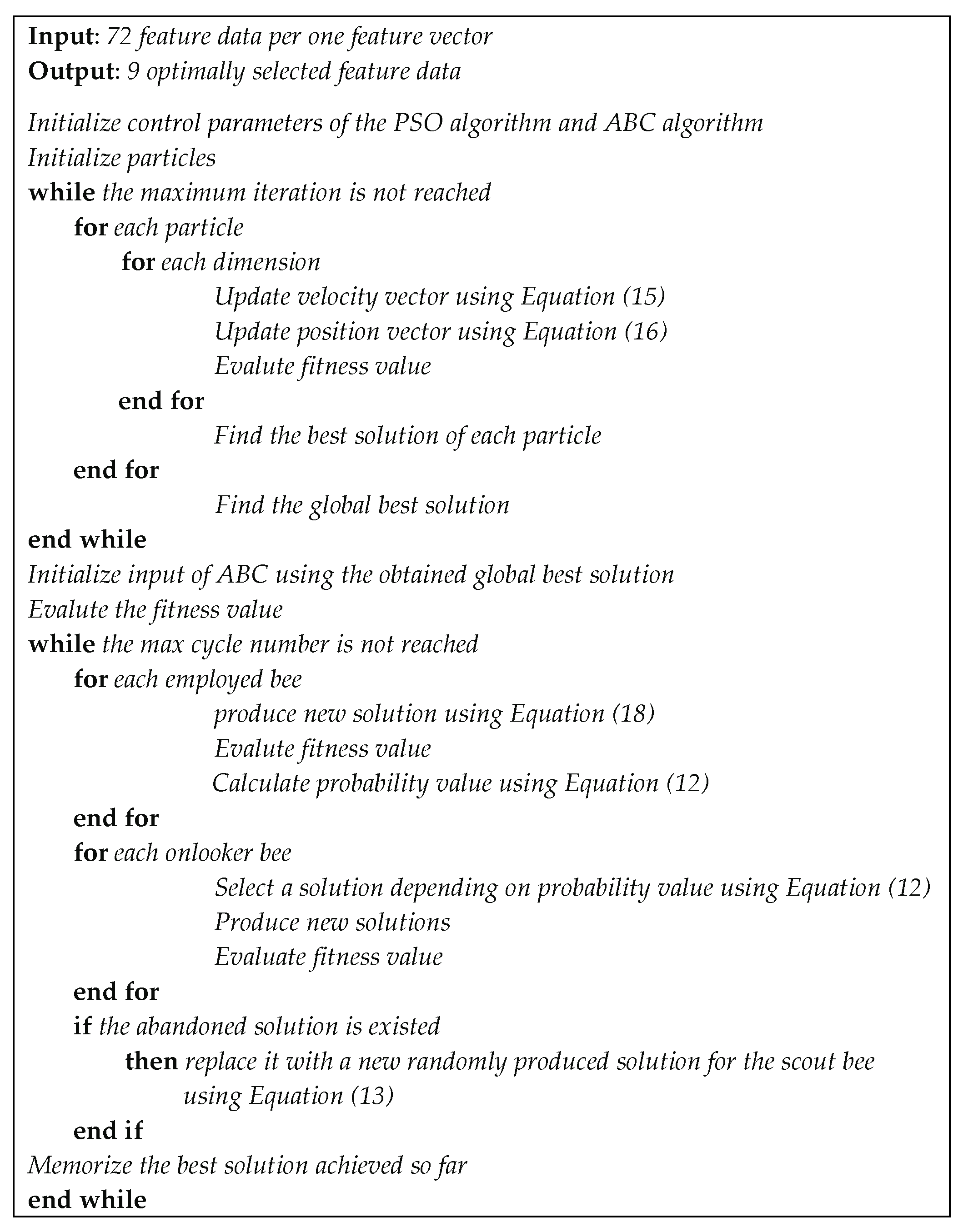
5.3. The Proposed Adaptive ABC-PSO Algorithm

As previously mentioned, we use the distinctive property of the PSO algorithm to compensate for the convergence weakness of the ABC algorithm (described in Section 5.1), aiming to improve the performance of PQD classification. An adaptive technique was also applied to the ABC algorithm to improve the searching resolution of the overall algorithm. The procedure to implement the adaptive ABC-PSO algorithm as the feature selection algorithm of PQD classification is shown in the pseudocode of Figure 4 and is detailed as follows.

Step 1: Initialize the control parameters of PSO and ABC algorithms, including the initial speed, position, and number of particles of the PSO algorithm.

Step 2: Determine the solution of the PSO algorithm. All feature vectors are compared in order to select the one having the best solution (highest classification accuracy). After that, calculate the fitness value of the selected optimal feature vector. In this work, the accuracy of identifying each type of PQD is defined as a ratio of the numbers of correctly classified signal types to the numbers of test signals. The overall accuracy (classification accuracy) is defined as the average accuracy of all signal types.

Step 3: The highest classification accuracy obtained from the PSO algorithm is adopted as the initial solution of the ABC algorithm. Then, obtain a new vector feature by using the adaptive ABC, as in the following details. In this work, we enhanced the exploration of the ABC-PSO algorithm by enlarging the employed bee’s search space, while finding the new position of best nectar. This process aims to achieve a better solution that could be located near the previously obtained solution; therefore, the improved random value of the proposed self-adaptive bee colony technique is redefined based on the random value of the previous iteration, as given in Equation (17).

$${\phi }_{ij}^k={\phi }_{ij}^{k-1}-\frac{C\left(w_{\max }-w_{\min }\right)}{C_{\max }}$$

(17)

where ${\phi }_{ij}^k$ is a random value obtained from the previous iteration. $w_{\max }$ and $w_{\min }$ are the initial and the final weights, respectively, $C$ is the current iteration of the adaptive process, $C_{\max }$ is the number of iterations of the adaptive process, $j$ is the feature dimension, $i$ is the iteration number of the employed bee phase, and $k$ is the iteration of the updated random value. Then, one randomly selected element of the feature vector is replaced by the improved random value to generate the updated vector feature, as written in Equation (18).

$$v_{ij}=x_{ij}+{\phi }_{ij}^k\left(x_{ij}-x_{kj}\right)$$

(18)

Next, calculate the fitness value of the classification accuracy of each feature vector. If the result obtained by the adaptive ABC algorithm is better than that of the PSO algorithm, the PSO algorithm’s optimal feature is replaced by that of the adaptive ABC algorithm.

Step 4: The onlooker bee selects a feature vector according to the quantity of the optimal feature following the probability function, shown in Equation (12).

Step 5: The scout bee randomly generates the feature vector of the next iteration using Equation (13) and then evaluates the optimal feature.

Step 6: The optimal feature vector is selected, while the fitness value is collected and used as the input data of the feature selection.

6. Results and Discussion

The PQD classification system’s performance based on the proposed adaptive ABC-PSO as a feature selection algorithm was evaluated under the 13 power quality signal types. The feature extraction of the presented classification system was based on the DWT, while the PNN was performed as the classifier. The simulations were based on a MATLAB program. The mechanism of the adaptive ABC-PSO as optimal feature selection algorithm is described in detail in Section 6.1. The classification performance is then demonstrated in Section 6.2; classification under a noisy environment is shown in Section 6.3. A convergence rate profile is presented in Section 6.4. The classification performance based on the real data of the distribution network is discussed in Section 6.5. Lastly, a performance comparison between the presented classification system and the other existing methods is indicated in Section 6.6.

6.1. Mechanism of the Proposed Adaptive ABC-PSO Algorithm as Optimal Feature Selection

Table 4. The feature vector and the selected features by the adaptive ABC-PSO algorithm.

Wavelet Coefficients	Statistical Parameters
	Energy	Entropy	S.D.	Mean	Kurtosis	Skewness	RMS	Range
$D_1$	1	2	3	4	5	6	7	8
$D_2$	9	10	11	12	13	14	15	16
$D_3$	17	18	19	20	21	22	23	24
$D_4$	25	26	27	28	29	30	31	32
$D_5$	33	34	35	36	37	38	39	40
$D_6$	41	42	43	44	45	46	47	48
$D_7$	49	50	51	52	53	54	55	56
$D_8$	57	58	59	60	61	62	63	64
$A_8$	65	66	67	68	69	70	71	72

shows all 72 features obtained from the DWT feature extraction through the MRA coefficients. The best statistical parameters of each wavelet coefficient that could provide the highest classification accuracy were selected by the adaptive ABC-PSO algorithm, as shown by the squares in Table 4. The quantity of optimal selected features corresponded to the number of signal coefficients obtained from feature extraction. Further details of the classification accuracy as a function of iteration number, spread constant, and selected features are reported in

Table 5. The classification accuracy and the selected features by the adaptive ABC-PSO algorithm as a function of iteration number and spread constant.

Iteration	Optimal Features									Spread Constant	Overall Accuracy (%)
724	8	16	18	28	40	47	54	63	69	0.0009286	98.92
725	2	14	23	31	38	41	50	63	65	0.0009286	95.23
726	3	16	17	31	36	44	49	60	67	0.0005143	98.62
727	5	9	21	25	35	45	50	60	72	0.0003071	96.31
728	5	16	18	32	40	41	52	58	68	0.0018460	99.31
729	7	16	17	30	37	41	53	58	71	0.0015500	96.38
730	3	11	18	27	40	41	52	60	68	0.0003071	98.92
731	6	16	18	26	40	48	49	58	66	0.0009286	98.92
732	5	16	17	29	37	41	54	64	67	0.0015500	98.00

. It was found that the highest classification accuracy of 99.31% was achieved at iteration 728. The nine selected optimal statistical parameters were 5, 16, 18, 32, 40, 41,52, 58, and 68; the related spread constant is indicated.

6.2. Accuracy of the PQD Classification Using the Adaptive ABC-PSO Algorithm as Optimal Feature Selection

The accuracy of the PQD classification both with and without using the proposed adaptive ABC-PSO algorithm as optimal feature selection, based on 100 tests, is shown in

Table 6. Classification accuracy.

Type of PQD	Accuracy (%)
	One Type (Energy)	One Type (Entropy)	One Type (S.D.)	Three Types (Energy + Entropy + S.D.)	Five Types (Energy + Entropy + S.D. + Mean + Kurtosis)	All Types	Optimal Adaptive ABC-PSO
Pure sine	100	100	100	100	100	100	100
Sag	93	77	80	96	96	97	98
Swell	93	69	76	94	98	99	98
Interruption	100	94	87	100	100	100	100
Harmonic	100	79	100	99	100	100	100
Sag with harmonic	92	71	81	95	94	89	98
Swell with harmonic	89	72	75	91	95	98	100
Interruption with harmonic	98	92	93	99	98	100	99
Flicker	98	92	96	98	99	99	99
Oscillatory transient	97	95	81	96	96	99	99
Impulsive transient	99	95	98	100	100	100	100
Periodic notch	100	100	100	100	100	100	100
Spike	100	100	100	100	100	100	100
Overall	96.84	87.38	89.77	97.54	98.15	98.54	99.31

. Table 6 shows that the classification accuracy based on a single statistical parameter is about 87.38–96.84%, which falls in the low-range scale of classification compared to the other existing techniques. Thus, multiple statistical parameters are typically required in the PQD classification to improve classification accuracy. Results also show that using three and five statistical parameters could provide an overall accuracy of 97.54% and 98.15%, respectively. Meanwhile, a classification accuracy of 98.54% was obtained by using all statistical parameters. By comparing the overall accuracy achieved by the PNN classifier excluding feature selection with the existed literature, we found that our classification accuracy of 98.54% are higher than that shown in Reference [11] (96.11%), Reference [36] (94.4%), Reference [40] (94.4%), Reference [49] (98.42%), Reference [51] (97.6%), Reference [52] (98%), and Reference [53] (98.08%). It was found that an overall accuracy of up to 99.31% was achieved when nine optimally selected features were used in the feature selection process. In this case, it is also unnecessary to use all features in the classification process, which significantly reduces computational time; therefore, the proposed adaptive ABC-PSO as optimal feature selection algorithm indicates high performance in PQD classification.

6.3. Classification Accuracy under a Noisy Environment

Since a noisy situation is typical in a practical electrical distribution system, the presented PQD classification system’s performance under a noisy environment was also tested. The white noise added signals with a signal-to-noise ratio of 10, 20, 30, 40, and 50 dB were uniformly applied to the power quality signals.

Table 7. Classification accuracy under a noisy environment.

Magnitude of Noise	Classification Accuracy (%)
	All Features	Optimal Selected Features by PSO	Optimal Selected Features by ABC	Optimal Selected Features by ABC-PSO
10 dB	77.54	73.97	76.00	79.62
20 dB	89.66	88.00	88.68	88.68
30 dB	95.57	95.14	95.38	95.45
40 dB	96.92	96.12	96.31	97.23
50 dB	98.28	97.91	98.28	98.40

shows that the classification system using the optimal feature selection algorithm indicates a higher durability to the noise than that without using optimal feature selection and using ABC and PSO; therefore, the proposed PQD classification system could operate well in a noisy environment.

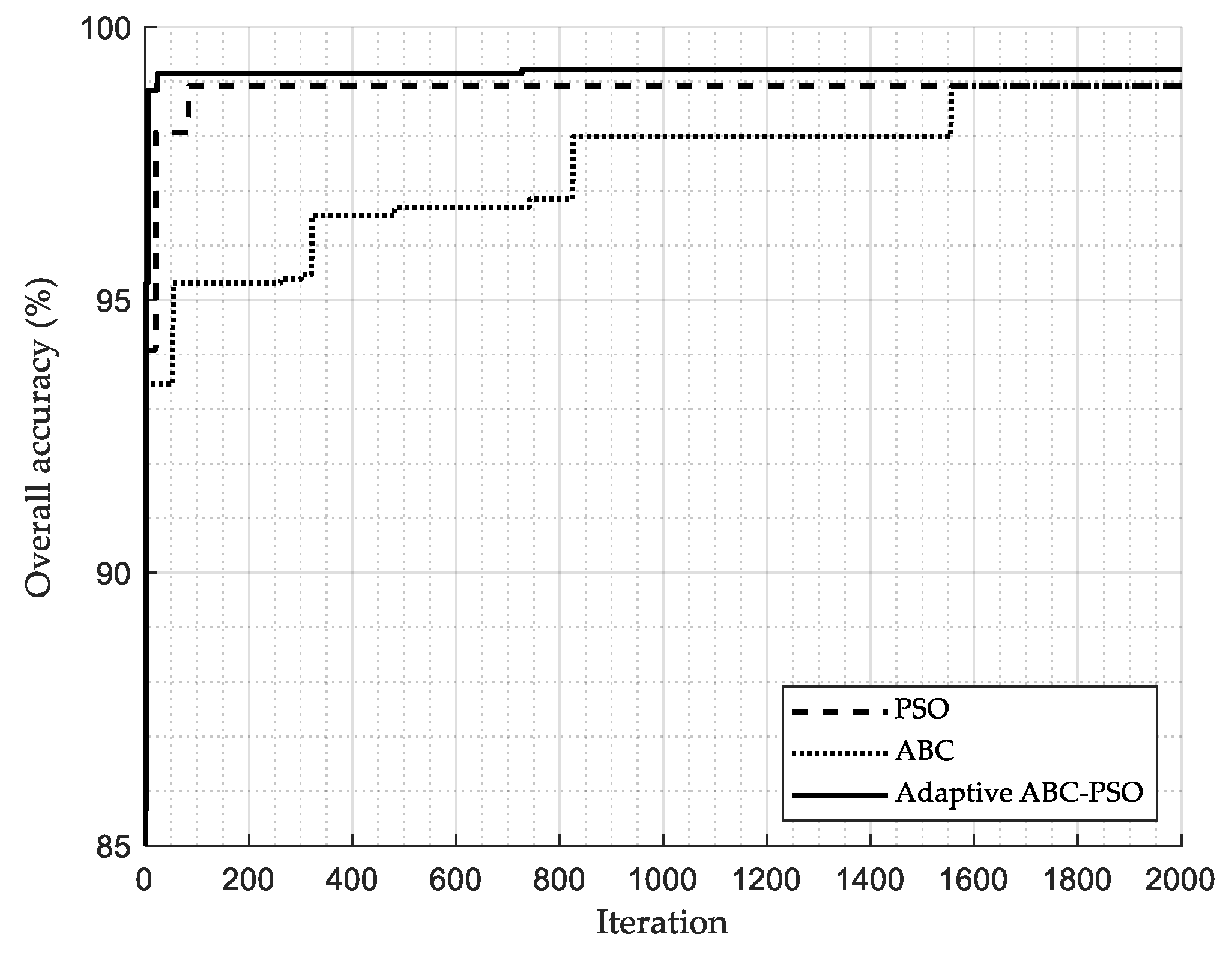
6.4. Convergence Rate

As mentioned above, we aimed to adapt the fast convergence rate property of the PSO to compensate for the low convergence rate of the ABC. Figure 5 compares the convergence rate of the PSO, ABC, and adaptive ABC-PSO algorithms. In this work, the convergence rate is determined based on the iteration in which the best solution is reached. It is noted that the number of iterations must be sufficient to cover the steady-state of solutions. As expected, the PSO algorithm has the highest convergence rate to reach the best solution (iteration 84); meanwhile, the ABC algorithm has a worse convergence rate than others (iteration 1556), as shown in

Table 8. Comparison of the convergence rate of nine optimal selected features.

Feature Selection Algorithm	Number of Iterations Required
PSO	84
ABC	1556
ABC-PSO	728

. Remarkably, the results indicate that the adaptive ABC-PSO can reach the highest overall accuracy at iteration 728, showing that the strength of PSO can greatly enhance the weakness of the ABC. Nevertheless, the adaptive ABC-PSO convergence rate is still lower than the PSO algorithm because it contains the ABC algorithm. Although we attempted to improve the convergence rate of the proposed algorithm, it must be kept in mind that an overall accuracy has the highest priority in PQD classification; therefore, it is clear that the ABC-PSO algorithm indicates the highest performance in this case. Hence, the feature selection based on the adaptive ABC-PSO algorithm not only provides high classification accuracy, but the best solution can also be found within a shorter time.

6.5. Classification Performance Based on the Real Data of a Distribution Network

Table 9. Classification accuracy based on a real dataset of a distribution network.

Type of PQDs	Test Number	Classification Accuracy by the Proposed Adaptive ABC-PSO
Pure sine	100	99
Sag	100	98
Swell	100	100
Interruption	100	99
Harmonic	100	100
Overall		99.2

shows the classification accuracy based on the real dataset of a distribution network in China, Singapore, South Africa, and Sweden. The dataset was adopted from PQube equipment, an instrument for power quality monitoring and real-time electrical signal phenomena recoding [54]. The classification accuracy was based on the optimally selected features. The classification system based on the proposed adaptive ABC-PSO algorithm as feature selection demonstrates the classification accuracy of 99.2%, which is consistent with the accuracy, shown in Table 6; therefore, the proposed algorithm not only provides high accuracy to classify the standard waveforms of PQD, but it can also accurately classify the PDQs in a real distribution system.

6.6. Performance Comparison to the Existing PQD Classification Systems

The PQD classification performance using the adaptive ABC-PSO algorithm as optimal feature selection was compared to the other existing methods, as shown in

Table 10. A comparison of classification accuracy with previous studies.

Reference	Number of PQD Types	Feature Extraction Type	Classification Technique	Optimal Feature Selection Algorithm	Overall Accuracy (%)
[40]	5	DWT	least squares SVM	k-means+Apriori algorithm	98.88
[55]	9	ST	Fuzzy C-means	Adaptive PSO	96.33
[14]	9	ST+VMD	support vector machine (SVM)	SFS	99.66
[41]	10	DWT	extreme learning machine (ELM)	PSO	97.60
[56]	13	VMD	one-versus-rest SVM	Permutation Entropy+Fisher Score	97.6
[57]	13	hyperbolic S-transform	Decision tree	GA	99.5
[58]	15	VMD	polynomial fast reduced kernel ELM	FDA	98.82
This work	13	WT	PNN	Adaptive ABC-PSO	99.31

. The overall accuracy of each method was adopted from the mentioned references. The adaptive ABC-PSO algorithm could provide high classification accuracy of 99.31% for identifying 13 types of power quality signals. The classification accuracy achieved by the proposed method is higher than most of the existing methods and is classified as a very-high precision range. Although our proposed algorithm has a slightly lower accuracy than that shown in Reference [52] under the same PQD signal types, the proposed algorithm’s convergence rate could be much better, due to the use of their GA selection algorithm; therefore, the proposed optimal feature selection algorithm is suitable for practical PQD classification.

7. Conclusions

In this article, a high-accuracy PQD classification, based on the adaptive ABC-PSO algorithm as optimal feature selection, was introduced to classify the 13 types of power quality signals. The feature extraction was based on the DWT, while the PNN performed as the classifier. The nine optimal features were selected by the optimal feature selection algorithm. The results show that the optimal features’ classification accuracy was higher than that based on other numerical features. The highest classification accuracy of 99.31% could be achieved by using the optimally selected features. The proposed PQD classification system also indicated a high performance under a noisy environment. In addition, the classification accuracy, based on the real dataset of a distribution network, was consistent with that based on the standard waveforms. When comparing the performance of the presented PQD classification system to previous studies, the PQD classification accuracy using the adaptive ABC-PSO as optimal feature selection algorithm is classified as the high precision range; therefore, the adaptive ABC algorithm is suitable for implementation of PQD classification in electrical distribution systems.

References

1. Muangthai, I.; Lin, S.J.; Lewis, C. Inter-industry linkages, energy and CO2 multipliers of the electric power industry in thailand. Aerosol Air Qual. Res. 2016, 16, 2033–2047. [Google Scholar] [CrossRef]
2. Khaboot, N.; Srithapon, C.; Siritaratiwat, A.; Khunkitti, P. Increasing benefits in high PV penetration distribution system by using battery enegy storage and capacitor placement based on Salp Swarm algorithm. Energies 2019, 12, 4817. [Google Scholar] [CrossRef] [Green Version]
3. Khaboot, N.; Chatthaworn, R.; Siritaratiwat, A.; Surawanitkun, C.; Khunkitti, P.; Meng, W. Increasing PV penetration level in low voltage distribution system using optimal installation and operation of battery energy storage. Cogent Eng. 2019, 6, 1641911. [Google Scholar] [CrossRef]
4. Karasu, S.; Saraç, Z. Classification of power quality disturbances by 2D-Riesz Transform, multi-objective grey wolf optimizer and machine learning methods. Digit. Signal Process. 2020, 101, 102711. [Google Scholar] [CrossRef]
5. Cai, K.; Hu, T.; Cao, W.; Li, G. Classifying power quality disturbances based on phase space reconstruction and a convolutional neural network. Appl. Sci. 2019, 9, 3681. [Google Scholar] [CrossRef] [Green Version]
6. Onlam, A.; Yodphet, D.; Chatthaworn, R.; Surawanitkun, C.; Siritaratiwat, A.; Khunkitti, P. Power loss minimization and voltage stability improvement in electrical distribution system via network reconfiguration and distributed generation placement using novel adaptive shuffled frogs leaping algorithm. Energies 2019, 12, 553. [Google Scholar] [CrossRef] [Green Version]
7. IEEE. IEEE 1159-2019—IEEE Recommended Practice for Monitoring Electric Power Quality; IEEE: New York, NY, USA, 2019. [Google Scholar]
8. CENELEC—EN 50160—Voltage Characteristics of Electricity Supplied by Public Electricity Networks. Available online: https://standards.globalspec.com/std/13493775/EN50160 (accessed on 3 December 2020).
9. IEC 61000-4-30:2015 RLV—IEC Webstore—Electromagnetic Compatibility, EMC, Smart City. Available online: https://webstore.iec.ch/publication/22270 (accessed on 3 December 2020).
10. Mishra, M. Power quality disturbance detection and classification using signal processing and soft computing techniques: A comprehensive review. Int. Trans. Electr. Energy Syst. 2019, 29, e12008. [Google Scholar] [CrossRef] [Green Version]
11. Wang, J.; Xu, Z.; Che, Y. Power quality disturbance classification based on dwt and multilayer perceptron extreme learning machine. Appl. Sci. 2019, 9, 2315. [Google Scholar] [CrossRef] [Green Version]
12. Khokhar, S.; Zin, A.A.B.M.; Mokhtar, A.S.B.; Pesaran, M. A comprehensive overview on signal processing and artificial intelligence techniques applications in classification of power quality disturbances. Renew. Sustain. Energy Rev. 2015, 51, 1650–1663. [Google Scholar] [CrossRef]
13. Singh, U.; Singh, S.N. Application of fractional Fourier transform for classification of power quality disturbances. IET Sci. Meas. Technol. 2017, 11, 67–76. [Google Scholar] [CrossRef]
14. Abdoos, A.A.; Mianaei, P.K.; Ghadikolaei, M.R. Combined VMD-SVM based feature selection method for classification of power quality events. Appl. Soft Comput. 2016, 38, 637–646. [Google Scholar] [CrossRef]
15. Zhong, T.; Zhang, S.; Cai, G.; Li, Y.; Yang, B.; Chen, Y. Power quality disturbance recognition based on multiresolution S-transform and decision tree. IEEE Access 2019, 7, 88380–88392. [Google Scholar] [CrossRef]
16. Thirumala, K.; Prasad, M.S.; Jain, T.; Umarikar, A.C. Tunable-Q wavelet transform and dual multiclass SVM for online automatic detection of power quality disturbances. IEEE Trans. Smart Grid 2018, 9, 3018–3028. [Google Scholar] [CrossRef]
17. Karasu, S.; Saraç, Z. Investigation of power quality disturbances by using 2D discrete orthonormal S-transform, machine learning and multi-objective evolutionary algorithms. Swarm Evol. Comput. 2019, 44, 1060–1072. [Google Scholar] [CrossRef]
18. Erişti, H.; Demir, Y. A new algorithm for automatic classification of power quality events based on wavelet transform and SVM. Expert Syst. Appl. 2010, 37, 4094–4102. [Google Scholar] [CrossRef]
19. Li, J.; Teng, Z.; Tang, Q.; Song, J. Detection and classification of power quality disturbances using double resolution S-transform and DAG-SVMs. IEEE Trans. Instrum. Meas. 2016, 65, 2302–2312. [Google Scholar] [CrossRef]
20. Biswal, B.; Dash, P.; Panigrahi, B. Non-stationary power signal processing for pattern recognition using HS-transform. Appl. Soft Comput. 2009, 9, 107–117. [Google Scholar] [CrossRef]
21. Singh, H.R.; Mohanty, S.R.; Kishor, N.N.; Thakur, K.A. Real-time implementation of signal processing techniques for disturbances detection. IEEE Trans. Ind. Electron. 2018, 66, 3550–3560. [Google Scholar] [CrossRef]
22. Santos, G.G.; Menezes, T.S.; Vieira, J.C.M.; Barra, P.H.A. An S-transform based approach for fault detection and classification in power distribution systems. In Proceedings of the 2019 IEEE Power & Energy Society General Meeting (PESGM), Atlanta, GA, USA, 4–8 August 2019; pp. 1–5. [Google Scholar] [CrossRef]
23. Aker, E.; Othman, M.L.; Veerasamy, V.; Bin Aris, I.; Wahab, N.I.A.; Hizam, H. Fault detection and classification of shunt compensated transmission line using discrete wavelet transform and naive Bayes classifier. Energies 2020, 13, 243. [Google Scholar] [CrossRef] [Green Version]
24. Montoya, F.G.; Baños, R.; Alcayde, A.; Montoya, M.G.; Manzano-Agugliaro, F. Power quality: Scientific collaboration networks and research trends. Energies 2018, 11, 2067. [Google Scholar] [CrossRef] [Green Version]
25. Ferreira, V.; Zanghi, R.; Fortes, M.; Sotelo, G.; Silva, R.; Souza, J.; Guimarães, C.; Gomes, S. A survey on intelligent system application to fault diagnosis in electric power system transmission lines. Electr. Power Syst. Res. 2016, 136, 135–153. [Google Scholar] [CrossRef]
26. Mandal, P.; Madhira, S.T.S.; Ul haque, A.; Meng, J.; Pineda, R.L. Forecasting power output of solar photovoltaic system using wavelet transform and artificial intelligence techniques. Procedia Comput. Sci. 2012, 12, 332–337. [Google Scholar] [CrossRef] [Green Version]
27. Saini, M.K.; Kapoor, R. Classification of power quality events—A review. Int. J. Electr. Power Energy Syst. 2012, 43, 11–19. [Google Scholar] [CrossRef]
28. Gunal, S.; Gerek, O.N.; Ece, D.G.; Edizkan, R. The search for optimal feature set in power quality event classification. Expert Syst. Appl. 2009, 36, 10266–10273. [Google Scholar] [CrossRef]
29. Ekici, S.; Yildirim, S.; Poyraz, M. Energy and entropy-based feature extraction for locating fault on transmission lines by using neural network and wavelet packet decomposition. Expert Syst. Appl. 2008, 34, 2937–2944. [Google Scholar] [CrossRef]
30. Hooshmand, R.; Enshaee, A. Detection and classification of single and combined power quality disturbances using fuzzy systems oriented by particle swarm optimization algorithm. Electr. Power Syst. Res. 2010, 80, 1552–1561. [Google Scholar] [CrossRef]
31. Bizjak, B.; Planinšič, P. Classification of power disturbances using fuzzy logic. In Proceedings of the 2006 12th International Power Electronics and Motion Control Conference, Portoroz, Slovenia, 30 August–1 September 2006; pp. 1356–1360. [Google Scholar]
32. Wang, M.-H.; Tseng, Y.-F. A novel analytic method of power quality using extension genetic algorithm and wavelet transform. Expert Syst. Appl. 2011, 38, 12491–12496. [Google Scholar] [CrossRef]
33. Bravo-Rodríguez, J.C.; Torres, F.J.; Borrás, M.D. Hybrid machine learning models for classifying power quality disturbances: A comparative study. Energies 2020, 13, 2761. [Google Scholar] [CrossRef]
34. Huang, N.; Zhang, S.; Cai, G.; Xu, D. Power quality disturbances recognition based on a multiresolution generalized S-transform and a PSO-improved decision tree. Energies 2015, 8, 549–572. [Google Scholar] [CrossRef]
35. Mishra, S.; Bhende, C.N.; Panigrahi, B.K. Detection and classification of power quality disturbances using S-transform and probabilistic neural network. IEEE Trans. Power Deliv. 2007, 23, 280–287. [Google Scholar] [CrossRef]
36. Monedero, I.; Leon, C.; Ropero, J.; Garcia, A.; Elena, J.M.; Montano, J.C. Classification of electrical disturbances in real time using neural networks. IEEE Trans. Power Deliv. 2007, 22, 1288–1296. [Google Scholar] [CrossRef]
37. Bhende, C.; Mishra, S.; Panigrahi, B. Detection and classification of power quality disturbances using S-transform and modular neural network. Electr. Power Syst. Res. 2008, 78, 122–128. [Google Scholar] [CrossRef]
38. Singh, U.; Singh, S.N. Optimal feature selection via NSGA-II for power quality disturbances classification. IEEE Trans. Ind. Inform. 2018, 14, 2994–3002. [Google Scholar] [CrossRef]
39. Huang, N.; Peng, H.; Cai, G.; Chen, J. Power quality disturbances feature selection and recognition using optimal multi-resolution fast S-transform and CART algorithm. Energies 2016, 9, 927. [Google Scholar] [CrossRef] [Green Version]
40. Erişti, H.; Yıldırım, Ö.; Erişti, B.; Demir, Y. Optimal feature selection for classification of the power quality events using wavelet transform and least squares support vector machines. Int. J. Electr. Power Energy Syst. 2013, 49, 95–103. [Google Scholar] [CrossRef]
41. Ahila, R.; Sadasivam, V.; Manimala, K. An integrated PSO for parameter determination and feature selection of ELM and its application in classification of power system disturbances. Appl. Soft Comput. 2015, 32, 23–37. [Google Scholar] [CrossRef]
42. Ucar, F.; Alcin, O.F.; Dandil, B.; Ata, F. Power quality event detection using a fast extreme learning machine. Energies 2018, 11, 145. [Google Scholar] [CrossRef] [Green Version]
43. Hajian, M.; Foroud, A.A. A new hybrid pattern recognition scheme for automatic discrimination of power quality disturbances. Measurement 2014, 51, 265–280. [Google Scholar] [CrossRef]
44. Radil, T.; Ramos, P.M.; Janeiro, F.M.; Serra, A.C. PQ monitoring system for real-time detection and classification of disturbances in a single-phase power system. IEEE Trans. Instrum. Meas. 2008, 57, 1725–1733. [Google Scholar] [CrossRef]
45. Ray, P.K.; Kishor, N.; Mohanty, S.R. Islanding and power quality disturbance detection in grid-connected hybrid power system using wavelet and S-transform. IEEE Trans. Smart Grid 2012, 3, 1082–1094. [Google Scholar] [CrossRef]
46. Huang, N.; Xu, D.; Liu, X.; Lin, L. Power quality disturbances classification based on S-transform and probabilistic neural network. Neurocomputing 2012, 98, 12–23. [Google Scholar] [CrossRef]
47. Mohanty, S.R.; Ray, P.K.; Kishor, N.; Panigrahi, B. Classification of disturbances in hybrid DG system using modular PNN and SVM. Int. J. Electr. Power Energy Syst. 2013, 44, 764–777. [Google Scholar] [CrossRef]
48. Sharma, R.; Pachori, R.B.; Acharya, U.R. An integrated index for the identification of focal electroencephalogram signals using discrete wavelet transform and entropy measures. Entropy 2015, 17, 5218–5240. [Google Scholar] [CrossRef] [Green Version]
49. Beritelli, F.; Capizzi, G.; Sciuto, G.L.; Napoli, C.; Scaglione, F. Rainfall estimation based on the intensity of the received signal in a LTE/4G Mobile terminal by using a probabilistic neural network. IEEE Access 2018, 6, 30865–30873. [Google Scholar] [CrossRef]
50. Karaboga, D. An Idea Based on Honey Bee Swarm for Numerical Optimization; Technical Report-TR06; Erciyes University: Talas, Turkey, 2005. [Google Scholar]
51. Karaboga, D.; Basturk, B. A powerful and efficient algorithm for numerical function optimization: Artificial bee colony (ABC) algorithm. J. Glob. Optim. 2007, 39, 459–471. [Google Scholar] [CrossRef]
52. Karaboga, D.; Akay, B. A survey: Algorithms simulating bee swarm intelligence. Artif. Intell. Rev. 2009, 31, 61–85. [Google Scholar] [CrossRef]
53. Chen, J.-F.; Do, Q.H.; Hsieh, H.-N. Training artificial neural networks by a hybrid PSO-CS algorithm. Algorithms 2015, 8, 292–308. [Google Scholar] [CrossRef]
54. Available online: http://map.pqube.com/ (accessed on 10 February 2021).
55. Biswal, B.; Dash, P.K.; Panigrahi, B.K. Power quality disturbance classification using fuzzy C-means algorithm and adaptive particle swarm optimization. IEEE Trans. Ind. Electron. 2009, 56, 212–220. [Google Scholar] [CrossRef]
56. Fu, L.; Zhu, T.; Pan, G.; Chen, S.; Zhong, Q.; Wei, Y. Power quality disturbance recognition using VMD-based feature extraction and heuristic feature selection. Appl. Sci. 2019, 9, 4901. [Google Scholar] [CrossRef] [Green Version]
57. Ray, P.K.; Mohanty, S.R.; Kishor, N.; Catalao, J.P.S. Optimal feature and decision tree-based classification of power quality disturbances in distributed generation systems. IEEE Trans. Sustain. Energy 2014, 5, 200–208. [Google Scholar] [CrossRef]
58. Chakravorti, T.; Dash, P.K. Multiclass power quality events classification using variational mode decomposition with fast reduced kernel extreme learning machine-based feature selection. IET Sci. Meas. Technol. 2018, 12, 106–117. [Google Scholar] [CrossRef]
Figure 1. The flowchart of PQD classification. PNN, probabilistic neural network; ABC, artificial bee colony; PSO, particle swarm optimization; WT, wavelet transform; MRA, multi-resolution analysis.
Energies 14 01238 g001
Figure 2. The process of MRA.
Energies 14 01238 g002
Figure 3. The architecture of PNN.
Energies 14 01238 g003
Figure 4. Pseudocode of the proposed adaptive ABC-PSO algorithm.
Energies 14 01238 g004
Figure 5. Comparison of the convergence rate of different feature selection algorithms.
Energies 14 01238 g005