Testing Stability of Digital Filters Using Optimization Methods with Phase Analysis

Abstract

In this paper, novel methods for the evaluation of digital-filter stability are investigated. The methods are based on phase analysis of a complex function in the characteristic equation of a digital filter. It allows for evaluating stability when a characteristic equation is not based on a polynomial. The operation of these methods relies on sampling the unit circle on the complex plane and extracting the phase quadrant of a function value for each sample. By calculating function-phase quadrants, regions in the immediate vicinity of unstable roots (i.e., zeros), called candidate regions, are determined. In these regions, both real and imaginary parts of complex-function values change signs. Then, the candidate regions are explored. When the sizes of the candidate regions are reduced below an assumed accuracy, then filter instability is verified with the use of discrete Cauchy’s argument principle. Three different algorithms of the unit-circle sampling are benchmarked, i.e., global complex roots and poles finding (GRPF) algorithm, multimodal genetic algorithm with phase analysis (MGA-WPA), and multimodal particle swarm optimization with phase analysis (MPSO-WPA). The algorithms are compared in four benchmarks for integer- and fractional-order digital filters and systems. Each algorithm demonstrates slightly different properties. GRPF is very fast and efficient; however, it requires an initial number of nodes large enough to detect all the roots. MPSO-WPA prevents missing roots due to the usage of stochastic space exploration by subsequent swarms. MGA-WPA converges very effectively by generating a small number of individuals and by limiting the final population size. The conducted research leads to the conclusion that stochastic methods such as MGA-WPA and MPSO-WPA are more likely to detect system instability, especially when they are run multiple times. If the computing time is not vitally important for a user, MPSO-WPA is the right choice, because it significantly prevents missing roots.

1. Introduction

Stability analysis is an important topic in almost every area of engineering. Most electronic circuits must be stable to operate properly and to execute tasks for which they are designed. It is also vitally important in digital signal processing. In general, the discrete-time linear time-invariant (LTI) system is (asymptotically) stable if and only if all the roots (i.e., zeros) of the characteristic equation ($f\left(z\right)=0$) are within the unit circle on the complex z-plane [1,2,3]. A direct approach to testing stability is to find all the zeros of the characteristic equation (e.g., a denominator of a transfer function). However, this might be a difficult task because, for some systems, e.g., those of fractional order [4,5], the characteristic equation may not be based on a polynomial. To prove the system stability, one has to show that there are no roots of the characteristic equation in an infinite region outside the unit circle ($\left|z\right|>1$). However, despite the progress in computational techniques, root finding for complex functions of complex variables remains an open scientific problem [6,7,8,9,10,11,12,13,14,15].

For fractional-order systems, one can employ the graphical method proposed in [16] to evaluate the system stability. By means of one-to-one transformation, the region of stability on the complex plane is obtained, for which the parameter values inside it guarantee the stability of the system. In [4,5], the stability criterion for fractional-order systems is used to offer simple numerical procedures for testing the system stability. In [17], a modification of the Mikhailov stability criterion is formulated, which can be used to test the stability of discrete-time fractional-order systems. However, none of the aforementioned methods is general enough to be used to test the stability of discrete-time systems with arbitrary characteristic equations (e.g., those being interconnections of various fractional-order systems [18]). Therefore, we investigate general numerical techniques that allow for testing the stability of arbitrary systems based solely on the characteristic equation, hence without any significant analytical preprocessing.

We already proposed numerical tests [19,20] for evaluation of the system stability by employing modern techniques of global root finding based on Delaunay’s triangulation [21,22]. In [18], the global complex roots and poles finding (GRPF) algorithm was implemented to test the stability of discrete-time LTI systems. Furthermore, we recently developed two novel roots and poles finding methods that combine efficient evolutionary algorithms, called multimodal genetic algorithm with phase analysis (MGA-WPA) [23] and multimodal particle swarm optimization with phase analysis (MPSO-WPA) [24,25]. Each of these methods employ complex-function phase analysis and discrete Cauchy’s argument principle (DCAP); hence, they are not sensitive to numerical precision issues resulting from overflow of arithmetic operations. The motivation behind this work is to benchmark and compare the abovementioned methods in stability tests targeting discrete-time LTI systems, especially digital filters.

This work is an extension of a conference paper [24]. This extension covers a much broader number of benchmarks. Moreover, conclusions are presented by way of comparison to other numerical methods of stability evaluation.

2. Stability of Digital Filters

Fundamental equations describing the stability of digital filters are presented in this section.

The integer-order discrete-time LTI system (e.g., digital filter) can be represented in the Z-transform domain by the transfer function:

$$H\left(z\right)=\frac{Y\left(z\right)}{X\left(z\right)}=\frac{Num\left(z\right)}{Den\left(z\right)}$$

(1)

where X denotes the input signal and Y denotes the output signal. The characteristic equation

$$f\left(z\right)=0$$

(2)

for (1) is based on the polynomial of the z variable

$$f\left(z\right)=Den\left(z\right)=\prod _{i=1}^L(z-p_i)$$

(3)

where $p_i$ denotes the ith root of the function $Den\left(z\right)$.

The fractional-order discrete-time LTI system (e.g., digital filter) [4,5] can be represented by the transfer function

$$H\left(z\right)=\frac{Y\left(z\right)}{X\left(z\right)}=\frac{Num\left(u\right)}{Den\left(u\right)}$$

(4)

where

$$u=z{(1-z^{-1})}^{\alpha }.$$

(5)

In contrast to integer-order systems, the characteristic equation of the fractional LTI system is not based on a polynomial of the z variable but on the complex function:

$$f\left(z\right)=Den[z{(1-z^{-1})}^{\alpha }]=0.$$

(6)

Both integer- and fractional-order systems are stable if and only if all the zeros of the characteristic equation on the complex z-plane are located inside the unit circle. Hence, to prove that the system is stable, all the roots of the characteristic equation must be found outside the unit circle. However, the region outside the unit circle is infinite and, in consequence, computationally difficult. Therefore, in the developed tests, the region outside the unit circle is transformed into the unit circle using the following transformation:

$$z=w^{-1}.$$

(7)

By employing the transformation (7), which maps the outer region of the unit circle to its inner region on the complex w-plane, the root-search area is reduced to the region inside the unit circle. The presented methods allow for exploring complex functions with singularities (i.e., poles). However, to reduce the computing time, the singularities of $g\left(w\right)=f\left(w^{-1}\right)$ can be extracted. Hence, the following equation is advantageous for an analysis:

$$F\left(w\right)={(w-p)}^{K}g\left(w\right)=0.$$

(8)

In (8), p is an exemplary singularity of $g\left(w\right)=f\left(w^{-1}\right)$ and K is its multiplicity.

3. Complex-Function Phase Analysis

All stability tests based on complex-function phase analysis initially employ similar procedures. That is, each method requires, in the first step, that the algorithm accuracy $ϵ$ and the initial number of nodes N are set. The algorithm accuracy is defined as the numerical precision of root computations for the function $F\left(w\right)$, which means the number of digits after a decimal point in computed zeros and poles. The accuracy $ϵ$ is utilized in a criterion stopping the computations. In each method, the space inside the unit circle on the complex w-plane is sampled to find the regions where zeros and poles can be located. When such regions are found, more samples are added inside them to narrow down areas of zero and pole locations. Such an area reduction, also referred to as the algorithm convergence, is finished when the diameter of the largest region is smaller than the algorithm accuracy. When the algorithm accuracy and the initial number of nodes are determined, each method generates a set of samples (i.e., nodes) inside the unit circle on the complex w-plane

$$W=\{w_1,w_2,\dots w_N\}.$$

(9)

The nodes are generated in a different way for each considered method, i.e., using either the self-adaptive mesh refinement (GRPF), the particle swarm optimization (MPSO-WPA), or the genetic algorithm (MGA-WPA). The details are described in Section 4. Then, the nodes are triangulated inside the unit circle on the complex w-plane using Delaunay’s triangulation. Hence, a triangular mesh consisting of edges

$$E=\{e_1,e_2,\dots e_P\}$$

(10)

is generated between the nodes W. For each node, the phase quadrant is evaluated, in which the value of function $F\left(w\right)$ is located. Hence, the algorithm operates on four numbers associated with the w-plane quadrants

$$Q\left(w_n\right)=\left\{\begin{array}{cc}1,& 0\le argf\left(w_n\right)<\frac{\pi }{2}\\ 2,& \frac{\pi }{2}\le argf\left(w_n\right)<\pi \\ 3,& \pi \le argf\left(w_n\right)<\frac{3\pi }{2}\\ 4,& \frac{3\pi }{2}\le argf\left(w_n\right)<2\pi \end{array}\right\}.$$

(11)

The algorithm is not very sensitive to numerical precision of function-value computations because the principal argument of the complex number is located within the interval $[0,2\pi )$. Then, the distance between quadrants is computed for the nodes located on the same edge:

$$\Delta Q\left(e_k\right)=Q\left(w_p\right)-Q\left(w_q\right).$$

(12)

The value of the quadrant distance is from the set $\{-2,-1,0,1,2\}$. The vicinity of zero/pole can be detected by finding edges, called candidate connections, such that $|\Delta Q(e_k\left)\right|=2$. It stems from the fact that any zero/pole of the function $F\left(w\right)$ is a point where complex-function values change the sign for both real and imaginary parts. Hence, each zero/pole is a point around which the function values belong to all four different quadrants of the complex plane, as it is presented in Figure 1. The detected candidate connections are collected in a single set $E_c$. The triangles, including at least a single candidate edge from the set $E_c$, are collected in a single set of candidate triangles $T_c$. Then, all the edges of the triangles belonging to $T_c$ are collected in the set $E_t$. Those edges that occur only once in $E_t$ represent the boundary C of candidate regions because internal edges can only be attached to two candidate triangles. The boundary C of candidate regions is constructed only from the edges, such as $|\Delta Q(e_k\left)\right|<2$. Then, the set C is decomposed into the subsets $C_k$, where $C_k$ denotes a closed contour, which is a boundary of the kth candidate region. Starting from any edge in the set C, the algorithm searches for the edge connected to that edge. Then, the process is repeated iteratively and the boundary of a region is constructed by finding the next edge connected to the previous one. Finally, if no edge is connected to the previous edge, the last edge should close the contour and the construction of the next candidate region can be started.

For each candidate region, Cauchy’s argument principle [26,27] has to be applied to its boundary contour $C_k$ in order to verify the actual existence of a root of the function $F\left(w\right)$ within this region:

$$q_k=\frac{1}{2\pi j}{\oint }_{C_k}\frac{F^{\prime }\left(w\right)}{F\left(w\right)}dw$$

(13)

where $j=\sqrt{-1}$. Based on Cauchy’s argument principle, $q_k$ is equal to the number of all the zeros counted with their multiplicities minus the number of all the poles also counted with their multiplicities, located within the contour $C_k$. The candidate-region contour contains discrete samples; hence, Cauchy’s argument principle is used in its discretized version. That is, discrete Cauchy’s argument principle (DCAP) is used [22]. The existence of zero/pole inside the unit circle is confirmed by the counterclockwise summation of quadrant differences along a path between the nodes around a candidate region. The result represents the total change in the argument of the function $F\left(w\right)$ along a closed contour $C_k$ and is given for the sampled function as

$$q_k=\frac{1}{4}\sum _{p=1}^P\Delta Q\left(e_p\right)$$

(14)

where $\Delta Q\left(e_p\right)$ belongs to a contour around the candidate connection.

The parameter $q_k$ is a positive integer when any function zero is found inside a candidate region. When multiple zeros are located inside a candidate region, the value of $q_k$ indicates the number of zeros inside this region (calculated with their multiplicities). When one or more zeros are found, the system is unstable. The parameter $q_k$ is a negative integer when a pole is found.

4. Numerical Tests for Stability Evaluation

In this section, numerical tests for evaluating stability of digital filters and systems (i.e., GRPF, MGA-WPA, and MPSO-WPA) are presented.

4.1. GRPF Algorithm

The GRPF algorithm generates a regular triangular mesh of nodes in a defined region as well as detects zeros and poles based on the complex-function argument (i.e., phase quadrant) in each node location, as presented in Section 3. Its successful application to stability tests of discrete-time LTI systems is presented in [18]. In this paper, we present this method to establish a reference for evaluation of MGA-WPA and MPSO-WPA. A flowchart of the stability test applying the GRPF algorithm is presented in Figure 2. It is executed following those steps:

4.1.1. Algorithm Initialization and Mesh Generation

For its execution, the algorithm requires parameters such as the algorithm accuracy $ϵ$ and the mesh resolution r. The region inside the unit circle on the complex w-plane is then triangulated with a regular mesh using Delaunay’s triangulation, creating a set of nodes located at triangle vertices.

4.1.2. Search for Regions in Vicinity of Zeros and Poles

The algorithm operates on four numbers associated with the w-plane quadrants (refer to (11)). Then, the distance between quadrants for nodes located on the same mesh connection is computed (refer to (12)). The vicinity of zero/pole can be detected by finding edges such as $|\Delta Q_p|=2$. If the candidate connection is not found, then the algorithm returns information stating that the considered system is stable and ends its execution. Otherwise, the maximum length of the collected candidate connections is computed. If the maximum length of candidate connections is greater than the initially assumed accuracy $ϵ$ of the algorithm, it proceeds to the step of mesh refinement around candidate connections (see Section 4.1.3). If the maximum candidate-connection length is smaller than the assumed accuracy $ϵ$, the algorithm proceeds to the step of final stability verification (see Section 4.1.4).

4.1.3. Mesh Refinement around Candidate Connections

The mesh is refined to increase the accuracy of zero/pole locations (refer to [18]). For this purpose, additional nodes are added in the vicinity of candidate connections. Then, Delaunay’s triangulation is executed to obtain a new mesh. Values of the function $F\left(w\right)$ are evaluated in new nodes, and the algorithm proceeds for the locally denser mesh and searches for regions in the vicinity of the zeros/poles (see Section 4.1.2).

4.1.4. Stability Verification by Inspection of Candidate Regions

In the final step, the existence of zeros inside the unit circle is confirmed by using DCAP and Equation (14). If the parameter $q_k$ is a positive integer, then a function zero is found inside a candidate region and the considered system is unstable.

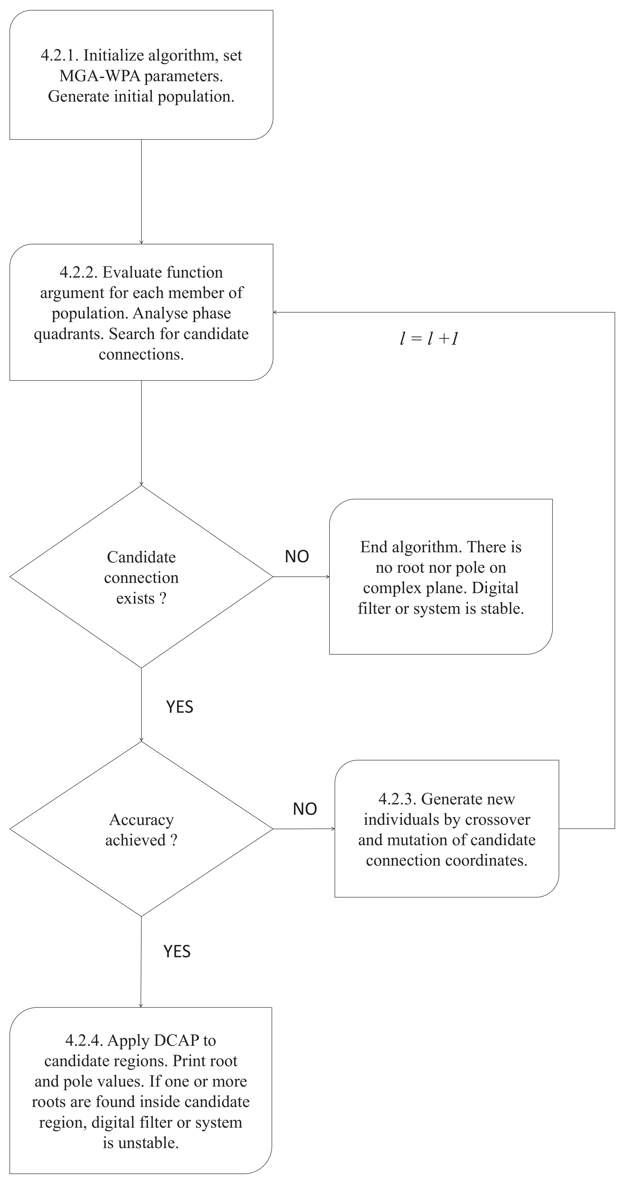
4.2. MGA-WPA Algorithm

Genetic algorithms (GAs) were originally proposed by Holland [28]. This approach employs a mathematical model of biological evolution to solve optimization problems. The original algorithm is based on binary operations on chromosomes of individuals (i.e., population members). The chromosomes are moved to a new population by genetic operators of selection, crossover, and mutation. The selection operator chooses from the population the chromosomes that are reproduced, the crossover operator exchanges parts of chromosomes between individuals, and the mutation operator changes alleles in chromosomes. A modification of the original GA, which operates in the continuous domain, is referred to as the breeder GA (BGA) [29]. Benchmarks indicate that BGAs outperform classical GAs in continuous search problems [30]. The crossover and mutation operators are main genetic operators for continuous functions. The mutation scheme generates new population members in a region defined by coordinates of a mutated individual and a mutation range. The crossover scheme generates new population members in a region between candidates with the most promising chromosomes. The BGA algorithm finds the single best solution of a fitness function but cannot deal with multimodal searching with multiple good solutions. Hence, the MGA-WPA algorithm was proposed in [23], which adapts BGA to solve problems of finding multiple zeros and poles. The proposed algorithm employs a set of rules allowing for population diversity and precise exploration of different regions on the complex plane. The population diversity stems from spatial separation of candidate regions. An individual either belongs to a candidate edge or not; thus, a new population is easily diversified and generated only in regions of zero or pole locations. The mutated or crossovered individuals are not replaced by new individuals; hence, the population size increases in each iteration of the algorithm. In this paper, we implement MGA-WPA to test stability of digital filters. A flowchart of the stability test with the MGA-WPA algorithm is presented in Figure 3. This algorithm is executed following those steps:

4.2.1. Algorithm Initialization and Generation of Initial Population Members

For its execution, the algorithm requires parameters such as the algorithm accuracy $ϵ$, the size of initial population N, the mutation range $R_M$, and the mutation precision $K_M$. Then, the uniformly distributed random population is generated inside the unit circle on the complex w-plane:

$$W=\{w_1,w_2,\dots ,w_N\}$$

(15)

where N is the initial population size.

4.2.2. Search for Regions in Vicinity of Zeros and Poles

For each individual population member, whose coordinates on the complex w-plane are denoted as $w_i$ ($i=1,2,\dots ,n_l$, where $n_l$ is the population size in the lth iteration), the complex-function argument and the associated phase quadrant (11) are evaluated. Then, Delaunay’s triangulation is applied to coordinates $w_i$, i.e., triangular connections between population members are generated. The phase-quadrant distance (12) along each of the connections is computed, and candidate connections are found. If there are neither zeros nor poles on the complex plane, candidate connections are not found and the algorithm execution is terminated. This means that the considered digital filter (or the system in general) is stable. If at least one candidate connection is found, then the candidate-connection length is computed. If the maximum length of collected candidate connections is smaller than the assumed accuracy, then the algorithm proceeds to the step described in Section 4.2.4. In other cases, the algorithm proceeds to the next step described in Section 4.2.3.

4.2.3. Crossover and Mutation of Population

New members of the population are generated by genetic operations of crossover and mutation. The genetic operations are executed on the coordinates of candidate connections. The crossover is executed on two individuals $w_i^{\prime }$ and $w_i^{″}$, which form the ith candidate connection. Then, the coordinates of a new individual resulting from the crossover are given by

$$\begin{array}{c}\hfill w_{n_l+i}=Re(w_i^{\prime }+a_i(w_i^{″}-w_i^{\prime }))\\ \hfill +jIm(w_i^{\prime }+b_i(w_i^{″}-w_i^{\prime }))\end{array}$$

(16)

where $i=1,2,\dots ,k_l$, $w_{n_l+i}$ denotes the coordinates of a new individual, $w_i^{\prime }$ denotes the coordinates of the first individual within the ith candidate connection, $w_i^{″}$ denotes the coordinates of the second individual within the ith candidate connection, $a_i$ and $b_i$ are random numbers between 0 and 1, and $k_l$ is the number of candidate connections detected in the lth iteration. The mutation operation is executed by mutating the coordinates of candidate-connection centres. Hence, the coordinates of new individuals resulting from the mutation are given by

$$\begin{array}{c}\hfill w_{n_l+k_l+i}=Re(s_i+{\Delta }_i{R}_M{c}_i{m}_i)+jIm(s_i+{\Delta }_i{R}_M{d}_i{m}_i)\end{array}$$

(17)

$$s_i=0.5(w_i^{\prime }+w_i^{″})$$

(18)

$${\Delta }_i=0.5|w_i^{\prime }-w_i^{″}|$$

(19)

$$m_i=2^{-u_i{K}_M}$$

(20)

where $i=1,2,\dots ,k_l$, $w_{n_l+k_l+i}$ denotes the coordinates of a new individual, $w_i^{\prime }$ denotes the coordinates of the first individual within the ith candidate connection, $w_i^{″}$ denotes the coordinates of the second individual within the ith candidate connection, $s_i$ denotes the coordinates of the ith candidate-connection centre, ${\Delta }_i$ denotes half of the length of the ith candidate connection, $c_i$ and $d_i$ are random numbers between $-1$ and 1, $R_M$ denotes the mutation range between 0 and 1, $u_i$ is a random number between 0 and 1, and $K_M$ denotes the mutation precision. As a result of the crossover and mutation operations, new population members are generated. The number of generated new individuals depends on the number of detected candidate connections. For each candidate connection, two individuals (i.e., one crossovered and one mutated) are generated. Hence, the population size $n_l$ is increased in each iteration based on the following formula:

$$n_{l+1}=n_l+2k_l.$$

(21)

In (21), $k_l$ denotes the number of candidates detected in the lth iteration. After the generation of new population members, the index l is increased and the algorithm is looped to the step consisting of searching for candidates, described in Section 4.2.2.

4.2.4. Stability Verification by Inspection of Candidate Regions

In the final step, the existence of zeros inside the unit circle is confirmed by using DCAP and Equation (14). If the parameter $q_k$ is a positive integer, then a function zero is found inside a candidate region and the considered system is unstable.

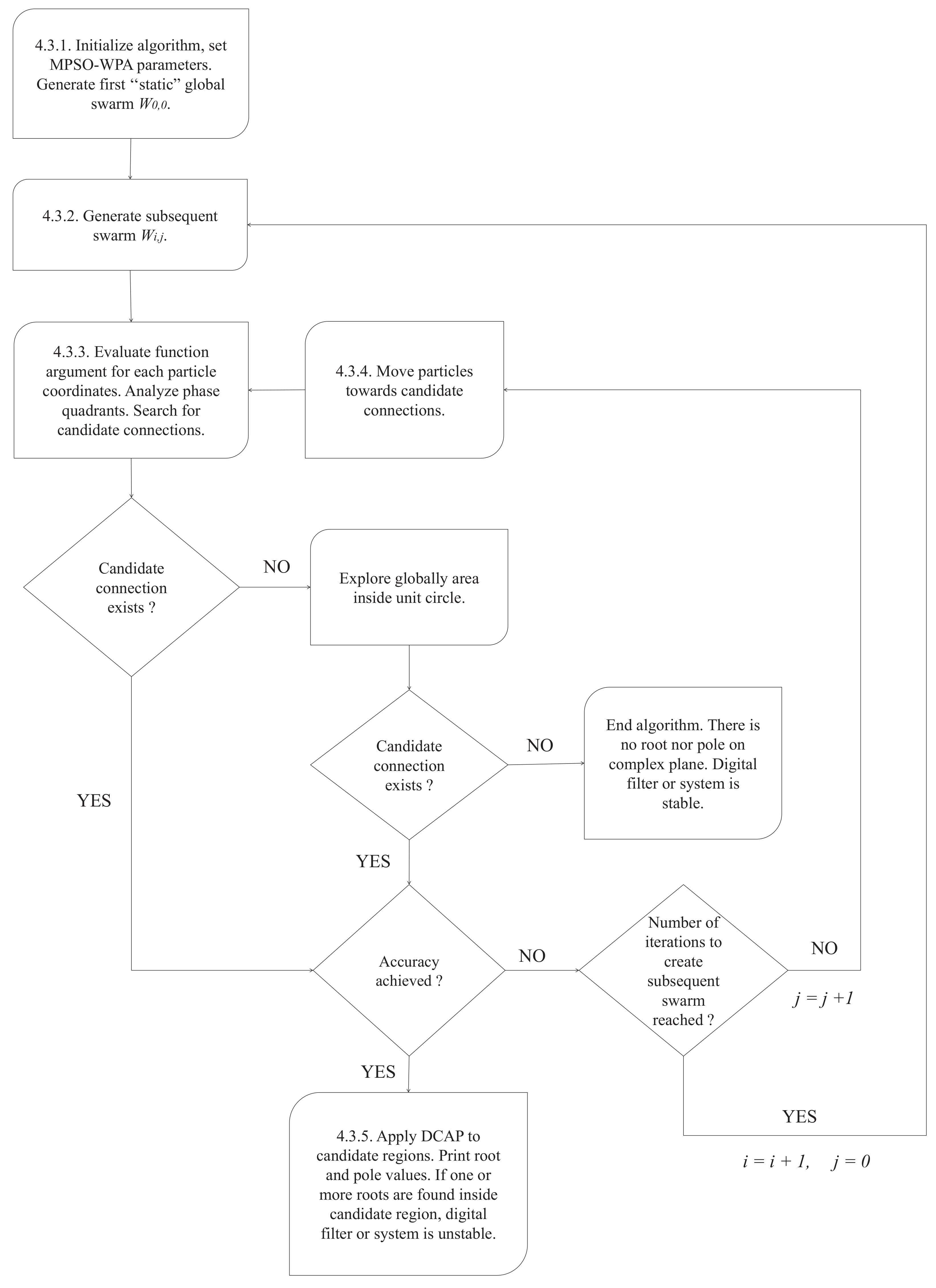
4.3. MPSO-WPA Algorithm

The algorithm of particle swarm optimization (PSO) was introduced by Kennedy and Eberhart [31]. It originated from the observed social and cooperative behavior of various intelligent colonies in nature. PSO, like GAs, is initialized with random population of nodes, called particles. The set of particles is defined as a swarm. Tracking of particle coordinates in space, which are associated with the best known solutions, and simultaneous sampling of the space while moving the population towards them are the basic principles of PSO operation. The most widely known variant of PSO [32] introduces inertia to the original formula as follows:

$$v_i=w{v}_i^{\prime }+c_1{u}_1(p_i-x_i)+c_2{u}_2(p_g-x_i)$$

(22)

$$x_i=x_i^{\prime }+v_i.$$

(23)

In (22) and (23), $v_i$ and $v_i^{\prime }$ are, respectively, current and previous velocities of the ith particle. The variables $p_i$ and $p_g$ are, respectively, the best coordinates found so far by an individual particle and the best coordinates found so far by a whole swarm. The scaling factors $c_1$ and $c_2$ represent, respectively, attractions towards the best position of the ith particle and the best position of the whole swarm. The parameters $u_1$ and $u_2$ are randomly generated numbers between 0 and 1. The inertia weight w determines how much the previous velocity is preserved. The particle coordinates $x_i$ are updated by adding velocity $v_i$ to the previous particle coordinates $x_i^{\prime }$. The original algorithm is dedicated to global-minimum searching and is not fully efficient when exploring multimodal functions. Multimodal optimization is focused on exploring a single function (from the characteristic equation in the case of filter-stability testing) to find multiple (most accurate) solutions, usually in different distant space regions. However, the original method suffers from premature convergence to a global solution because all particle velocities are updated in each iteration by $p_g$. This led to an uprise in new learning techniques that determine the information distribution between particles [33,34]. The swarm learning methods not only employ movement direction and velocity but also define how swarms are divided and distributed in search regions. It is extremely important, especially in the case of multimodal search, where regions of interest are distant from each other. MPSO-WPA [25] merges the PSO algorithm with the function-phase analysis to find roots and poles. In MPSO-WPA, the diversity of swarms stems from acceleration of the particles towards the nearest candidate connections. It allows for diversification of swarms and thorough exploration of regions of zero and pole locations. In this paper, we employ MPSO-WPA to test the stability of discrete-time LTI systems. A flowchart of the stability test applying the MPSO-WPA algorithm is presented in Figure 4. This numerical test is executed following those steps:

4.3.1. Algorithm Initialization and Generation of Initial Swarm

For its execution, the algorithm requires parameters such as the algorithm accuracy $ϵ$, the inertia weight g, the scaling factor s, the number of particles in swarms n, the number of swarm iterations L, and the initial velocity of particles. Next, a uniformly distributed random swarm (i.e., a set of particle coordinates) is generated within the unit circle on the complex w-plane:

$$W_{i,j}=\{w_{i,j,1},w_{i,j,2},\dots ,w_{i,j,n}\}$$

(24)

where i is the swarm number and j is the iteration number. The indices i and j are set to zero for the initial swarm. It is assumed that $W_{0,0}$ is not updated in subsequent iterations.

4.3.2. Generation of Subsequent Swarms

Next, the ith index is incremented and a subsequent, uniformly distributed swarm $W_{i,j}=\{w_{i,j,1},w_{i,j,2},\dots ,w_{i,j,n}\}$ is generated on the complex plane. The first swarm ($i=1$) is generated globally, and its role is to perform a wide-space search on the complex w-plane. If the ith index is greater than one, then such a swarm is divided into sub-swarms and generated locally only inside the candidate regions.

4.3.3. Search for Regions in Vicinity of Zeros and Poles

In this step, the function argument is evaluated for coordinates of each particle, and the phase quadrant in which the function value is located, is computed using (11). Then, Delaunay’s triangulation is applied to coordinates of all the particles, i.e., triangular connections between the particles are generated. Next, the phase-quadrant distance along each of the connections is computed using (12), and candidate connections can be found. If any candidate connection is not found, then the first swarm globally explores the unit circle by randomly changing the coordinates of its particles. If after L random changes of coordinates of particles in the first swarm no candidate connection is not found, then the algorithm returns information stating that the system is stable and exits. Otherwise, the coordinates of the centre of each candidate connection and its length are computed. If the maximum length of the collected candidate connections is smaller than the initially assumed accuracy, then the algorithm proceeds to the step described in Section 4.3.5. Otherwise, if the number of current iteration is equal to the number of swarm iterations L or its multiple, the algorithm executes the loop to the step described in Section 4.3.2 or proceeds to the next step described in Section 4.3.4.

4.3.4. Narrowing Candidate Regions

For each particle, the distances between its location and candidate-connection centres are computed. Then, again for each particle, the closest candidate-connection centre is determined and its coordinates are stored in the following set:

$$P_{i,j}=\{p_{i,j,1},p_{i,j,2},\dots ,p_{i,j,n}\}$$

(25)

where i is the swarm number and j is the iteration number. Next, each particle contained in the ith swarm is accelerated in the direction of its closest candidate centre by updating its velocity through vector operations:

$$V_{i,j+1}=g{V}_{i,j}+cu(P_{i,j}-W_{i,j})$$

(26)

where $V_{i,j}$ denotes the particle velocities; c denotes the scaling factor; g denotes the inertial weight, which determines how much the particle preserves its original direction of motion; and u denotes a random number between 0 and 1. Next, the coordinates of the ith swarm particles $W_{i,j}$ are updated by

$$W_{i,j+1}=W_{i,j}+V_{i,j+1}.$$

(27)

Then, the step consisting of searching for candidates, described in Section 4.3.3, is executed.

4.3.5. Stability Verification by Inspection of Candidate Regions

Finally, the existence of zeros inside the unit circle is confirmed by using DCAP and Equation (14). If the parameter $q_k$ is a positive integer, then a function zero is found inside a candidate region and the considered system is unstable.

5. Numerical Results

Numerical benchmarks were executed on a personal computer equipped with Intel i7-4700MQ processor. The codes for the stability tests were developed in Matlab. The characteristic equation, i.e., a function for which the roots (i.e., zeros) are investigated, and the algorithm parameters are the input data. The output data are values and multiplicities of the zeros and poles that have been found. Moreover, the code returns information on whether the considered system is stable or unstable. In the first test, the stability of integer-order digital filter is evaluated. Then, fractional-order systems are evaluated in terms of stability.

5.1. Integer-Order Digital Filter

Let us consider the digital filter [20] described by

$$H\left(z\right)=\frac{G}{A\left(z\right)}$$

(28)

where G is the gain factor and $A\left(z\right)$ is the characteristic-equation function defined by

$$\begin{array}{cc}\hfill A\left(z\right)=& +1.0000-2.5400z^{-1}+3.0429z^{-2}-2.9211z^{-3}\hfill \\ \hfill & +3.7088z^{-4}-3.9740z^{-5}+3.0221z^{-6}\hfill \\ \hfill & -2.3163z^{-7}+1.9791z^{-8}-1.1265z^{-9}\hfill \\ \hfill & +0.3855z^{-10}-0.2189z^{-11}+0.1171z^{-12}.\hfill \end{array}$$

(29)

For the filter stability, all the zeros of $A\left(z\right)$ must be located inside the unit circle. By applying the transformation (7), one obtains

$$\begin{array}{cc}\hfill A\left(w\right)=& +1.0000-2.5400w+3.0429w^2-2.9211w^3\hfill \\ \hfill & +3.7088w^4-3.9740w^5+3.0221w^6\hfill \\ \hfill & -2.3163w^7+1.9791w^8-1.1265w^9\hfill \\ \hfill & +0.3855w^{10}-0.2189w^{11}+0.1171w^{12}.\hfill \end{array}$$

(30)

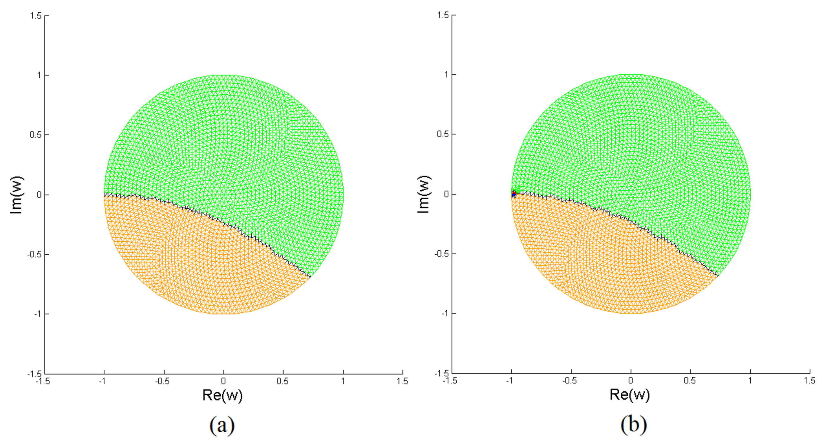
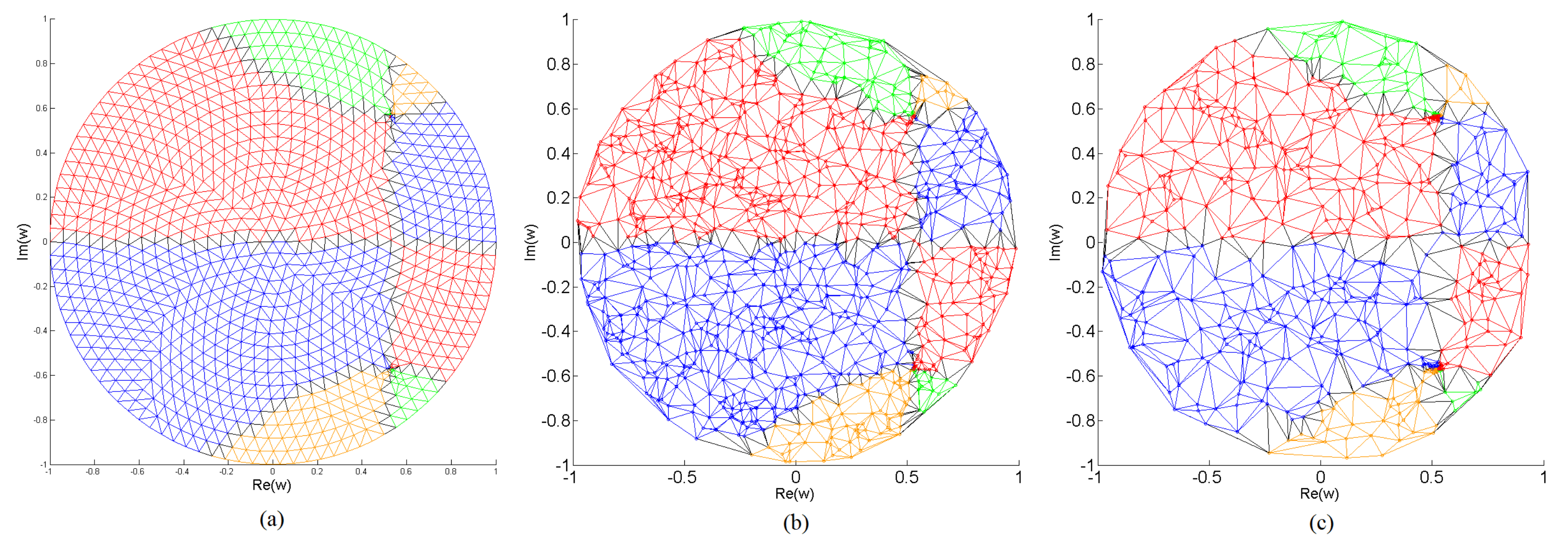
The stability test for GRPF is executed with the mesh resolution $r=0.07$. Hence, the initial number of generated nodes is equal to 919. To obtain comparable results, the benchmarks for MGA-WPA and MPSO-WPA are also executed with the same initial number of individuals or particles, respectively. The accuracy of the algorithms is set to $\epsilon ={10}^{-5}$. The final distributions of nodes with Delaunay’s triangulations for exemplary runs of GRPF, MGA-WPA, and MPSO-WPA are presented in Figure 5. The tested filter is unstable because all the algorithms find two conjugate zeros inside the unit circle:

$$w=0.829238\pm 0.536757j.$$

The stability test lasts 0.15 s for GRPF, 0.3 s for MGA-WPA, and 0.23 s for MPSO-WPA. The GRPF algorithm executes 14 iterations and generates 1080 nodes in total. The MGA-WPA algorithm executes 17 iterations and generates 1033 individuals in total. The MPSO-WPA algorithm executes 11 iterations and generates 1019 particles in total. The computing times and final numbers of nodes for GRPF, MGA-WPA, and MPSO-WPA are presented in

Table 1. Computing times and numbers of generated nodes in the stability tests of a considered integer-order digital filter.

Method	Computing Time (s)	Nodes
GRPF	0.15	1080
MGA-WPA	0.3	1033
MPSO-WPA	0.23	1019

.

It is worth mentioning that the zeros located very close to the unit circle are difficult to compute because the quadrant distances are computed only between the particles located inside the unit circle. In consequence, a function zero located close to the unit circle may be missed. In order to avoid such a situation, the number of generated nodes may be increased to collect more phase samples of the complex function, especially at the points located close to the unit circle. Another solution is to increase the size of the search region, e.g., by considering the region $\left|w\right|<1.1$ and by verifying if the detected zero is positioned within the unit circle. In our opinion, a more reliable and less computationally demanding approach is to increase the w-plane search region.

5.2. High-Order Systems

Stability tests of high-order systems are computationally demanding because a large number of zeros complicates the phase portrait of the complex function in the characteristic equation. It may lead to false detection of candidate regions and to exploration of irrelevant regions by the algorithms. Let us consider a system for which the characteristic equation is given by the function

$$f\left(z\right)=(z-2)\prod _{i=1}^L[z-{(-1)}^{i}0.4(1+\frac{i}{L})].$$

(31)

As one can notice, the system is unstable because a single zero of such a characteristic equation is located outside the unit circle on the complex z-plane ($z=2$). The characteristic equation is mapped onto the w-domain. Although the algorithms that utilize the phase analysis do not need to remove singularities from a complex function, in this benchmark, singularities are removed according to (8) due to long computing times. The stability tests are executed for the accuracy set to $\epsilon ={10}^{-5}$. The initial number of generated nodes is set to 919. With the increase in parameter L, the phase portrait of the characteristic function $F\left(w\right)$ becomes more and more complicated. If only 919 nodes are generated initially, the GRPF method is not able to converge when the system order is set at 80 and higher. A more dense initial mesh is required to overcome this limitation. However, MGA-WPA and MPSO-WPA usually converge for a system order higher than 80 in our benchmarks. The number of finally generated nodes and the times necessary for the convergence (i.e., computing times), when the system order is varied, are presented in

Table 2. Computing times and numbers of generated nodes in stability tests of considered high-order systems.

Method	L	Computing Time (s)	Nodes
GRPF	1	0.17	1312
	5	0.18	1312
	10	0.19	1315
	20	0.20	1315
	40	0.23	1343
MGA-WPA	1	0.24	965
	5	0.20	961
	10	0.21	973
	20	0.22	969
	40	0.25	1055
	80	0.52	1901
	100	0.95	2785
MPSO-WPA	1	0.23	1019
	5	0.24	1019
	10	0.24	1019
	20	0.61	1519
	40	0.97	1720
	80	3.06	2956
	100	4.34	3334

.

The algorithms are fast and efficient for low-order systems, i.e., for low values of the L parameter. However, in the case of a complicated phase portrait of the considered complex function, the algorithms require longer times and a large number of nodes to converge for the assumed accuracy. The distributions of nodes with Delaunay’s triangulations in final iterations for the system (31) when $L=40$, with singularities removed, are presented in Figure 6.

5.3. Fractional-Order Digital Filter

Let us consider the fractional-order digital filter described by the transfer function:

$$H\left(z\right)=\frac{1}{{\left(\frac{2}{T}\frac{1-z^{-1}}{1+z^{-1}}\right)}^{\alpha +\beta }+a{\left(\frac{1-z^{-1}}{1+z^{-1}}\right)}^{\alpha }+c}$$

(32)

where a and c are the design parameters, $\alpha$ and $\beta$ are the fractional-order parameters, and T is the sampling period. The characteristic equation of the filter in the w-domain is given by

$$F\left(w\right)=s^{(\alpha +\beta )}+a{s}^{\alpha }+c$$

(33)

where

$$s=\frac{2(1-w)}{T(1+w)}.$$

(34)

The pole $w=-1$ can be removed; hence, the stability is tested based on the following equation:

$$F\left(w\right){(1+w)}^{\alpha +\beta }=0.$$

(35)

Let us assume that $\alpha =\beta =0.5$, $a=1$, $c=-1000+50j$, and $T=0.001$. The initial number of generated nodes for all the methods is set to 919. The algorithm accuracy is set to $\epsilon ={10}^{-5}$. The final distributions of nodes with Delaunay’s triangulations for exemplary runs of GRPF, MGA-WPA, and MPSO-WPA are presented in Figure 7. The tested filter is unstable because all the algorithms found a single root inside the unit circle:

$$w=0.346947+0.022324j.$$

In exemplary runs, the stability test lasts 0.15 s for GRPF, 0.18 s for MGA-WPA, and 0.20 s for MPSO-WPA. The GRPF algorithm executes 14 iterations and generates 993 nodes in total. The MGA-WPA algorithm executes 15 iterations and generates 962 individuals in total. The MPSO-WPA algorithm executes 8 iterations and generates 1019 particles in total. The computing times and final numbers of nodes for the GRPF, MGA-WPA, and MPSO-WPA methods are presented in

Table 3. Computing times and numbers of generated nodes in the stability tests of the considered fractional-order digital filter.

Method	Computing Time (s)	Nodes
GRPF	0.15	993
MGA-WPA	0.18	962
MPSO-WPA	0.20	1019

.

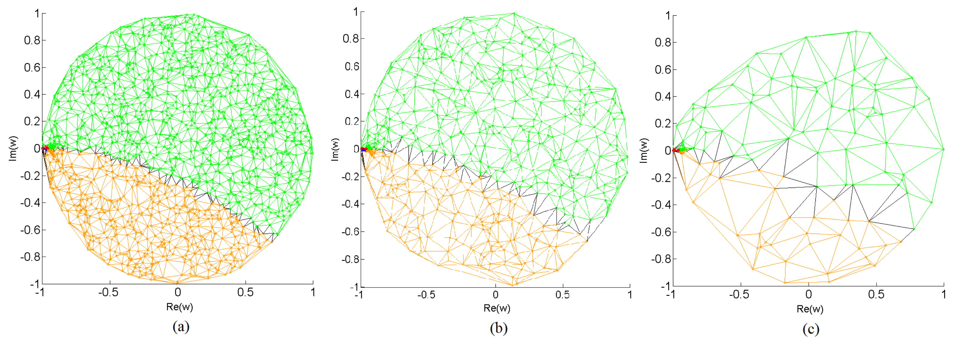
Let us consider another computationally difficult case. The fractional-order digital filter (32) is now considered for the parameters $\alpha =\beta =0.5$, $a=1$, $c=-1000-100j$, and $T=0.01$. The pole $w=-1$ is not extracted in order to obtain an “island”-like phase portrait of the considered function. Empirical tests show that the mesh size must be smaller than or equal to $r=0.039$ in order to detect the digital-filter instability (i.e., to find a zero inside the unit circle on the w-plane) using the GRPF method. Therefore, the algorithm must generate the mesh, which consists of more than 2971 nodes to detect the filter instability. The mesh with a smaller number of nodes causes the algorithm to miss the function zero located inside the unit circle and returns false information that the digital filter is stable. The distributions of nodes with Delaunay’s triangulations for the mesh sizes $r=0.04$ (2971 nodes) and $r=0.039$ (2977 nodes) are presented in Figure 8. The failure of the GRPF-based stability test for the considered fractional-order digital filter is presented in Figure 8a.

The GRPF method is not based on a stochastic generator such as MGA-WPA and MPSO-WPA; hence, its multiple executions always return the same test results. Only increasing the mesh density allows one to detect the digital-filter instability in the case of the first failure. On the other hand, MGA-WPA and MPSO-WPA are stochastic methods. The convergence process is different in each run; hence, multiple algorithm executions may allow one to detect the filter instability properly after a few failures. To benchmark MGA-WPA and MPSO-WPA, the detectability of an unstable zero for a varying number of initial nodes is tested for each algorithm in 5 runs. The random distribution of nodes in each run for MGA-WPA allows one to detect instability properly, even with a small number of initial nodes such as 250. With a small number of nodes, the algorithm avoids spending computing time on a function-phase analysis in redundant nodes. However, a reduced number of nodes increases the probability of stability-test failure. A trade-off must be carefully established between the number of nodes and the risk of failure at the algorithm’s first iteration.

Table 4. Initial number of individuals (nodes) and number of runs with correctly detected zeros for the MGA-WPA method. The stability test is executed 5 times for each number of nodes. A faultless run means that the filter instability is detected (zero is found inside the w-plane unit circle).

Nodes	Faultless Runs
2977	5
2500	3
2000	4
1500	2
1000	3
500	1
250	1

presents the number of runs with correctly detected filter instability for the MGA-WPA method as a function of the number of initial nodes. The distributions of nodes in the last iteration with Delaunay’s triangulations for a varying number of nodes for MGA-WPA algorithm initialization are presented in Figure 9.

The stability test executed with MPSO-WPA returns even more interesting results. MPSO-WPA takes advantage of swarm intelligence and involves global searching, which prevents missing zeros/poles on the complex plane. If a candidate connection is not detected in the first iteration, the MPSO-WPA algorithm uses the next swarm by randomly changing its positions to search for the missed zeros and poles. In consequence, the zero detection occurs 4 and 2 times more often compared to MGA-WPA for 500 and 250 initial nodes respectively. These results show clearly that, in the situation in which a small number of nodes is generated at algorithm initialization, MPSO-WPA is less likely to miss zeros/poles than MGA-WPA. It allows one to significantly reduce the number of nodes generated at the algorithm initialization and hence to reduce computation time.

Table 5. Number of particles (nodes) in the initial and first swarms and number of runs with correctly detected digital-filter instability for the MPSO-WPA method. The stability tests are executed 5 times for each number of nodes.

Nodes in Initial Swarm	Nodes in First Swarm	Faultless Runs
2477	500	5
2000	500	5
1500	500	5
1000	500	5
500	500	5
250	250	4
100	150	2

presents the numbers of runs with correctly detected filter instabilities for MPSO-WPA with a varying number of nodes in the initial and first swarms. The distributions of nodes with Delaunay’s triangulations in the last iteration for a varying number of nodes at MPSO-WPA initialization are presented in Figure 10.

5.4. Fractional-Order System

The presented methods can be applied to test the stability of various discrete-time systems, also of those described by the fractional-order state-space equations [4,5]:

$$\begin{array}{c}\hfill {\Delta }^{\alpha }\mathbf{x}(n+1)={\mathbf{A}}_f\mathbf{x}\left(n\right)+\mathbf{B}\mathbf{u}\left(n\right)\\ \hfill \mathbf{y}\left(n\right)=\mathbf{C}\mathbf{x}\left(n\right)+\mathbf{D}\mathbf{u}\left(n\right)\end{array}$$

(36)

where $\alpha$ is the fractional order and ${\mathbf{A}}_f=\mathbf{A}-\mathbf{I}$ is the difference between the discrete-time state-space system matrix $\mathbf{A}$ and the identity matrix $\mathbf{I}$. In (36), the fractional difference is defined as

$${\Delta }^{\alpha }x\left(n\right)=\sum _{j=0}^n{(-1)}^j\left(\genfrac{}{}{0pt}{}{\alpha }{j}\right)q^{-j}x\left(n\right)$$

(37)

where $q^{-1}$ is the backward shift operator.

Let us consider the fractional-order system represented by the matrix

$${\mathbf{A}}_f=\left[\begin{array}{cc}0.6& -1.45\\ 1& -1\end{array}\right].$$

(38)

For the systems (36) and (38), the characteristic equation is given by

$$f\left(z\right)=det[z{(1-z^{-1})}^{\alpha }\mathbf{I}-{\mathbf{A}}_f]=0.$$

(39)

By applying the transformation (7) and by multiplying by $w^2$, one obtains

$$F\left(w\right)=w^{2}f\left(w\right)={(1-w)}^{2\alpha }+0.4w{(1-w)}^{\alpha }+0.85w^2.$$

(40)

The stability tests are executed for the parameter $\alpha =1.1$. The accuracy of algorithms is set to $\epsilon ={10}^{-5}$. The number of initially generated nodes is set to 919. The final distributions of nodes with Delaunay’s triangulations for GRPF, MGA-WPA, and MPSO-WPA are presented in Figure 11.

Each of the benchmarked methods returns information stating that the system is unstable and finds two conjugate zeros inside the unit circle:

$$w=0.529268\pm 0.569170j.$$

(41)

The stability test based on GRPF generates 1068 nodes and lasts 0.16 s. The test based on MGA-WPA generates 1005 individuals and lasts 0.36 s. The MPSO-WPA method generates 1019 particles and lasts 0.2 s. The computation times and final numbers of nodes for the GRPF, MGA-WPA, and MPSO-WPA methods are summarized in

Table 6. Convergence times and final numbers of nodes for the GRPF, MGA-WPA, and MPSO-WPA methods for the stability test of a fractional-order system.

Method	Computation Time (s)	Nodes
GRPF	0.16	1068
MGA-WPA	0.36	1005
MPSO-WPA	0.20	1019

.

6. Discussion

The recently published methods for finding roots and poles, i.e., GRPF, MGA-WPA, and MPSO-WPA, are based on Delaunay’s triangulation and the function phase analysis. The main difference between the algorithms stems from the method of node generation and the enhancement of node density in the vicinity of roots and poles. The GRPF algorithm initially generates a regular triangular mesh of nodes. Then, the mesh becomes denser in the regions where roots and poles might be located. MGA-WPA generates a uniformly distributed random population and uses genetic operations to create new individuals in the vicinity of roots and poles. MSPO-WPA generates uniformly distributed random swarms consisting of particles and moves them towards roots and poles. The considered algorithms generate nodes that are differently located. Hence, in order to fairly compare the performance of these methods, a few assumptions must be made. Firstly, the accuracy of algorithms $\epsilon$, denoting the decimal-point precision of the root and pole computations, must be equal. Secondly, to compare the total number of function evaluations and the time necessary to converge, each algorithm must be initiated with the same number of nodes. The GRPF method generates a regular triangular mesh of nodes. The number of generated nodes depends on the parameter r and on the size of the search region. For $r=0.1$, $r=0.05$, and $r=0.01$, this algorithm generates, respectively, 547, 1801, and 40,717 nodes inside the unit circle. The number of initially generated nodes is set directly by a user for MGA-WPA and MPSO-WPA. Meshing is another problem in algorithm comparison because it can result in two common issues. The first one is related to the failure of root or pole detection, especially when roots and poles are located close to each other and create an “island”-like region. The second issue is related to the mesh geometry around the unit circle, which may cause computational issues when a root/pole is located close to the unit circle. Increasing the mesh density around the unit circle can be a solution to this problem. However, meshing that involves a high number of nodes also has a drawback. That is, the function phase must be evaluated in each node, which increases the execution time of the algorithm. Therefore, the trade-off between the number of generated nodes and the execution time should be established according to the considered characteristic equation. The benchmarks clearly show that, if computing time is not vitally important for the user, MPSO-WPA is the right choice, as it prevents missing zeros/poles. However, the GRPF or MGA-WPA methods are the right choice in the case of characteristic equations with simple phase portraits and without “island”-like regions. These methods do not generate redundant nodes, in contrast to MPSO-WPA, to overcome missing zeros/poles and consequently require fewer computing resources and less time. It is worth mentioning that MGA-WPA requires, on average, fewer nodes than GRPF to find a solution with a given accuracy. On the other hand, the computing time of GRPF method is shorter in comparison to MGA-WPA. However, this shorter computing time stems mainly from the higher number of nodes generated in each algorithm loop. The mesh refinement algorithm of GRPF creates extra nodes in the centres of the edges in candidate regions. Hence, for each detected candidate connection, five new nodes are generated (i.e., one in the centre of the candidate edge and four in the centres of edges that form the candidate-region boundary). The MGA-WPA algorithm generates two nodes for each detected candidate connection (i.e., the first one from crossover and the second one from mutation). In consequence, MGA-WPA algorithm is slower because it iterates the algorithm loop executing Delaunay’s triangulation more frequently.

7. Conclusions

The GRPF, MGA-WPA, and MPSO-WPA methods for stability testing of digital filters are presented and benchmarked in this paper. The methods evaluate the stability of integer- and fractional-order digital filters and systems. The algorithms merge optimization techniques with phase analysis on the complex plane. The results obtained with the use of the algorithms are satisfactory. The tested algorithms are very fast in most cases. If either the digital filter or the system includes only a few zeros or poles and the phase portrait is not complicated, computations take a fraction of a second. In the presented cases, the longest stability test for a digital filter with two zeros located inside the unit circle on the complex w-plane lasts 0.36 s. Even for a high-order system (order set to 100), with a complicated phase portrait, the computation time rises up to 0.95 s for MGA-WPA and 4.34 s for MPSO-WPA. The algorithms do not require singularities to be removed from the considered complex functions. However, testing stability without removing singularities as well as testing stability of high-order systems may be computationally inefficient for functions with complicated phase portraits. It is worth noticing that each algorithm has slightly different properties. GRPF is very fast and efficient; however, it requires an initial number of nodes to be large enough to detect all candidate edges. In the exemplary benchmark of GRPF, it is necessary to generate as many as 2971 initial nodes to detect the fractional-order digital filter instability. However, MGA-WPA and MPSO-WPA allow for detecting digital filter instability using only 250 nodes generated at the algorithm initialization. For MGA-WPA, a small number of individuals is sufficient for the convergence, limiting the final population size. Furthermore, the MGA-WPA method may not find any root or pole if the initial population members are separated by a large distance. However, the stochastic nature of MGA-WPA increases the probability of finding all roots and poles when the algorithm is executed multiple times. MPSO-WPA also prevents missing roots and poles due to the usage of stochastic space exploration by subsequent swarms; however, such an algorithm that prevents missing zeros/poles requires high computing time. These properties lead to the conclusion that stochastic-based methods such as MGA-WPA and MPSO-WPA are more likely to detect system instability, especially when run multiple times. If the computing time is not important for the user, MPSO-WPA is the right choice, as it prevents missing zeros/poles. If computing time is important and “island”-like regions are not expected to occur on the complex w-plane inside the unit circle, it is recommended that either MGA-WPA or GRPF is used.

References

- Ogata, K. Discrete-Time Control Systems; Prentice-Hall International: Upper Saddle River, NJ, USA, 1995. [Google Scholar]
- Oppenheim, A.; Schafer, R.W.; Buck, J.R. Discrete-Time Signal Processing; Prentice-Hall International: Upper Saddle River, NJ, USA, 1999. [Google Scholar]
- Jury, E.I. Theory and Application of the Z-Transform Method; John Wiley and Sons: Hoboken, NJ, USA, 1964. [Google Scholar]
- Stanisławski, R.; Latawiec, K.J. Stability analysis for discrete-time fractional-order LTI state-space systems. Part I: New necessary and sufficient conditions for the asymptotic stability. Bull. Pol. Acad. Sci. Tech. Sci. 2013, 61, 353–361. [Google Scholar] [CrossRef] [Green Version]
- Stanisławski, R.; Latawiec, K.J. Stability analysis for discrete-time fractional-order LTI state-space systems. Part II: New stability criterion for FD-based systems. Bull. Pol. Acad. Sci. Tech. Sci. 2013, 61, 363–370. [Google Scholar] [CrossRef]
- Kravanja, P.; Sakurai, T.; van Barel, M. On Locating Clusters of Zeros of Analytic Functions. BIT Numer. Math. 1999, 39, 646–682. [Google Scholar] [CrossRef]
- Kravanja, P.; van Barel, M.; Ragos, O.; Vrahatis, M.; Zafiropoulos, F. ZEAL: A mathematical software package for computing zeros of analytic functions. Comput. Phys. Commun. 2000, 124, 212–232. [Google Scholar] [CrossRef]
- Meylan, M.H.; Gross, L. A parallel algorithm to find the zeros of a complex analytic function. ANZIAM J. 2003, 44, E236–E254. [Google Scholar] [CrossRef] [Green Version]
- Gillan, C.; Schuchinsky, A.; Spence, I. Computing zeros of analytic functions in the complex plane without using derivatives. Comput. Phys. Commun. 2006, 175, 304–313. [Google Scholar] [CrossRef]
- Yu-Bo, T. Solving Complex Transcendental Equations Based on Swarm Intelligence. IEEJ Trans. Electr. Electron. Eng. 2009, 4, 755–762. [Google Scholar] [CrossRef]
- Ariyaratne, M.K.A.; Fernando, T.G.I.; Weerakoon, S. A self-tuning modified firefly algorithm to solve univariate nonlinear equations with complex roots. In Proceedings of the 2016 IEEE Congress on Evolutionary Computation (CEC), Vancouver, BC, Canada, 24–29 July 2016; pp. 1477–1484. [Google Scholar]
- Zadehgol, A. A frequency-independent and parallel algorithm for computing the zeros of strictly proper rational transfer functions. Appl. Math. Comput. 2016, 274, 229–236. [Google Scholar] [CrossRef]
- Chen, P.Y.; Sivan, Y. Robust location of optical fiber modes via the argument principle method. Comput. Phys. Commun. 2017, 214, 105–116. [Google Scholar] [CrossRef] [Green Version]
- Zouros, G.P. CCOMP: An efficient algorithm for complex roots computation of determinantal equations. Comput. Phys. Commun. 2018, 222, 339–350. [Google Scholar] [CrossRef]
- Michalski, J.J. Complex Border Tracking Algorithm for Determining of Complex Zeros and Poles and its Applications. IEEE Trans. Microw. Theory Technol. 2018, 66, 5383–5390. [Google Scholar] [CrossRef]
- Ostalczyk, P. Equivalent Descriptions of a Discrete-Time Fractional-Order Linear System and Its Stability Domains. Int. J. Appl. Math. Comput. Sci. 2012, 22, 533–538. [Google Scholar] [CrossRef] [Green Version]
- Stanisławski, R.; Latawiec, K.J. A modified Mikhailov stability criterion for a class of discrete-time noncommensurate fractional-order systems. Commun. Nonlinear Sci. Numer. Simul. 2021, 96, 105697. [Google Scholar] [CrossRef]
- Grzymkowski, L.; Trofimowicz, D.; Stefanski, T.P. Stability Analysis of Interconnected Discrete-Time Fractional-Order LTI State-Space Systems. Int. J. Appl. Math. Comput. Sci. 2020, 30, 649–658. [Google Scholar]
- Grzymkowski, L.; Stefanski, T.P. Numerical Test for Stability Evaluation of Discrete-Time Systems. In Proceedings of the 2018 23rd International Conference on Methods Models in Automation Robotics (MMAR), Międzyzdroje, Poland, 27–30 August 2018; pp. 803–808. [Google Scholar]
- Grzymkowski, L.; Stefanski, T.P. A New Approach to Stability Evaluation of Digital Filters. In Proceedings of the 2018 25th International Conference “Mixed Design of Integrated Circuits and System” (MIXDES), Gdynia, Poland, 21–23 June 2018; pp. 351–354. [Google Scholar]
- Kowalczyk, P. Complex Root Finding Algorithm Based on Delaunay Triangulation. ACM Trans. Math. Softw. 2015, 41, 1–13. [Google Scholar] [CrossRef]
- Kowalczyk, P. Global Complex Roots and Poles Finding Algorithm Based on Phase Analysis for Propagation and Radiation Problems. IEEE Trans. Antennas Propag. 2018, 66, 7198–7205. [Google Scholar] [CrossRef]
- Trofimowicz, D.; Stefański, T.P. Multimodal Genetic Algorithm with Phase Analysis to Solve Complex Equations of Electromagnetic Analysis. In Proceedings of the 2020 23rd International Microwave and Radar Conference (MIKON), Warsaw, Poland, 5–7 October 2020; pp. 24–29. [Google Scholar]
- Trofimowicz, D.; Stefański, T.P. Testing Stability of Digital Filters Using Multimodal Particle Swarm Optimization with Phase Analysis. In Proceedings of the 2020 27th International Conference on Mixed Design of Integrated Circuits and System (MIXDES), Łódź, Poland, 25–27 June 2020; pp. 232–236. [Google Scholar]
- Trofimowicz, D.; Stefański, T.P. Multimodal Particle Swarm Optimization with Phase Analysis to Solve Complex Equations of Electromagnetic Analysis. In Proceedings of the 2020 23rd International Microwave and Radar Conference (MIKON), Warsaw, Poland, 5–7 October 2020; pp. 44–48. [Google Scholar]
- Krantz, S.G. Handbook of Complex Variables, 1st ed.; Birkhäuser: Boston, MA, USA, 1999. [Google Scholar]
- Duren, P.; Hengartner, W.; Laugesen, R.S. The Argument Principle for Harmonic Functions. Am. Math. Mon. 1996, 103, 411–415. [Google Scholar] [CrossRef]
- Holland, J.H. Adaptation in Natural and Artificial Systems; MIT Press: Cambridge, MA, USA, 1975. [Google Scholar]
- Mühlenbein, H.; Schlierkamp-Voosen, D. Predictive Models for the Breeder Genetic Algorithm I. Continuous Parameter Optimization. Evol. Comput. 1993, 1, 25–49. [Google Scholar] [CrossRef]
- Falco, I.D.; Balio, R.D.; Cioppa, A.D.; Tarantino, E. A Comparative Analysis of Evolutionary Algorithms for Function Optimisation. In Proceedings of the 2nd Workshop on Evolutionary Computing (WEC2), Nagoya, Japan, 4–22 March 1996; pp. 29–32. [Google Scholar]
- Eberhart, R.C.; Kennedy, J. A new optimizer using particle swarm theory. In Proceedings of the Sixth International Symposium on Micro Machine and Human Science, Nagoya, Japan, 4–6 October 1995; Volume 1, pp. 39–43. [Google Scholar]
- Shi, Y.; Eberhart, R. A modified particle swarm optimizer. In Proceedings of the IEEE Congress on Evolutionary Computation, Anchorage, AK, USA, 4–9 May 1998; pp. 69–73. [Google Scholar]
- Liang, J.J.; Qin, A.K.; Suganthan, P.N.; Baskar, S. Comprehensive learning particle swarm optimizer for global optimization of multimodal functions. IEEE Trans. Evol. Comput. 2006, 10, 281–295. [Google Scholar] [CrossRef]
- Zhan, Z.; Zhang, J.; Li, Y.; Shi, Y. Orthogonal Learning Particle Swarm Optimization. IEEE Trans. Evol. Comput. 2011, 15, 832–847. [Google Scholar] [CrossRef] [Green Version]
Figure 1.
Triangulated area inside the unit circle for function and . Zeros are located at . The candidate edges () are between nodes 2–4, 6–9, and 7–9. The zeros are located inside contours 1–2–3–4 () and 5–6–7–8–9 (). The boundary of candidate regions consists of cyan lines (–). Quadrants of w-plane: • Q = 1, • Q = 2, • Q = 3, and • Q = 4.
Figure 2.
Flowchart of stability test with the global complex roots and poles finding (GRPF) algorithm.
Figure 3.
Flowchart of stability test with the multimodal genetic algorithm with phase analysis (MGA-WPA).
Figure 4.
Flowchart of stability test with the multimodal particle swarm optimization with phase analysis (MPSO-WPA) algorithm.
Figure 5.
Distribution of nodes with Delaunay’s triangulation in the final iteration for (a) the GRPF, (b) MGA-WPA, and (c) MPSO-WPA methods. The stability tests of integer-order digital filter are executed in the transformed region . Phase quadrants of mesh nodes on the w-plane: • Q = 1, • Q = 2, • Q = 3, and • Q = 4.
Figure 6.
Distribution of nodes with Delaunay’s triangulation in final iteration for (a) the GRPF, (b) MGA-WPA, and (c) MPSO-WPA methods. The stability tests of a high-order system with are executed in the transformed region . Phase quadrants of mesh nodes on the w-plane: • Q = 1, • Q = 2, • Q = 3, and • Q = 4.
Figure 7.
Distribution of nodes with Delaunay’s triangulation in final iteration for (a) the GRPF, (b) MGA-WPA, and (c) MPSO-WPA methods. The stability tests of a fractional-order digital filter are executed in the transformed region . Phase quadrants of mesh nodes on the w-plane: • Q = 1, • Q = 2, • Q = 3, and • Q = 4.
Figure 8.
Distribution of nodes with Delaunay’s triangulation for the stability test of a fractional-order digital filter with the use of GRPF for mesh size (a) and (b) . A single zero is not detected for mesh size because it is not dense enough. Phase quadrants of mesh nodes on the w-plane: • Q = 1, • Q = 2, • Q = 3, and • Q = 4.
Figure 9.
Distribution of nodes with Delaunay’s triangulation for the stability test of a fractional-order digital filter with the use of MGA-WPA. The stability test results are presented for an initial number of nodes set to (a) 2000, (b) 1000, and (c) 250. The “island”-like region with unstable zero is detected. Phase quadrants of individuals on the w-plane: • Q = 1, • Q = 2, • Q = 3, and • Q = 4.
Figure 10.
Distribution of nodes with Delaunay’s triangulation for the stability test of a fractional-order digital filter with the use of MPSO-WPA. The results of the stability tests are presented for a number of nodes in the initial and first swarms set, respectively, to (a) 1500 and 500, (b) 500 and 500, and (c) 100 and 150 nodes. The “island”-like region with unstable zero is detected. Phase quadrants of particles on the w-plane: • Q = 1, • Q = 2, • Q = 3, and • Q = 4.
Figure 11.
Distribution of nodes with Delaunay’s triangulation in final iteration for (a) the GRPF, (b) MGA-WPA and (c) MPSO-WPA methods. The stability tests of a fractional-order system are executed in the transformed region . Phase quadrants of mesh nodes on the w-plane: • Q = 1, • Q = 2, • Q = 3, and • Q = 4.