Improving the Reliability of an Electric Power System by Biomass-Fueled Gas Engine

Abstract

This paper shows a practice to raise the reliability of an electric power system by the installation of distributed generation, taking gasified biomass as fuel. To calculate the reliability index, a probabilistic load flow was used. This index is determined as the fault probability of the system. The resolution of this probabilistic load flow combines the method of cumulants and Gram–Charlier expansion. To achieve the reliability index, simulating a number of contingencies is required; the greater the number of simulated contingencies, the higher the accuracy of the index obtained. This probabilistic technique uses the random variables as starting information, so the two generators and loads are simulated as random variables. The generators of this distributed generation are biomass-fueled gas engines, commonly found in Spain. The simulations carried out on the IEEE 14-bus Test System, including three biomass generators, show that the inclusion of this type of generation improves the overall reliability indices of the electrical system.

1. Introduction

Today’s electrical power systems have shown an unknown and veering behavior, either in terms of consumer demand or in the faults of their components. By simulating the incoming data as random variables in the issue, it is possible to identify the sources of uncertainties in the system.

Probabilistic load flow is the name of the load flow issue that uses random variables as input [1]. To calculate the load flow issue, different methodologies exist that take these random variables as initial data. There are certain analytical methods that work directly with random variables. Moreover, simulation methods exist that still employ deterministic algorithms to solve the issue, such as the Monte Carlo approach.

Through all the different simulation methods in the present day, the Monte Carlo approach has priority; this technique is capable of applying the procedure of deterministic load flows that have been previously created [2].

Numerous analytical techniques, including the point estimate approach [3] and the method of cumulants [4,5], can be used to solve the probabilistic load flow issue. These techniques employ the convolution characteristics of the random values and expect power flow through the lines and the power supplied at the buses, in order to determine the voltage also as random variables.

According to [6], for the cumulants procedure and [7] for the point estimate process, the major benefit of utilizing some of these approaches is their computational effectiveness when processing random variables.

Power system reliability is becoming crucial for the reform of the electrical sector [8]. Nowadays, the electric power system is configured as independent producers that supply energy to distributors across the existing transmission networks.

Frequently, the system administrator intends to amplify the power network with high-quality, and therefore costly, producers’ units to satisfy the conditions of system reliability as a consequence of the security requirements.

A huge number of factors influence the measurement of the reliability of the system, creating a laborious issue to be solved. This is conditioned by human creation factors: the readiness of power plants, level of loads at the buses, contingencies such as buses or lines out of service, and also, by natural unexpected/inevitability factors: hour of the day, day of the week, weather or season. In the methods discussed above, the random variables will be the estimated load and the availability of power plants, and both are essential aspects of an electric power system.

This article describes a method based on cumulants for enhancing a power system’s overall reliability. The aim of the issue is to establish minimum rates of the reliability index in the power system and increase them using distributed generation. The likelihood of a system failing, the frequency of failures, and the predicted length of time of the failure are the three most-often-used indices [8]. Only the indicator pertaining to the possibility of system failure is determined in this paper. Random variables are used to represent the load fluctuation and power-generating availability of the buses.

It is more complicated to incorporate unforeseen events (such as equipment failures) in the issue. Fortunately, not every contingency lead to a system crash [8]. Only the scenarios that will have a larger influence on the system should thus be modelled. This significantly decreases the range of contingencies to be taken into account.

The quantity of simulated events affects how accurate the reliability index is. As a result, the quantity of incidents simulated will be directly connected to the level of precision of the outcomes [9].

Identifying the group of factors that contribute to a system failure is the last stage in problem formulation. The collection of requirements is determined by the application. In this article, two conditions are taken into account:

• Voltage being out of range;
• A line’s capacity to transmit.

As the title says, the distributed generation used to increase the reliability are gas engines powered by biomass [10], which are common in Spain.

This work presents, as a novelty, the study of the reliability of an electrical system combining the use of generators with biomass as fuel and taking into account all the uncertainties inherent to the electrical system.

2. Probabilistic Load Flow

A set of nonlinear equations represent the load flow; these equations indicate a network’s balance between power produced and consumed in a permanent state [11]:

$$\begin{gathered} P_i=V_i{\displaystyle {\sum }_{n=1}^N\left[V_n\left(g_{in}·cos{\delta }_{in}+b_{in}·sin{\delta }_{in}\right)\right]} \\ {Q}_i=V_i{\displaystyle {\sum }_{n=1}^N\left[V_n\left(g_{in}·sin{\delta }_{in}-b_{in}·cos{\delta }_{in}\right)\right]} \end{gathered}$$

(1)

It is impossible to precisely determine these input values for the problem. Introducing the entry data as random values in the issue is one technique to identify the system’s sources of uncertainty.

2.1. Linear Approximation

Using the values expected from the system, load flow equations are linearized around the solutions provided by the deterministic load flow. Two random variables, X and Y, are taken into consideration to demonstrate this method. These random variables are multiplied at some point in the issue to produce the third random variable, Z:

Z = X · Y

(2)

These variables can be broken down into their mean values, $\overline{X}$ and $\overline{Y}$, plus their deviation from these mean values, $\Delta \mathit{X}$ and $\Delta \mathit{Y}$, respectively. Consequently, it may be assumed that:

$$\mathit{X}\approx \overline{X}+\Delta \mathit{X} \mathit{Y}\approx \overline{Y}+\Delta \mathit{Y}$$

(3)

If the terms of second order are not taken into account, (4) is the result:

$$\mathit{Z}\approx \overline{XY}+\overline{X·}\Delta \mathit{Y}+\overline{Y·}\Delta \mathit{X}=\overline{X}·\mathit{Y}+\overline{Y}·\mathit{X}-\overline{XY}$$

(4)

Due to the estimated values for X and Y, the variable Z could be linearized as long as modifications of the random variables are minimal. The load flow’s angles and voltages in (1) may be calculated using this method. Therefore, it derives these results [4]:

$$\begin{gathered} P_i={\displaystyle {\sum }_{n=1}^N\left({e^{\prime }}_{in}+{f^{\prime }}_{in}·{\delta }_i-{f^{\prime }}_{in}·{\delta }_n+{g^{\prime }}_{in}·V_i+{h^{\prime }}_{in}·V_n\right)} \\ {Q}_i={\displaystyle {\sum }_{n=1}^N\left({e^{″}}_{in}+{f^{″}}_{in}·{\delta }_i-{f^{″}}_{in}·{\delta }_n+{g^{″}}_{in}·V_i+{h^{″}}_{in}·V_n\right)} \end{gathered}$$

(5)

From the predicted value for the variables and system parameters, the coefficients e′, f′, g′, h′, as well as e″, f″, g″, and h″ are calculated.

2.2. Moments and Cumulants

By summing up the cumulative values from the method of cumulants, we find a replacement for the convolution of random values. The advantage in this approach is that it requires less computation [5,6]. Furthermore, any random variable may be used, not only those with normal distributions.

The estimated values of specific functions of an aleatory variable X are known as its moments [12]. These are a group of descriptive mensuration that, assuming that each moment of X is determined, can be applied to define and calculate the likelihood distribution of X. The group of constants that indicate the characteristics of X and define its distribution function are the moments of a random variable and their cumulants (k_r) [13]. Nevertheless, cumulants offer a variety of characteristics that make manipulating them more profitable.

2.3. Resolution Method

The process of solving the probabilistic load flow involves figuring out the solution’s cumulants. For every order of the variables’ cumulants, the problem’s system of equations must be solved [6]. The data required to rebuild the CDFs and PDFs of variables are provided by all cumulants acquired from the solution.

2.4. Gram–Charlier Expansion

This method, Gram–Charlier expansion, is a procedure to define the resulting random variables [6]. This technique offers an approximation founded on the central moments of an acquired normal distribution. In fact, it encompasses this expansion’s seventh element [13].

Being ς a random variable with mean µ and standard deviation σ. The CDF F(x) and PDF f(x) of the standardized factor $\mathit{x}=\frac{\varsigma -\mu }{\sigma }$ may be represented as follows by using Gram–Charlier expansion:

$$F\left(\mathit{x}\right)=\Phi \left(\mathit{x}\right)+\frac{c_1}{1!}{\Phi }^{\prime }\left(\mathit{x}\right)+\frac{c_2}{2!}{\Phi }^{″}\left(\mathit{x}\right)+\frac{c_3}{3!}{\Phi }^{‴}\left(\mathit{x}\right)+\dots$$

(6)

$$f\left(\mathit{x}\right)=\varphi \left(\mathit{x}\right)+\frac{c_1}{1!}{\varphi }^{\prime }\left(\mathit{x}\right)+\frac{c_2}{2!}{\varphi }^{″}\left(\mathit{x}\right)+\frac{c_3}{3!}{\varphi }^{‴}\left(\mathit{x}\right)+\dots$$

(7)

where c_k are constants that can be calculated using the following expression:

$$c_k={\left(-1\right)}^k{\displaystyle {\int }_{-\infty }^{\infty }{H}_k\left(x\right)·f\left(x\right)·dx k=1,2,3,\dots }$$

(8)

3. Reliability Assessment

There are two ways to evaluate the system’s reliability [8]:

• At the beginning, to calculate the probability of the system’s faults, we need to test the system by a number of contingencies. In order to obtain the probability system failures, a probabilistic load flow is applied for every single incident;
• The probabilities calculated in the preceding step are merged into the next step to generate the system’s overall failure probability.

In fact, the reliability index cannot be accurately calculated since only a limited number of contingencies may be simulated [9]. In this work, a contingency is considered to consist of one or more lines out of service. Nevertheless, the procedure enables us to estimate the reliability index’s lower and upper limits. The greater the number of simulated contingencies, the lower the interval of the reliability factor. It should be pointed out that even if it does not exist any contingency, it is necessary to emulate the case in which all the lines are performing correctly (ordinary state).

3.1. Failure Probability of Power Systems

The likelihood of a contingency occurring determines the likelihood of failure. The possibility of system failure is given by the concept of conditional probability, as follows:

$$P^d={\displaystyle \sum _{m=1}^C{P}_m\cdot P_m^d}$$

(9)

where P^d is the general probability of faults associated with the power system, C represents all simulated contingencies, P_m is the likelihood that contingency m has occurred and finally, under theses contingencies m, $P_m^d$ is the likelihood that the system will break down, which is figured out as follows:

$$P_m^d=1-{\displaystyle \prod _{p=1}^N{P}_{p,m}\left(L_p^{\inf }\le V_p\le L_p^{\sup }\right)}\times {\displaystyle \prod _{l=1}^L{P}_{l,m}\left(S_l\le L_l\right)}$$

(10)

So, $P_{p,m}\left(L_p^{low}\le V_p\le L_p^{up}\right)$ is the likelihood that, given the contingency m, the voltage of bus p will remain inside the lower $\left(L_p^{low}\right)$ and upper $\left(L_p^{up}\right)$ bounds, and $P_{l,m}\left(S_l\le L_l\right)$ is the possibility that, given the contingency m, the apparent power flow along cable l falls below its transmission capacity limitation (L_l).

3.2. Failure Probability of the Network Lines

An electrical cable can be symbolized by a numeral of independent components connected in series, parallel, or whichever combination according to the line transmission. Figure 1 illustrates a transmission line as a series of a components.

The outage ratio is λ_t and the ratio of repair is μ_t for each element t. So, the following expression determines the functionality of the component t:

$$A_t=\frac{{\mu }_t}{{\lambda }_t+{\mu }_t}$$

(11)

Meanwhile, the probability of line interruption is provided by:

$$q=1-{\displaystyle \prod _{s=1}^a{A}_s}$$

(12)

The expectation that the line works properly is the remaining 1 of the expression (12):

$$p=1-q$$

(13)

3.3. Probability of Happening for Contingency

The chance of a contingency as a result of a system scenario can be calculated [9] from the non-availability (q) or availability data (p) for every single line. Every single configuration has a system state that may be obtained by deleting one or further lines.

The quantity of lines in the system determines how many states there will be. The maximum number of achievable states for a system of L lines is 2^L. The likelihood of occurrence for a particular state (no stable state) P(m), also named as the possibility that a contingency m might occur, is expressed as:

$$P_m=p_o\cdot {\displaystyle \prod _{k\in 0_m}\frac{q_k}{p_k}}$$

(14)

Being p_o the estimated probability for the stable scenario:

$$p_o={\displaystyle \prod _{k=1}^L{p}_k}$$

(15)

where 0_m is the group of lines implicated in the event m.

3.4. Failure Probability of an Electric Power System

As previously noted, if one or more lines’ maximum transmission capacity is exceeded or one or more buses’ voltage is outside of the acceptable range, the system is assumed to have failed after a contingency.

Analyzing the function of the accumulative distribution of the load flow in the line allows us to immediately calculate the likelihood that the load flow in a specific line will not surpass the limitations of transference capabilities, based on the equation:

$$P\left[X\le L_{ik}\right]={\displaystyle \underset{-\infty }{\overset{L_{ik}}{\int }}f\left(x\right)dx}=F\left(L_{ik}\right)$$

(16)

where f(x) and F(X) is the PDF and CDF, respectively, of the apparent load flow in line ik, and X is the random variable related to the apparent load flow in cable transmission ik. L_ik is line ik’s maximum of transference capability.

In the same way, the possibility of obtaining the voltage between the acceptable range may also be calculated from the CDF correlating to the voltage of bus i. The chance that the voltage of bus I is more than the lower limitation and less than its maximum allowed, as shown in Figure 2, is defined by:

$$P\left[L_i^{low}\le \mathit{X}\le L_i^{up}\right]=F\left(L_i^{up}\right)-F\left(L_i^{low}\right)$$

(17)

where X is the random variable that represents the voltage of bus i, and F(x) is the cumulative distribution function of the voltage of bus i.

3.5. Evaluation of the General System Reliability

The final procedure to obtain the general system reliability value is to bring together the probability estimated in the formulation for lower and upper reliability limits [8]. If the set of modelled contingencies is G_c and the collection of contingencies that have not been simulated is H_c and P[G_c] = D, then P[H_c] can be expressed as P[H_c] = 1 − D.

Moreover, suppose a scenario with contingency h_c1 and it is a part of the set of contingency H_c. There exist a couple of possible results: the contingency h_c1 causes a system fault or it maintains the system in a regular state. By assuming that every contingency of the group H_c results in a system failure, it is possible to calculate the highest limit for system reliability.

In the same way, to determine the lower limitation of the reliability index, it might be assumed that every single contingency of set H_c will maintain the power system in the usual state. As a result, the following expression is the minimum likelihood of system failure:

$$P_{low}^d=P^d$$

(18)

where P_d is the system failure probability determined by Equation (9). So, the maximum limit is:

$$P_{up}^d=P_{low}^d+1-D$$

(19)

where $D={\displaystyle \sum _{m\in G_c}{P}_m}$, and P_m is the probability that a contingency might occur.

4. Probabilistic Model of Load and Biomass-Fueled Gas Engine

The load variation at the buses and the power-generating availability are simulated by using random values. The load variation is simulated by a normal distribution. In article [14], the probabilistic load model is described.

Finite random variables, e.g., the binomial distribution for energy producers with more than one generator or the Bernoulli distribution for power generation with only one generator, are used to simulate the availability of the power plants.

The main fuel is olive pruning. This kind of biomass is expected to have a Higher Heating Value (HHV) of roughly 3.90 MWh/ton [15,16,17] and is commonly present in Spain. Due to several factors, including the cultivation area, the nutrients and moisture in the terrain, etc., this calculated HHV demonstrates some unpredictability. The estimated range of the calorific value is 3.69 MWh/ton as the lowest and 4.11 MWh/ton as the highest.

A normal random variable can be used to simulate this unpredictability, as demonstrated in [10]. As a result, the next equations are established:

$${\mu }_G=F_k\cdot {\mu }_{HHV}$$

(20)

$${\sigma }_G=\sqrt{F_k}\cdot {\sigma }_{HHV}$$

(21)

The parameter σ_G is the standard deviation and µ_G is the mean of normal distribution, representing the electric power.

5. Simulation Results

5.1. Case Study

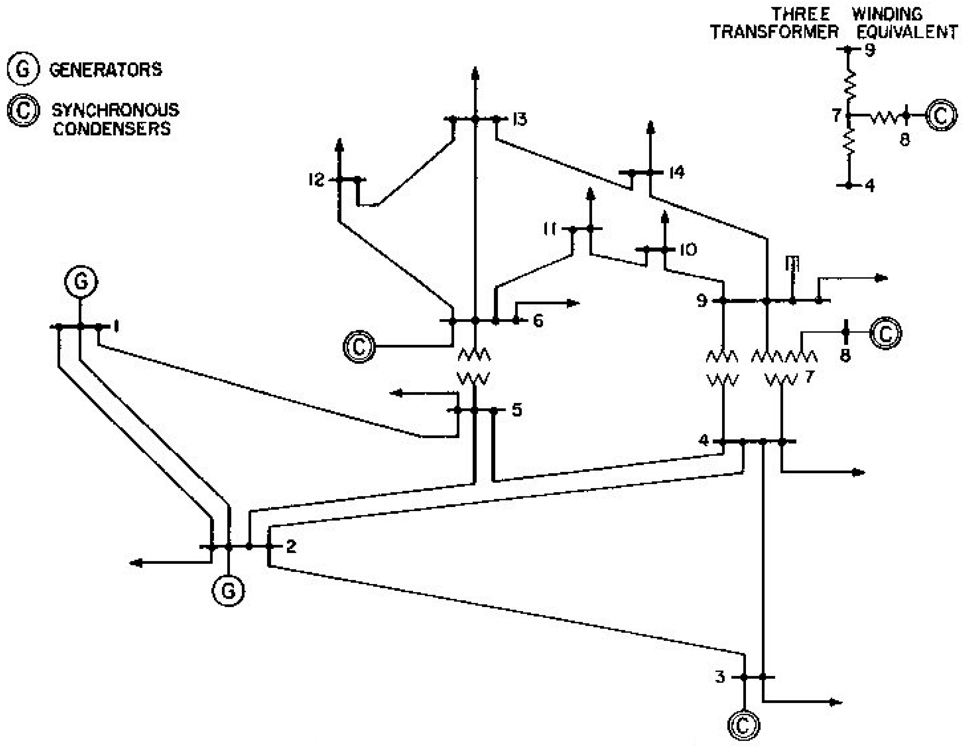
A number of simulations for a specific system have already been performed in order to show how the reliability of the power system has improved. The system used is the IEEE 14-bus Test System [18], which has 20 lines and 14 buses (Figure 3). To compare the outcomes, the system has been tested both with and without the DG associated with some buses. Five contingencies were used in this comparison, after considering 20 contingencies to see how the quantity of contingencies affects the limits of reliability factor. The lines’ data and transformers are shown in [18].

Many publications that explored the resolution of probabilistic power flow and analyzed the reliability of the power network [8,19] have employed this system. The data of the probabilistic loads are from [19].

The power base is 100 MVA and the voltage is 0.95 p.u. and 1.05 p.u. for lower limit and upper limit, respectively, in every bus of the system, excluding the PV buses.

The locations of the generators and the buses are shown in

Table 1. Power generation per group, number of generators per power plant and failure rate.

Bus	Failure Rate	Group Number	Power per Group (MW)
1	0.08	10	50
2	0.09	2	20

. Additionally, each group’s power generation, the quantity of generators for every power plant, and the rate of failure are given.

The contingencies analyzed (in the instance of five contingencies), the line that causes each contingency, and the statistical characteristics of each line are presented in

Table 2. Contingencies considered and number of lines involved in each contingency.

Nº Contingency	Number of Lines Involved	Lines Per Contingency 1
1	1	2
2	1	3
3	1	4
4	1	7
5	1	9

¹ This column shows the number of the line or lines that are involved in a contingency. This denomination refers to column 1 of Table 3.

and

Table 3. Statistical parameters of lines/transformers of IEEE-14 system.

Line Number	Bus From-to	Transmission Capability Limit (p.u.)	Number of Elements	Repair Rate, μ, (years−1)			Failure Rate, λ, (years−1)
1	1–2	3.3	3	650	500	600	0.5	1	0.5
2	1–5	2.0	3	650	800	500	0.8	1.2	0.5
3	2–3	1.0	3	650	500	600	0.5	1	0.5
4	2–4	2.2	3	650	500	600	0.5	1	0.5
5	2–5	0.5	3	300	650	570	0.5	0.5	1
6	3–4	0.5	3	70	400	600	1.2	0.7	0.9
7	4–5	1.0	3	650	500	600	0.5	1	0.5
8	4–7	1.0	3	400	600	500	0.5	0.6	1
9	4–9	1.0	3	650	500	600	0.5	1	0.5
10	5–6	1.0	3	450	450	450	1	1	1
11	6–11	0.15	3	600	600	600	0.5	0.5	0.5
12	6–12	0.15	3	650	550	600	0.9	0.7	0.8
13	6–13	0.3	3	760	700	720	1.4	1	1.2
14	7–8	2.1	3	400	600	500	0.3	0.5	0.4
15	7–9	0.5	3	500	500	500	1	1	1
16	9–10	0.1	3	650	550	550	0.8	0.6	0.6
17	9–14	0.2	3	650	800	500	0.8	1.2	0.5
18	10–11	0.1	3	620	500	400	0.6	0.6	0.6
19	12–13	0.9	3	80	600	800	2	1	0.5
20	13–14	1.0	3	520	300	480	0.8	1	1.1

to estimate the likelihood that every contingency might occur. The lines’ specifications are based on IEEE [20] criteria. In the case study of 20 contingencies, one event is taken into consideration for each line. The maximum transmission capacity for each line is also shown in Table 3.

5.2. Results

Table 4. Probability of happening for the contingency.

Contingency	Probability (%)
Normal	88.5322
1	0.3307
2	0.3193
3	0.3193
4	0.3193
5	0.3193

shows the probability of occurrence for the contingency when five contingencies are simulated. The chance that an event will happen in the normal state (all the lines operate properly) is quite high, which means that the system presents a good reliability.

Generators are connected to improve the system reliability, as shown in

Table 5. System-connected generators.

Bus	Power (p.u.)	Standard Dev.	Voltage (p.u.)
11	0.03	0.00006	1.0435
12	0.06	0.00009	1.0506
13	0.13	0.00013	1.0427

. This table indicates the average power of the generators and their standard deviation. Additionally, the rated voltage for each bus with DG is expressed, since this bus becomes type PV.

As can be seen as an example in Figure 4, the probability improved the load flow through the lines so it complies with the transmission capability limit. Furthermore, Figure 4 depicts the CDFs of power flow through lines 4–5 with and without DG when contingency 3 occurs. The probability that the power flow is below the limit is measured by the CDFs. It can be seen that this probability moves from 0.6274 to 0.8471, which represents an improvement for the system reliability.

Figure 5 shows another example. In this case, the probability improved the voltage compliance with the specified limits. Additionally, this figure depicts the CDFs of voltage of bus 7 with and without DG under anormal state.

It is noted that, as shown in Equation (17), it is necessary to measure F (1.05) and F (0.95). In this case, the value of F (0.95) is zero for the system without DG and with DG. Therefore, the probability of normal voltage is equal to F (1.05). It can be visualized that this probability moves from 0.1730 to 0.6443, which represents an improvement for the system reliability.

Table 6. Reliability index.

(%)	5 Contingencies	20 Contingencies
Without DG	90.1400–100.0000	99.1226–99.7411
With DG	46.4107–59.2707	47.5172–48.1358

shows the values for the reliability index of system (failure probability). Various situations are considered: when five contingencies occur without DG and with DG, and when 20 contingencies occur without DG and with DG.

This table shows that the reliability index improves when DG is connected. Furthermore, the range of values for the reliability index reduces when the number of simulated contingencies increases.

6. Conclusions

In this article, biomass generators have been used to implement a methodology to increase the reliability index of an electrical energy system. The general probability of system outage determines the reliability of the system. Since the reliability of a system cannot be determined accurately, in this work the values of the interval in which this reliability index is contained have been determined.

As the limit values of the reliability interval depend on the number of simulated contingencies, these limits have been calculated assuming that a group of contingencies maintain the system in a normal state (lower limit) and another group of contingencies lead the system to a failure (higher limit).

To determine the reliability indicator, the probabilistic power flow tool has been used. In this work, the probabilistic load flow has been solved by means of the cumulant analytical method, characterizing the random output variables by means of the Gram–Charlier expansion.

The entry data to the issue must be random variables, in order to solve the probabilistic load flow. For this reason, the distributed generation and the loads of the buses have been represented as random variables with a normal distribution. Power plants are represented by means of discrete random variables: Bernoulli distribution if it is a single generator or binomial distribution if it is a plant with several generators. The generators considered as distributed generation are gas engines coupled to alternators. These engines are powered by gasified biomass from olive groves, which are very abundant in Spain.

The results have shown that the reliability index improves when distributed generation is connected. In addition, the interval containing the reliability index is reduced when the number of simulated contingencies increases.

On the other hand, it would be necessary to simulate all possible contingencies to accurately determine the reliability index of the system. This is inappropriate given the high number of combinations of contingencies that can occur, which would lead to a very high computational cost. Thus, the interval where this index is contained can be accepted as a valid result.

As future lines of research, it can be proposed to include generation that is not capable of controlling the voltage of the bus to which it is connected, as can happen with small photovoltaic and wind generators, in order to take into account this type of generators and their associated uncertainties. A mix of different types of generators can also be included, with and without voltage control, and an optimization method can be used to, for example, place these generators correctly within the system and with a suitable size. The objective function of improving system reliability can be combined with other factors, for example, minimizing system losses, minimizing generation costs, etc.

Unbalances have not been considered in this study. A possible way to study this would be to apply this methodology to three-phase electrical systems including single-phase generators.

References

- Borkowska, B. Probabilistic load flow. IEEE Trans. Power Appar. Syst. 1974, 3, 752–759. [Google Scholar] [CrossRef]
- Rubinstein, R.Y. Simulation and the Monte Carlo Method; John Wiley and Sons: New York, NY, USA, 1989. [Google Scholar]
- Li, W. Probabilistic Transmission System Planning; John Wiley and Sons: Hoboken, NJ, USA, 2011. [Google Scholar]
- Anders, G.J. Probability Concepts in Electric Power Systems; John Wiley and Sons: New York, NY, USA, 1990. [Google Scholar]
- Sanabria, I.A.; Dillon, T.S. Stochastic power flow using cumulants and Von Mises functions. Int. J. Electr. Power Energy Syst. 1986, 8, 47–60. [Google Scholar] [CrossRef]
- Zhang, P.; Lee, S.T. Probabilistic load flow computation using the method of combined cumulants and Gram-Charlier expansion. IEEE Trans. Power Syst. 2004, 19, 676–682. [Google Scholar] [CrossRef]
- Morales, J.M.; Pérez-Ruiz, J. Point estimate schemes to solve the probabilistic power flow. IEEE Trans. Power Syst. 2007, 22, 1594–1601. [Google Scholar] [CrossRef]
- Sanabria, L.A.; Dillon, T.S. Power system reliability assessment suitable for a deregulated system via the method of cumulants. Int. J. Electr. Power Energy Syst. 1998, 20, 203–211. [Google Scholar] [CrossRef]
- Meliopoulos, A.P.; Bakirtzis, A.G.; Kovacs, R. Power system reliability evaluation using sto-chastic load flow. IEEE Trans. Power Appar. Syst. 1984, 5, 1084–1091. [Google Scholar] [CrossRef]
- Ruiz-Rodriguez, F.J.; Gomez-Gonzalez, M.; Jurado, F. Optimization of radial systems with biomass fueled gas engine from a metaheuristic and probabilistic point of view. Energy Convers. Manag. 2013, 65, 343–350. [Google Scholar] [CrossRef]
- Gomez-Expósito, A.; Conejo, A.J.; Cañizares, C. Electric Energy Systems, Analysis and Operation; Tailor & Francis Group: Abingdon, UK, 2009. [Google Scholar]
- Canavos, G.C. Probabilidad y estadística. Aplicaciones y métodos; McGraw-Hill: Richmond, VA, USA, 1988. (In Spanish) [Google Scholar]
- Kendall, M.G.; Stuart, A. The Advanced Theory of Statistics, 4th ed.; Macmillan: New York, NY, USA, 1977. [Google Scholar]
- Ruiz-Rodriguez, F.J.; Hernandez, J.C.; Jurado, F. Probabilistic load flow for photovoltaic dis-tributed generation using the Cornish-Fisher expansion. Electr. Power Syst. Res. 2012, 89, 129–138. [Google Scholar] [CrossRef]
- Jurado, F.; Ortega, M.; Cano, A.; Carpio, J. Neuro-fuzzy controller for gas turbine in bio-mass-based electric power plant. Electr. Power Syst. Res. 2002, 60, 123–135. [Google Scholar] [CrossRef]
- Lopez, P.R.; González, M.G.; Reyes, N.R.; Jurado, F. Optimization of biomass fuelled systems for distributed power generation using particle swarm optimization. Electr. Power Syst. Res. 2008, 78, 1448–1455. [Google Scholar] [CrossRef]
- Lopez, P.R.; Jurado, F.; Reyes, N.R.; Galan, S.G.; Gomez, M. Particle swarm optimization for biomass-fuelled systems with technical constraints. Eng. Appl. Artif. Intell. 2008, 21, 1389–1396. [Google Scholar] [CrossRef]
- Power Systems Test Case Archive. Available online: http://www.ee.washington.edu/research/pstca (accessed on 1 July 2022).
- Allan, R.N.; Al-Shakarchi, M.R.G. Probabilistic techniques in a.c. load flow analysis. Proc. IEEE 1977, 124, 154–160. [Google Scholar] [CrossRef]
- IEEE Std 493; IEEE Recommended Practice for the Design of Reliable Industrial and Commercial Power Systems. IEEE: Piscataway, NJ, USA, 2007.
Figure 1.
Line of transmission with a series-connected component.
Figure 2.
Representation of the accumulative distribution function for the voltage in a non-specific bus i.
Figure 3.
IEEE 14-bus Test System Schematic.
Figure 4.
Power flow through lines 4–5 when contingency 3 occurs.
Figure 5.
CDFs of voltage of bus 7 under normal state.