Article

Numerical Study on Peak Shaving Performance of Combined Heat and Power Unit Assisted by Heating Storage in Long-Distance Pipelines Scheduled by Particle Swarm Optimization Method

1
Heating Research Center, Huadian Electric Power Research Institute, 2 Xiyuan Nine Road, Hangzhou 310030, China
2
College of Energy Engineering, Zhejiang University, 38 Zheda Road, Hangzhou 310007, China
*
Author to whom correspondence should be addressed.
Energies 2024, 17(2), 492; https://doi.org/10.3390/en17020492
Submission received: 5 December 2023 / Revised: 6 January 2024 / Accepted: 15 January 2024 / Published: 19 January 2024

Abstract

:
Thermal energy storage in long-distance heating supply pipelines can improve the peak shaving and frequency regulation capabilities of combined heat and power (CHP) units participating in the power grid. In this study, a one-dimensional numerical model was established to predict the thermal lag in long-distance pipelines at different scale levels. The dynamic response of the temperature at the end of the heating pipeline was considered. For the one-way pipe lengths of 10 km, 15 km and 20 km, the response times of the temperature at the distal end were 2.33 h, 2.94 h and 3.54 h, respectively. The longer the flow period, the further the warming-up time is delayed. An optimization scheduling approach was also created to illustrate the peak shaving capabilities of a CHP unit combined with a long-distance pipeline thermal energy storage component. It was demonstrated that the maximum heating load of the unit increased up to 503.08 MW, and the heating load could be expanded in the range of 17.88 MW to 203.76 MW at the minimum electric load of the unit of 104.08 MW. Finally, the particle swarm optimization method was adopted to guide the operating strategy through a whole day to meet both the electric power and heating power requirements. For the optimized case, the comprehensive energy utilization efficiency and the exergy efficiency increase to 64.4% and 56.73%. The thermal energy storage applications based on long-distance pipelines were simulated quantitively and proved to be effective in promoting the operational flexibility of the CHP unit.

1. Introduction

With the large-scale integration of renewable energy sources such as wind power and solar power generation into the grid, the time-varying characteristics on the power supply side are sensibly increasing, leading to intense fluctuations on the power supply side [1]. To maintain a stable power load and provide a standby load, it is significant for CHP units to improve the peak shaving capacity by decreasing the power during the peak periods of renewable energy supply and increasing the power during the off-peak periods. However, with their rigid thermal–electric coupling characteristics, CHP units run with insufficient operational flexibility. To meet these restrictions, heat storage technology is employed in CHP systems to enhance the thermal–electric decoupling capability.
Employing thermal storage components could effectively optimize the thermal–electric decoupling performance. A hot water storage tank [2], molten salt heat storage system [3] and comprehensive TES system [4] have been integrated into CHP facilities to enhance the flexibility of their operating capabilities. However, considering the additional devices, the relevant costs are quite high. On the other hand, district heating networks with long-distance pipelines are capable of storing a large amount of thermal energy with little extra investment [5]. Scheduled by an intelligent dispatching system, the thermal–electric decoupling capability of the source network integration system could be enhanced. The flexible operation performance of CHP units would also be promoted, representing an adaptation that meets the development demand of China’s new power system. Olgierd and Ryszard [6,7] studied the heat and water loss phenomena in DHS with a numerical process and proposed the building of additional tanks or the use of heat storage tanks directly to collect temporary excess water. Their research provided an effective method for enhancing the operational capability of DHS in different operating conditions.
The utilization principle of district heating networks with long-distance pipelines for thermal storage is to make full use of the large thermal inertia of the long-distance pipelines: During the electric peak shaving period, more steam is extracted from steam turbines, and the excess heat resources are stored in district heating networks by raising the networks’ average temperature. By contrast, during the electric peaking period, the extraction flow rate decreases, and much more steam is used for electric power generation. The heating capability of CHP units thus decreases. The previous heat storage in the heating network is then scheduled for release, acting as the thermal energy supply resource temporarily. Considering the complex operating process, developing optimized scheduling strategies is quite crucial for the stability and safety of the system’s operation [8,9]. For more details down to the component level, transient simulation needs to be implemented to assess the specific operation capability [10].
For detailed research issues, scholars have begun to conduct operating optimization studies on district heating systems from different perspectives. Wang et al. [11] and Franco et al. [12] demonstrate that establishing a well-sized thermal energy storage system and a correct operational strategy can help to operate a CHP unit in a constant way, increasing the share for the thermal production and increasing the energy efficiency; the first law efficiency increased from 0.74 to 0.84, and the second law efficiency increased from 0.35 to 0.44. Zheng et al. [13] developed a mixed-integer nonlinear programming model for an integrated energy system with CCHP, incorporating storage to solve the multi-objective optimization problem and determine the best combination of technologies for meeting the energy demand under practical constraints. Martínez et al. [14] introduced an application to the assessment and optimal sizing of thermal storage in CCHP plants for detailed system constructions. Iribarren et al. [15] optimized the system and operation design of thermal energy storage systems in micro-cogeneration plants. The calculation results indicated that the optimal size of storage minimizes the overall cost and the generated emissions. Tehrani et al. [4] studied a smart operation strategy to match the production and consumption profiles of a TES facility coupled with a CHP plant; the annual CHP efficiency increases by 1.12%, and the annual fuel consumption rate and CO2 emissions decrease by 2.6%.
Simulation methodology for CHP/TES has also been implemented widely in recent decades. Thermal–hydraulic analysis code relap5 [16] was employed to simulate water hammer characteristics in district heating networks. Valve modeling is quite crucial in the simulation process. The commercial software Apros [17] was utilized to calculate the hydraulic performance under the guidance of a control strategy coded using MATLAB. Kirchhoff’s law was used in centralized heating system hydraulic balance prediction [18], and network flexibility methodology was also evaluated. A novel three-order scheme was developed to preserve the sharp temperature front in coarse mesh in long-pipe district heating networks [19], which would dramatically decrease the calculation quantity for detailed system prediction. Hou et al. [20] employed the Simulink toolkit to simulate the dynamic characteristics of a comprehensive energy supply system. Wang et al. [21] and Zheng et al. [22] reviewed integrated multi-energy-system flexibility options, and energy storage and future ancillary services were investigated.
However, the recent simulation studies were not much related to heat storage capacity and the thermal inertia of heating networks. In order to utilize the heat storage capacity to enhance the heat and power decoupling capability of CHP units, it is necessary to establish a dynamic model of a district heating network. This paper presents a study of the heat storage performance of long-pipe heating networks and an analysis of the peak shaving capacity of a power plant scheduled using the particle swarm optimization method.

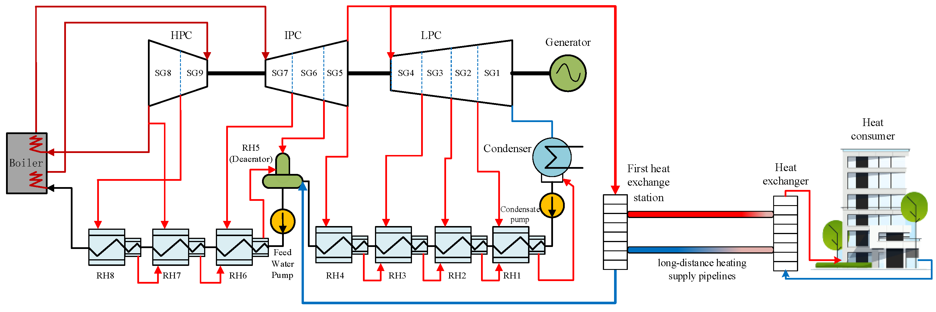
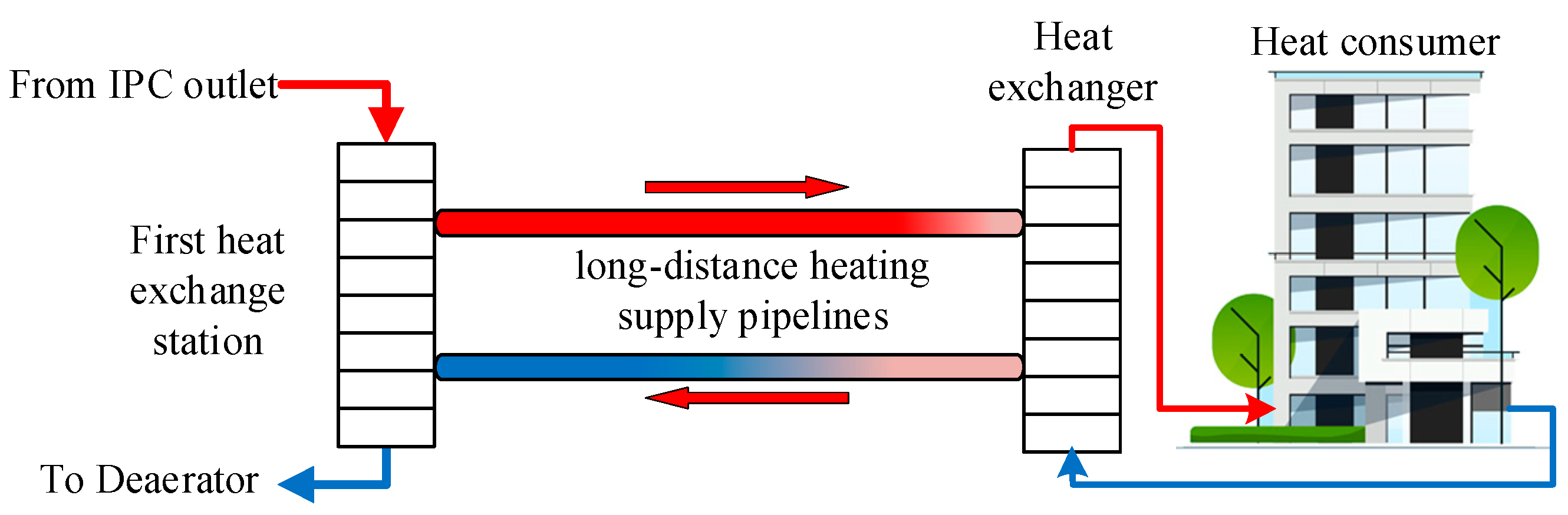
2. Dynamic Simulation Model

In the cogeneration unit, the steam turbine is employed mainly to generate electricity. Steam is partially extracted to heat circulation water of the primary heating network in the primary heating station. The hot circulation water is pumped to the heat exchange station through the heat network pipeline to supply thermal energy to buildings. In winter, the steam extraction capacity is almost fixed, which imposes restrictions on the electric peak shaving flexibility of the cogeneration unit. The thermal energy storage in long-distance heating supply pipelines could improve the peak shaving and frequency regulation capabilities of cogeneration units participating in the power grid. To investigate the inherent characteristics, numerical models were established in this research.
A transient numerical model was developed to simulate thermal performance in the steam turbine and long-distance heating supply pipelines. Considering that the steam travels at supersonic speed through the steam turbine blade, a quasi-steady-state assumption was used in the turbine model establishment.

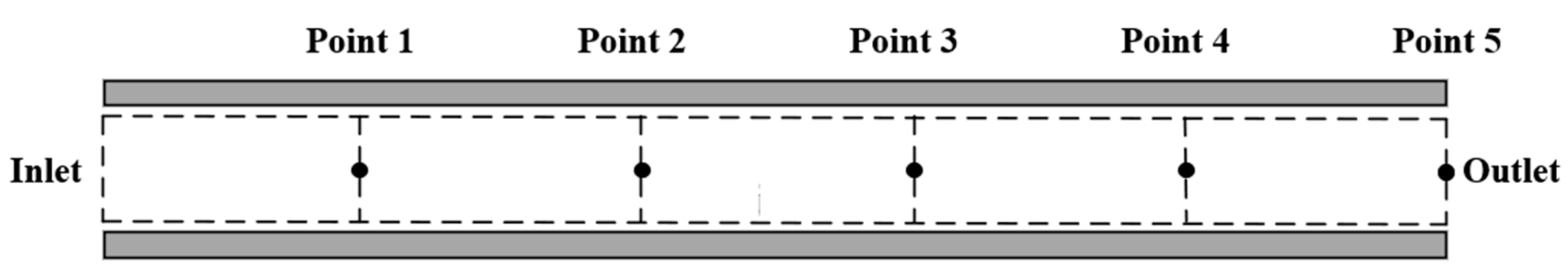
2.1. Heat Transfer Model

When the hot circulation water flows through the pipeline, heat loss occurs due to the large temperature difference between hot water and the ambient atmosphere. In the radial direction, the total thermal resistance is composed of the following serial components:
The thermal resistance from the hot water to the inside pipe wall,
R i n = 1 π α i n D i n
The pipe wall thermal resistance,
R p i p e = 1 2 π λ p i p e ln D o u t , p i p e D i n , p i p e
The thermal insulation material thermal resistance,
R l a y e r = 1 2 π λ l a y e r ln D o u t , l a y e r D o u t , p i p e
The soil thermal resistance,
R s o i l = 1 2 π λ s o i l ln 4 x D o u t , l a y e r
Compared with the other thermal resistances, R i n and R p i p e have a lower order of magnitude and can be neglected. Therefore, the total thermal resistance becomes
R = R l a y e r + R s o i l
In the axial direction, energy conservation equations were discretized to simulate the thermal lag characteristics of long-distance heating supply pipelines. A one-way heating pipeline was divided into 100 nodes equidistantly, and the lumped parameter method was employed for each node. Figure 1 illustrates the discrete scheme of the transient calculation methodology. An explicit scheme for time sequences and a first-order upwind scheme were utilized in the code.
Regarding the water and steam medium as an incompressible fluid, in node i, the explicit form of the energy conservation equation becomes
G h n 0 , inlet G h n 0 , outlet T n 0 T s o i l R n L i 1 + β π D i , o u t , l a y e r = h n t ρ π D i , o u t , l a y e r 2 2 L i
When Equation (6) is discretized with a first-order difference scheme, the differential equation turns into an algebraic equation, which can be solved numerically.
G h n 0 , inlet G h n 0 , outlet T n 0 T s o i l R n L i 1 + β π D i , o u t , l a y e r Δ t = ρ π D i , o u t , l a y e r 2 2 L i h n h n 0

2.2. Pressure Drop Model

Pressure drop was included in the hydraulic model. For a circular pipe, the pressure drop is mainly caused by friction resistance Δ P f r i c ,
Δ P f r i c = 6.88 × 10 3 K 0.25 G n 0 2 L i ρ D n 5.25
And the pressure drop equation for each node can be written as
p i , outlet = p i , inlet Δ P f r i c
The pressure of node i at the n0 time level is
p i , n 0 = p i , outlet + p i , inlet 2

2.3. Model of Turbine

The Flugel formula is the theoretical basis for predicting the variable condition properties of steam turbines in CHP units. The original form is
G 1 G 1 b = p 1 2 p 2 2 p 1 b 2 p 2 b 2 T 1 b T 1
In the formula, letters with b subscript represent parameters in basic working conditions as reference data, and letters without b subscript represent parameters in variable conditions.
Backpressure, a parameter determined by the working condition of the condenser, is a crucial parameter for achieving the maximum work output for the turbine. It is necessary to determine the temperature of condensed water t c o n d to determine the backpressure at the outlet of the low-pressure cylinder of the turbine. The temperature of condensed water is mainly governed by condenser and circulation water parameters, as given in the following formula:
T c o n d = T c i r c , i n l e t + G e x h h e x h h e x h C c i r c G c i r c 1 exp k c o n d F c o n d C c i r c G c i r c

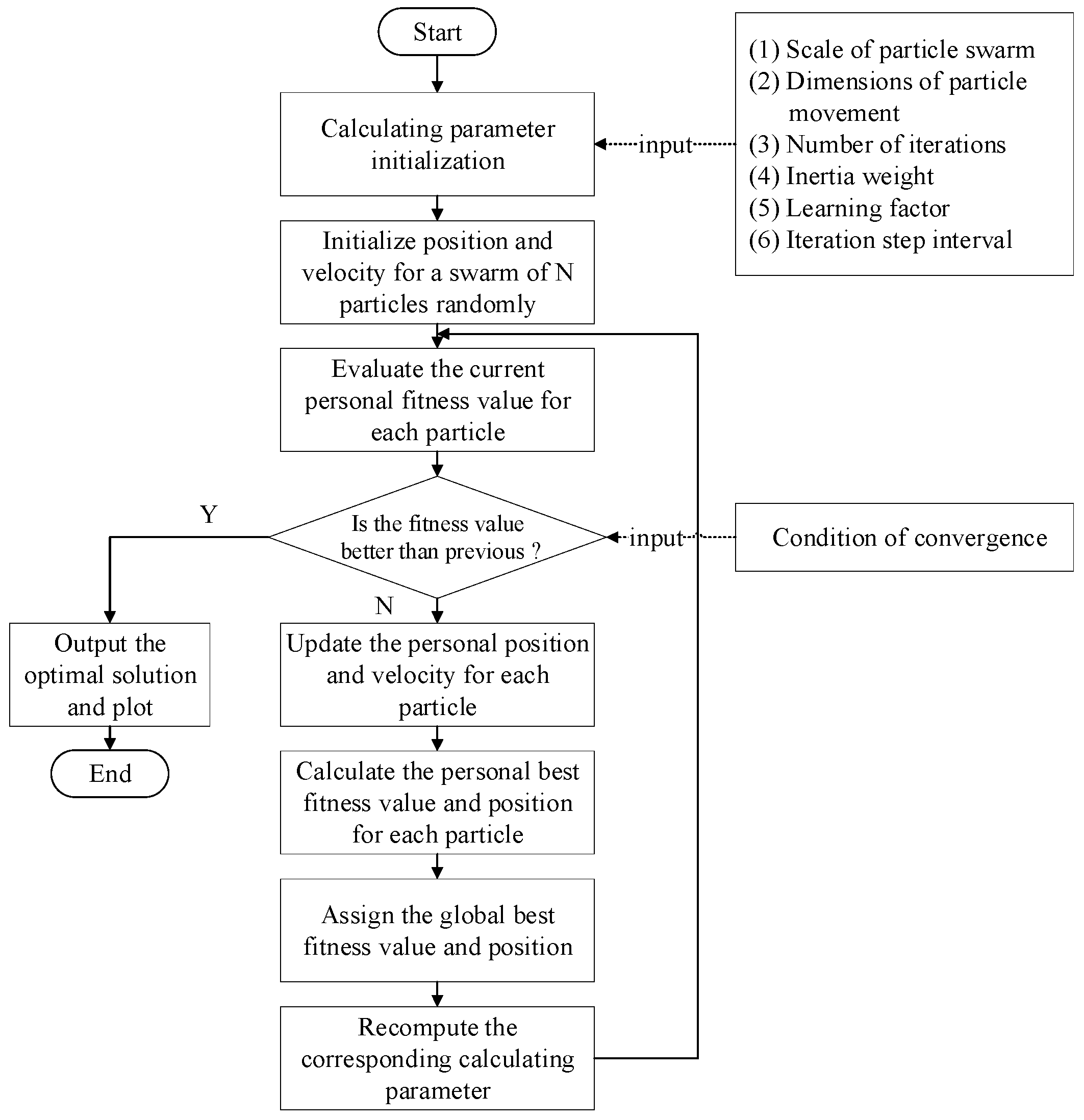
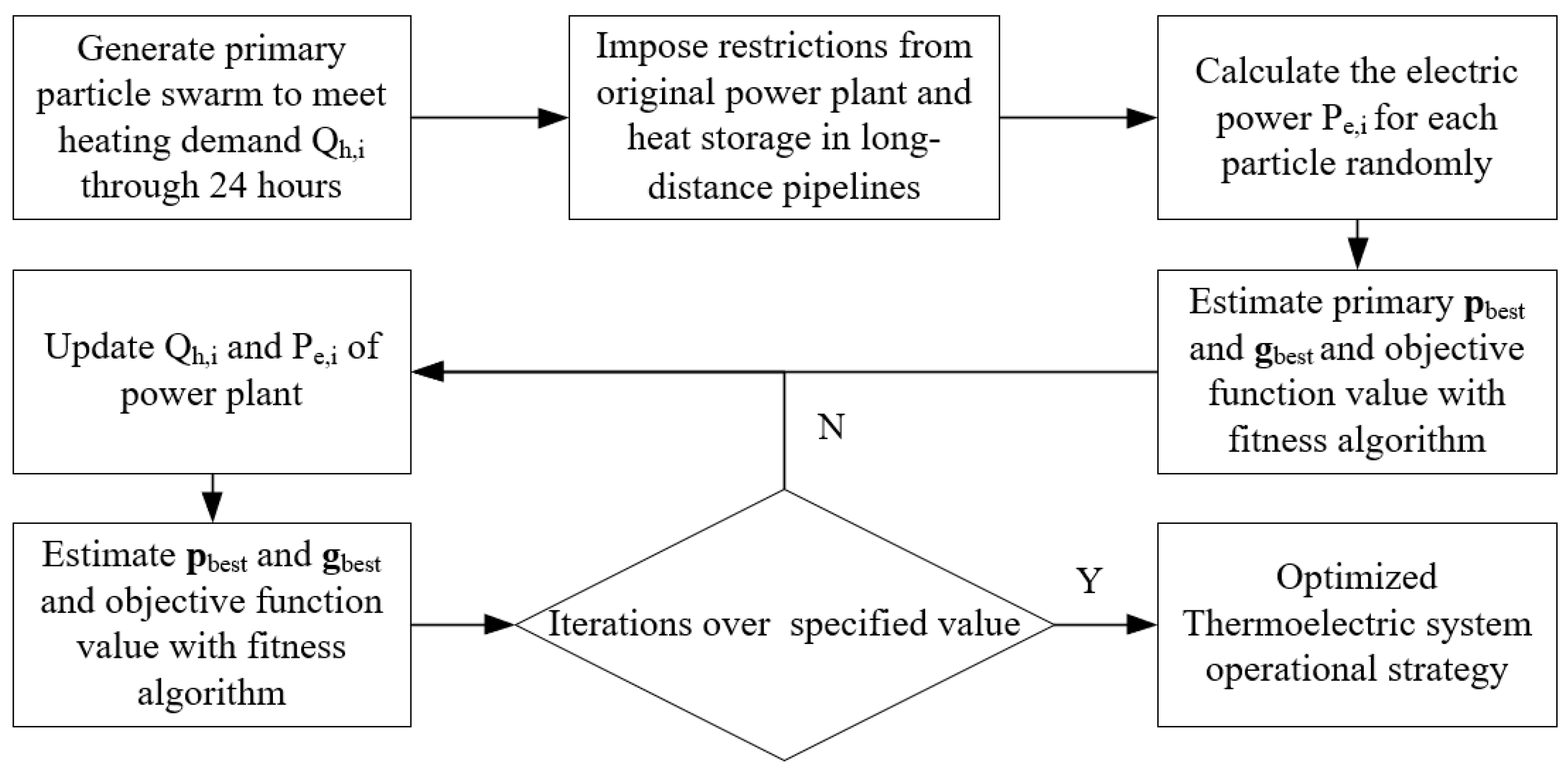
2.4. Particle Swarm Optimization Method

In 1995, particle swarm optimization (PSO) was proposed by Kennedy and Eberhart [23] to imitate the social behavior of animals. The swarm-based stochastic algorithm has been extended for utilization in CHP [24] operation optimization. To receive the optimal solution, the personal best position ( p b e s t , i ) for each particle and the global best position ( g b e s t , i ) in the swarm need to be evaluated. The basic calculation strategy is performed as follows:
p b e s t , i t = x i * f x i * = min k = 1 , 2 , , t f x i k
where i { 1 , 2 , , N } , and
g b e s t t = x * t f x * t = min i = 1 , 2 , , N k = 1 , 2 , , t f x i k
In the formula, i represents each particle’s tag, t denotes the current iteration step, f is employed to describe the objective function to be calculated, x is the particle’s position vector and v is the velocity. N denotes the total number of particles. v and x should be refreshed by the formula as follows at t + 1 iteration:
v i t + 1 = ω v i t + c 1 r 1 p b e s t i t x i t + c 2 r 2 g b e s t t x i t
where ω represents the inertia weight as a balancing factor for local and global exploration equilibrium, r 1 and r 2 are random vectors. c 1 and c 2 are acceleration coefficients. The calculation flowchart is illustrated in Figure 2.

3. Results

3.1. Reference Case

A 330 MW CHP was selected as the reference case to simulate the thermal–electric decoupling techniques. The configuration of the thermodynamic system is charted below in Figure 3. The heat power decoupling technique based on a long-distance pipeline thermal energy storage component was studied for the reference power plant. The main feed water system includes seven shell-and-tube heat exchangers (low-pressure heat exchangers RH1-RH4 and high-pressure heat exchangers RH6-RH8) and a mixing-type heat exchanger (deaerator RH5). The heat sources are all from the extraction of steam from the turbine.
In this 330MW CHP unit, one steam extraction point was set at the outlet of the intermediate pressure cylinder to heat the long-distance heating supply pipelines. In the calculation process, the steam pressure to the regenerative heaters can be calculated with the following formula according to the Flugel formula:
P r = P 5 2 + ( G 1 G 1 b ) 2 ( P r b 2 P 5 b 2 ) ( r = 6   to   8 )
And the extraction steam pressures in LPC can be calculated as follows:
P r = P c 2 + ( G 1 G 1 b ) 2 ( P r b 2 P c b 2 ) ( r = 2   to   5 )
where the r represents the position of the extraction point after the stage group.
Then, a long-distance heating supply pipeline was built with the CHP for heating supply to remote heat consumers. The layouts of the entire system are charted in Figure 4. The one-way pipeline lengths of 10 km, 15 km and 20 km were calculated.

3.2. Performance Characteristics of Long-Distance Pipeline Thermal Energy Storage Component

Calculation oriented to thermal storage characteristics through long-distance heating pipelines was performed with the transient modeling methodology mentioned in Section 2.1 and Section 2.2. Cases with one-way pipeline lengths of 10 km, 15 km and 20 km were built. Temperature fluctuations were focused on. In each case, the pipelines received heat in the first heat exchange station and partially delivered heat to the remote heat exchanger, as shown in Figure 5. The heat storage and supply procedures were performed and analyzed.
The calculation boundary conditions were defined in the analysis code according to the parameters in Table 1. It is worth mentioning that the total thermal power for the heat exchanger remains constant during the calculation. Thus, the difference in temperature between the inlet and outlet of the heat exchanger was set as a constant. The heat storage and supply procedures were simulated in each case: During 0 h–20 h, the first heat exchange station worked for heat storage. During 20 h–24 h, the first heat exchange station was out of service, and the heat supply only depended on the sensible heat. To monitor the spatial distribution and response characteristics of temperature fluctuation along the long-distance pipeline, five monitoring points were installed, as shown in Figure 6, in both the feedwater pipeline and return pipeline.
The calculation results are displayed in Figure 7. Subplots (a), (c) and (e) illustrate temperature distributions along the feedwater pipelines. Temperature waves occurred periodically from point 1 to point 5 in sequence. For the first wave, temperatures rose to 75.23 °C, 74.95 °C and 74.62 °C in the 10 km, 15 km and 20 km cases, respectively. A similar conclusion could also be demonstrated by the data in (b), (d) and (f), the data monitored along the return pipelines. According to the energy conservation relation, the tiny temperature reductions should be mainly caused by the heat loss model embedded in Formula (6) with the linear heat loss coefficient β.
It could be found obviously that the temperature fluctuation response is related to the pipeline distance. For the first wave in each case through the feedwater pipeline and return pipeline, the response time at point 1 in each pipeline in the simulation was calculated and is listed in Table 2. The results demonstrated that the time for warming up at point 1 on each pipeline is positively associated with the flow period or the flow distance from the inlet of the pipelines. The longer the flow period, the further the warming-up time is delayed. The variation should be influenced mainly by Equation (6): for the fluid flow, the heat loss term T n 0 T s o i l R n L i 1 + β π D i , o u t , l a y e r decreases the fluid enthalpy h n 0 , inlet gradually, which governs the slope of the temperature function most on the left side of the formula. As a result, the response time increases with the fluid flow, and the heat loss mechanism should be studied carefully to raise the efficiency of heat utilization and make the temperature change more sensitive.
As shown in Figure 8 and Table 3, the temperature distributions influenced by the initial temperatures in the feedwater pipe were also investigated. Similar conclusions were drawn from the temperature response time results. When the initial temperature is raised, more heat is transferred into the ambient atmosphere due to a large temperature difference, which weakens the slope of the temperature change and finally extends the heat transfer response time. As a result, the heat loss process should be designed carefully, not only to raise the efficiency of heat storage, but also to make the whole process much more flexible.

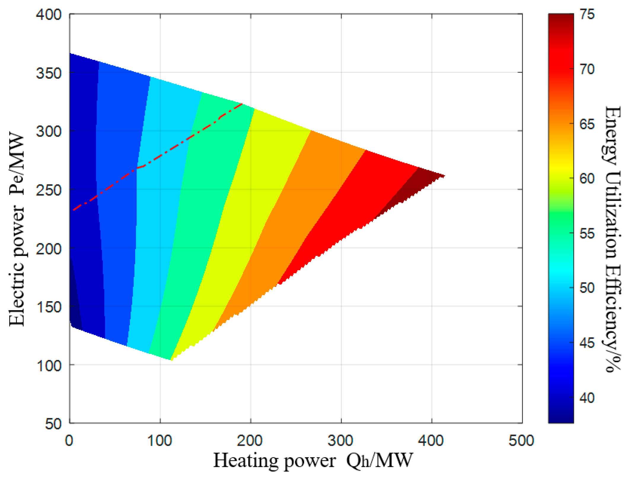
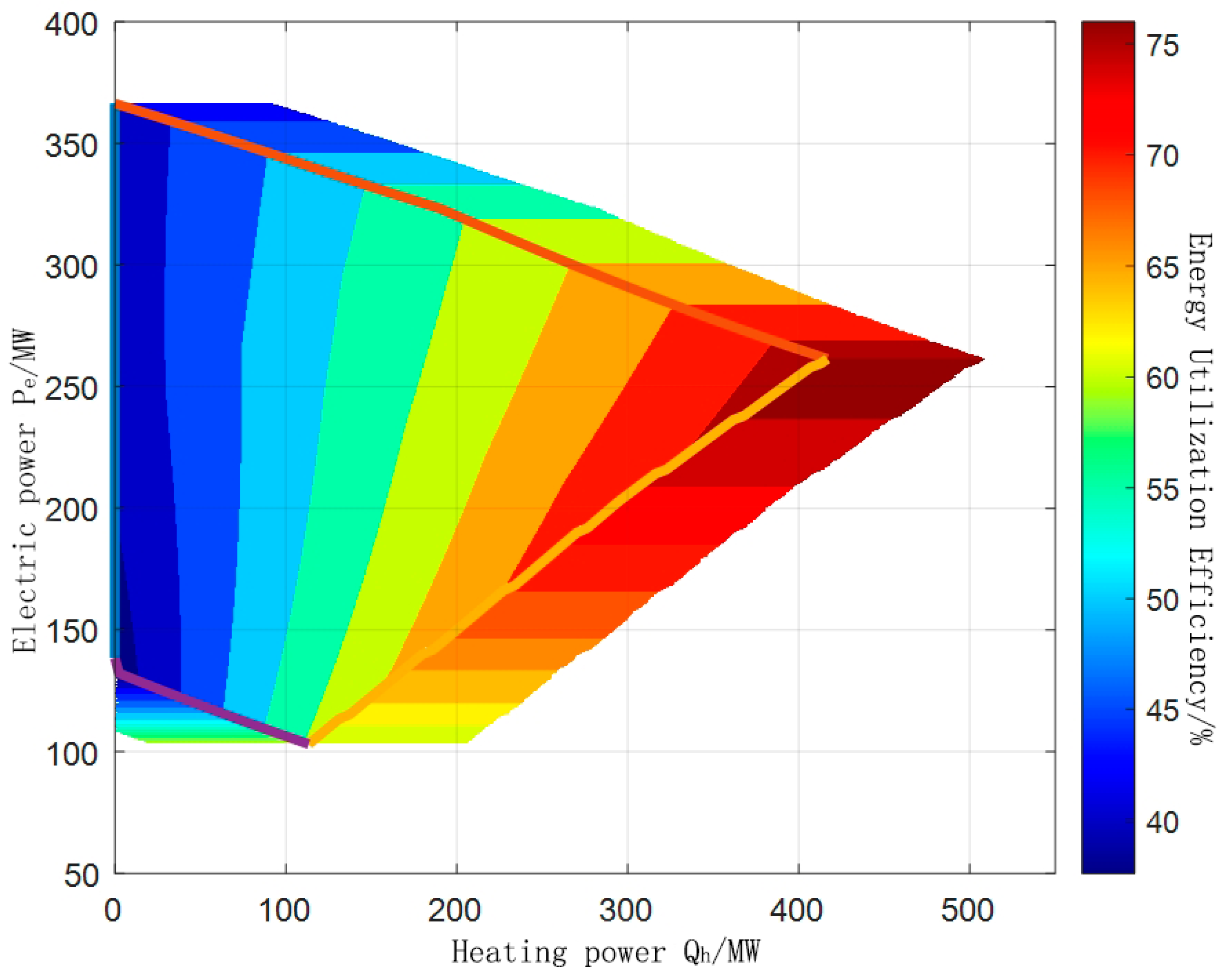
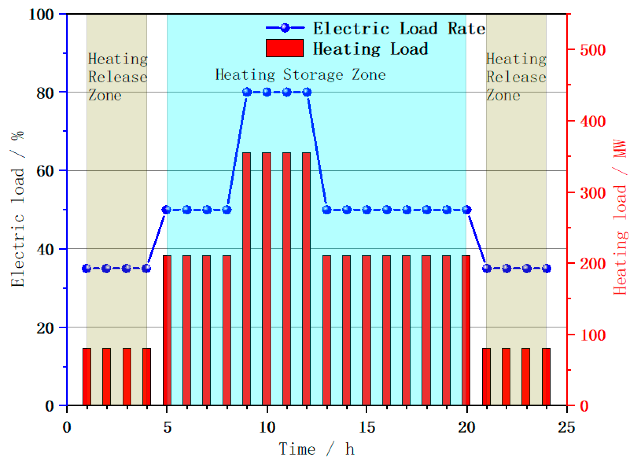
3.3. Peak Shaving Performance Optimization

The swarm optimization method mentioned in Section 2.4 was used to enhance operational flexibility based on the energy storage capability of long-distance heating pipelines. To implement the optimization method, a 330 MW cogeneration unit was selected for heating the heating network. The system diagram of a single unit combined with long-distance heating supply pipelines is shown in Figure 4. According to the thermodynamic property of turbine units of the power plant, the original energy utilization efficiency distribution was calculated and is displayed in Figure 9. The dot–dash line represents the fully open state of the control valve after the steam heating outlet when the thermal power is increased.
The operational domain was restricted by the boundaries described below. The maximum value of the main steam flow acted as the superior limit,
P e = 0.229 Q h + 366.7
for partially opening the control valve (on the left side of the dot–dash line) and
P e = 0.0001803 Q h 2 0.3835 Q h + 389.9
for fully opening the control valve (on the right side of the dot–dash line), where P e and Q h represent the electric power and heating power.
The minimum value of the condensing flow limited the domain on the right.
P e = 0.5289 Q h + 44.76
The minimum value of the main steam flow defined the inferior boundary.
P e = 0.2683 Q h + 132.9
The local energy utilization efficiency was calculated as follows:
η e n , l o c = P e , i + Q h , i B i Q L H V
The local exergy efficiency was calculated as follows:
η e x , l o c = P e , i + ( E s u p p l y , i E r e t u r n , i ) B i Q H H V
The subscript i is used to identify different working conditions. Considering the heating storage capacity based on the long-distance pipelines, a 92.94 MW heating storage and supply capability could be utilized to support the flexible operation requirement. The operational domain is expanded along the heating power direction. The additional heating storage components obviously enhance the thermal–electric decoupling ability of the thermoelectric unit and enlarge the working condition domain with high energy efficiency. When heating power increases to more than 300 MW, the efficiency can mostly reach over 70%. The energy utilization efficiency distribution is charted in Figure 10.
During the heat supply operation of the unit with a heat storage component, the electrical load regulation range stays the same as before. However, the heating supply range is widely expanded. The total heating supply load could reach 503.08 MW temporarily. If the heating load is fixed, the thermoelectric unit will operate on a vertical line in the graph. Compared with the original operating characteristics, when receiving peak shaving instructions, the unit can use thermal energy storage for heat supply, enhancing the unit’s ability to participate in peak shaving and improving the flexibility of unit operation.
The particle swarm optimization method was employed to optimize the operation strategy for 24 h for a power plant combined with a heat storage component. Although the optimization is governed by the thermoelectric characteristics illustrated by Figure 10, a time-delay characteristic is also considered:
t d = π ρ L D i n 2 4 G
In this case, the length of one-way long-distance pipeline is 15 km. The flow rate is 815.0 kg/s. Conservations in electric power supply and heating supply are also defined,
P e , i = P e , j   ( i , j = 1 , 2 , , 24 )
and
i = 1 24 Q h , i = j = 1 24 Q h , j
The subscripts i and j represent the supply-side parameter and demand-side parameter, respectively. The optimization calculation process is illustrated in Figure 11.
To accelerate the iteration process, a penalty function was utilized in the fitness algorithm, as shown in Figure 12. An extremely large number was attached to the objective function to penalize infeasible particles. The penalty function could eliminate the out-of-date particles gradually and accelerate the convergence of the particle swarm to the optimized result.
Based on the optimization methodology, several working scheduling strategies were compared to meet a daily specific electric and heating requirement. The oriented electric load tendency is a daily tendency for the 330 MW power plant, including a simple peak and valley, as shown by the blue curve in Figure 13. The heating load is fixed to 190 MW.
To evaluate the scheduling strategy, the comprehensive energy utilization efficiency and exergy utilization efficiency were calculated in each case. The comprehensive energy utilization efficiency was estimated by taking the average value of local energy utilization efficiency defined in Formula (22):
η e n , c o m p = η ¯ e n , l o c = 1 24 i = 1 24 P e , i + Q h , i B i Q L H V
And exergy efficiency was calculated as follows:
η e x , c o m p = η ¯ e x , l o c = 1 24 i = 1 24 P e , i + ( E s u p p l y , i E r e t u r n , i ) B i Q H H V
For the first scheduling strategy, the local energy utilization efficiency of the power plant was required for the electric load peak. During 9 h–12 h, the heating load of the power plant increases to 405 MW, and the local energy utilization efficiency and exergy efficiency can reach 76.71% and 58.55%. And in the heating release zone, the heating load is supplied by the storage heat and planned extraction of steam heat. The comprehensive energy utilization efficiency and exergy efficiency for the daily scheduling strategy reach 63.65% and 56.67%. The operation strategy is illustrated in Figure 13.
For the second scheduling strategy, a balanced policy is trialed. Here, 355.09 MW and 210.36 MW heating loads are implemented in the heating storage zone for the peaking part and ordinary part. For the peaking period, the energy utilization efficiency and exergy efficiency are 73.23% and 58.5%, respectively, much higher than the values during the ordinary period (68.23% and 57.16%). The comprehensive energy utilization efficiency and exergy efficiency for the second scheduling strategy reach 64.05% and 56.7%, which are better than the local optimal case values; the scheduling strategy is charted in Figure 14.
Finally, the particle swarm optimization method was adopted for the scheduling. Here, 305.18 MW and 227.1 MW heating loads were extracted from the power plant into the heating pipeline. The operation strategy is shown in Figure 15. During the peaking period, the energy utilization efficiency was 69.63%, a little bit lower than the value during the ordinary period (70.14%). For the exergy efficiency, the value during the peak period could reach 58.45%, larger than that during the ordinary period (57.24%). However, the comprehensive energy utilization efficiency and exergy efficiency were both optimized, reaching the peak values of 64.40% and 56.73%. The comparison results are listed and compared in Table 4.

4. Conclusions

In this study, a method of thermal–electric decoupling based on heating storage in long-distance pipelines was studied with a simulation process. A one-dimensional numerical model was established to predict the thermal lag in long-distance pipelines. The particle swarm optimization method was also employed to optimize the working scheduling strategy for the daily operation of the thermal–electric decoupling system, and the results are as follows:
The dynamic response of the temperature at the end of the heating pipeline was considered. The longer the flow period, the further the warming-up time is delayed. For the one-way pipe lengths of 10 km, 15 km and 20 km, the response times of the temperature at the distal end were 2.33 h, 2.94 h and 3.54 h, respectively.
The PSO method was also adopted to guide the operating strategy through a whole day to meet both electric power and heating power requirements. By enhancing the electric–thermal decoupling performance relying on the CHP unit combined with long-distance pipeline thermal energy storage component, it was demonstrated that the maximum heating load of the unit increased to 503.08 MW, and the heating load could be expanded in the range from 17.88 MW to 203.76 MW at the minimum electric load of the unit, 104.08 MW. For the optimized case, the comprehensive energy utilization efficiency and the exergy efficiency increase to 64.4% and 56.73%.
The thermal–hydraulic simulation and schedule optimization process for a thermal–electric decoupling system based on thermal energy storage applications through long-distance pipelines presented in this paper provide a structure for quantitively estimating working performance. With this preliminary toolkit, practical models such as the overall heat losses associated with the use of long-distance heat supply pipelines for thermal energy storage could be studied to indicate more operational characteristics of decoupling systems in future research.

Author Contributions

Conceptualization, H.J. and L.Z.; methodology, H.J.; software, H.J.; investigation, Y.W.; data curation, Y.F.; writing, H.J.; supervision, L.Z. All authors have read and agreed to the published version of the manuscript.

Funding

This research received no external funding.

Data Availability Statement

Data are contained within the article.

Conflicts of Interest

Authors Haoran Ju, Yongxue Wang, Yiwu Feng and Lijun Zheng were employed by the Huadian Electric Power Research Institute. The remaining authors declare that the research was conducted in the absence of any commercial or financial relationships that could be construed as a potential conflict of interest.

Nomenclature

SymbolDescriptionUnit
B coal consumption ratekg/s
c acceleration coefficients-
C specific heat capacityJ/(kg °C)
D diameterm
E exergyJ
F heat exchange aream2
f objective function-
G heating water flow ratekg/s
h enthalpykJ/kg
k heat transfer coefficientW/(m2 °C)
L lengthm
N total number of particles-
P pressurePa
Δ P pressure lossPa
P e electric powerMW
Q h heating powerMW
Q L H V lower heating valueMJ/kg
R thermal resistancem2 °C/W
T temperature°C
t times
Δ t time steps
x burial depth of the heating pipelinem
Matrix
g global particle position
p personal particle position
r random vector
v particle velocity
x particle position
Greek Symbols
α heat release coefficient W/(m2 °C)
β local heat loss coefficient%
ρ density of fluidkg/m3
λ thermal conductivityW/(m °C)
K equivalent absolute roughness of wallm
ω inertia weight
Subscripts and superscripts
1 before stage group
2 after stage group
b basic working condition
b e s t best particle
c i r c circulation water
c o m p comprehensive
c o n d condenser
d time delay
e n energy utilization
e x exergy
e x h exhaust steam flow
f r i c friction
i the i node or the i particle
i n inner wall
i n l e t inlet of a node
l a y e r outer wall of insulation layer
l o c local
n the n time level
n 0 current time level
o u t outer wall
o u t l e t outlet of a node
p i p e heating pipeline
r e t u r n return water in heating pipeline
s o i l soil
s u p p l y supply water in heating pipeline
Abbreviations
CCHPcombined cooling, heating and power
CHPcombined heat and power
HHVhigh heat value
LHVlow heat value
PSOparticle swarm optimization
TESthermal energy storage

References

  1. Liu, S.; Shen, J. Modeling of Large-Scale Thermal Power Plants for Performance Prediction in Deep Peak Shaving. Energies 2022, 15, 3171. [Google Scholar] [CrossRef]
  2. Li, Y.; Sun, F.; Zhang, Q.; Chen, X.; Yuan, W. Numerical Simulation Study on Structure Optimization and Performance Improvement of Hot Water Storage Tank in CHP System. Energies 2020, 13, 4734. [Google Scholar] [CrossRef]
  3. Wang, B.; Ma, H.; Ren, S.; Si, F. Effects of integration mode of the molten salt heat storage system and its hot storage temperature on the flexibility of a subcritical coal-fired power plant. J. Energy Storage 2023, 58, 106410. [Google Scholar] [CrossRef]
  4. Mostafavi Tehrani, S.S.; Saffar-Avval, M.; Behboodi Kalhori, S.; Mansoori, Z.; Sharif, M. Hourly energy analysis and feasibility study of employing a thermocline TES system for an integrated CHP and DH network. Energy Convers. Manag. 2013, 68, 281–292. [Google Scholar] [CrossRef]
  5. Brown, A.; Foley, A.; Laverty, D.; McLoone, S.; Keatley, P. Heating and cooling networks: A comprehensive review of modelling approaches to map future directions. Energy 2022, 261, 125060. [Google Scholar] [CrossRef]
  6. Ryszard, Z.; Niemyjski, O. Influence of Different Operating Conditions of a District Heating and Cooling System on Heat Transportation Losses of a District Heating Network. IOP Conf. Ser. Mater. Sci. Eng. 2019, 471, 042019. [Google Scholar]
  7. Niemyjski, O.; Zwierzchowski, R. Impact of Water Temperature Changes on Water Loss Monitoring in Large District Heating Systems. Energies 2021, 14, 2060. [Google Scholar] [CrossRef]
  8. Liu, M.; Ma, G.; Wang, S.; Wang, Y.; Yan, J. Thermo-economic comparison of heat–power decoupling technologies for combined heat and power plants when participating in a power-balancing service in an energy hub. Renew. Sust. Energy Rev. 2021, 152, 111715. [Google Scholar] [CrossRef]
  9. Liu, M.; Liu, M.; Chen, W.; Yan, J. Operational flexibility and operation optimization of CHP units supplying electricity and two-pressure steam. Energy 2023, 263, 125988. [Google Scholar] [CrossRef]
  10. Ye, L.; Yu, H.; Wang, M.; Wang, Q.; Tian, W.; Qiu, S.; Su, G.H. CFD/RELAP5 coupling analysis of the ISP No. 43 boron dilution experiment. Nucl. Eng. Technol. 2022, 54, 97–109. [Google Scholar] [CrossRef]
  11. Wang, J.; Jing, Y.; Zhang, C. Optimization of capacity and operation for CCHP system by genetic algorithm. Appl. Energy 2010, 87, 1325–1335. [Google Scholar] [CrossRef]
  12. Franco, A.; Versace, M. Multi-objective optimization for the maximization of the operating share of cogeneration system in District Heating Network. Energy Convers. Manag. 2017, 139, 33–44. [Google Scholar] [CrossRef]
  13. Zheng, X.; Wu, G.; Qiu, Y.; Zhan, X.; Shah, N.; Li, N.; Zhao, Y. A MINLP multi-objective optimization model for operational planning of a case study CCHP system in urban China. Appl. Energy 2018, 210, 1126–1140. [Google Scholar] [CrossRef]
  14. Martínez-Lera, S.; Ballester, J.; Martínez-Lera, J. Analysis and sizing of thermal energy storage in combined heating, cooling and power plants for buildings. Appl. Energy 2013, 106, 127–142. [Google Scholar] [CrossRef]
  15. Pérez-Iribarren, E.; González-Pino, I.; Azkorra-Larrinaga, Z.; Gómez-Arriarán, I. Optimal design and operation of thermal energy storage systems in micro-cogeneration plants. Appl. Energy 2020, 265, 114769. [Google Scholar] [CrossRef]
  16. Kaliatka, A.; Vaišnoras, M.; Valinčius, M.; Kaliatka, T. RELAP5 application for water hammer analysis in different thermal-hydraulic systems. Int. J. Thermofluids 2022, 14, 100154. [Google Scholar] [CrossRef]
  17. Bastida, H.; Oo, C.E.U.; Abyesekera, M.; Qadrdan, M. Modelling and control of district heating networks with reduced pump utilisation. IET Energy Syst. Integr. 2021, 3, 13–25. [Google Scholar] [CrossRef]
  18. Zhong, W.; Chen, J.; Zhou, Y.; Li, Z.; Lin, X. Network flexibility study of urban centralized heating system: Concept, modeling and evaluation. Energy 2019, 177, 334–346. [Google Scholar] [CrossRef]
  19. Wang, H.; Meng, H. Improved thermal transient modeling with new 3-order numerical solution for a district heating network with consideration of the pipe wall’s thermal inertia. Energy 2018, 160, 171–183. [Google Scholar] [CrossRef]
  20. Hou, Y.; Chen, P.; Jin, Y.; Zhang, C.; Li, W.; Gao, C.; Xiang, Y. Performance analysis of a small lead-cooled fast reactor coupled with a copper-chloride cycle hydrogen production system. Int. J. Hydrogen Energy 2024, 49, 1538–1549. [Google Scholar] [CrossRef]
  21. Wang, J.; Zong, Y.; You, S.; Træholt, C. A review of Danish integrated multi-energy system flexibility options for high wind power penetration. Clean Energy 2017, 1, 23–35. [Google Scholar] [CrossRef]
  22. Zheng, W.; Lu, H.; Zhang, M.; Wu, Q.; Hou, Y.; Zhu, J. Distributed Energy Management of Multi-Entity Integrated Electricity and Heat Systems: A Review of Architectures, Optimization Algorithms, and Prospects. IEEE Trans. Smart Grid 2023, 1. [Google Scholar] [CrossRef]
  23. Eberhart, R.; Kennedy, J. A New Optimizer using particle swarm theory. In Proceedings of the MHS’95. Proceedings of the Sixth International Symposium on Micro Machine and Human Science, Nagoya, Japan, 4–6 October 1995; pp. 39–43. [Google Scholar]
  24. Wang, Z.; Gu, Y.; Zhao, Z.; Lu, S. Operational optimization on large-scale combined heat and power units with low-pressure cylinder near-zero output. Energy Sci. Eng. 2023, 11, 2081–2095. [Google Scholar] [CrossRef]
Figure 1. Numerical scheme of transient calculation methodology through the pipeline.
Energies 17 00492 g001
Figure 2. Flowchart of particle swarm optimization algorithm.
Energies 17 00492 g002
Figure 3. The original configuration of 330 MW CHP.
Energies 17 00492 g003
Figure 4. CHP with heat storage system based on long-distance heating supply pipelines.
Energies 17 00492 g004
Figure 5. Heat storage facility based on long-distance heating supply pipelines.
Energies 17 00492 g005
Figure 6. Monitoring point distribution.
Energies 17 00492 g006
Figure 7. Temperature distributions and responses in pipes with different distances. Subfigures (a,c,e) illustrate temperature distributions along feedwater pipelines in 10 km, 15 km and 20 km cases. Subfigures (b,d,f) display the data monitored along return pipelines in 10 km, 15 km and 20 km cases.
Energies 17 00492 g007
Figure 8. Temperature distributions in pipes with different initial temperatures of feedwater. Subfigures (a,c,e) illustrate temperature distributions along feedwater pipelines in 10 km, 15 km and 20 km cases. Subfigures (b,d,f) display the data monitored along return pipelines in 10 km, 15 km and 20 km cases.
Energies 17 00492 g008
Figure 9. The original energy utilization efficiency distribution. The dot–dash line indicates a fully opened control valve of the turbine.
Energies 17 00492 g009
Figure 10. The energy utilization efficiency distribution of power plant with heat storage component. The colored line is used to display the working boundary of the original CHP power plant displayed in Figure 9.
Energies 17 00492 g010
Figure 11. Flowchart of PSO optimization.
Energies 17 00492 g011
Figure 12. Penalty function.
Energies 17 00492 g012
Figure 13. Electric and heating scheduling strategy for local maximum efficiency case.
Energies 17 00492 g013
Figure 14. Electric and heating scheduling strategy for the second case.
Energies 17 00492 g014
Figure 15. Electric and heating scheduling strategy for PSO-optimized case.
Energies 17 00492 g015
Table 1. Boundary conditions in heat storage through long-distance heating supply pipelines.
ParameterValue
Power of first heat exchange station, MW390.88
Power of heat exchanger, MW325.73
Water flow velocity, m·s−10.87
Pipe diameter, m1.80
Outlet temperature of first heat exchange station, °C75.00
Outlet pressure of first heat exchange station, MPa1.00
Inlet temperature of first heat exchange station, °C39.30
Inlet pressure of first heat exchange station, MPa0.52
Inlet temperature of heat exchanger, °C73.50
Inlet pressure of heat exchanger, MPa0.76
Outlet temperature of heat exchanger, °C40.00
Table 2. Temperature response time from point 1 in different cases.
Flow Period (h)Time for Warming Up (h)Response Time (h)
10 km feedwater pipe0.641.692.33
10 km return pipe3.832.956.78
15 km feedwater pipe0.961.982.94
15 km return pipe5.754.4710.22
20 km feedwater pipe1.282.263.54
20 km return pipe7.665.6913.35
Table 3. Temperature response time from point 1 in cases with different initial temperatures.
Time for Warming Up (h)
70 °C IC feedwater pipe2.50
70 °C IC return pipe3.98
75 °C IC feedwater pipe2.61
75 °C IC return pipe4.70
80 °C IC feedwater pipe2.72
80 °C IC return pipe5.01
Table 4. Comparisons of efficiencies among different cases.
Energy Utilization Efficiency (%)Exergy Efficiency (%)
Case I: local maximum efficiency63.6556.67
Case II64.0556.70
Case III: PSO-optimized case64.4056.73
Disclaimer/Publisher’s Note: The statements, opinions and data contained in all publications are solely those of the individual author(s) and contributor(s) and not of MDPI and/or the editor(s). MDPI and/or the editor(s) disclaim responsibility for any injury to people or property resulting from any ideas, methods, instructions or products referred to in the content.

