


Ramping-Up Electro-Fuel Production
by
 , ,
, ,
Ralf Peters
1,2,3,*,
Maximilian Decker
1,4,
Janos Lucian Breuer
1,4,
Remzi Can Samsun
1 and
Detlef Stolten
2,4,5 
1
Institute of Energy and Climate Research—Electrochemical Process Engineering (IEK-14), Forschungszentrum Jülich GmbH, Wilhelm-Johnen-Str., 52428 Jülich, Germany
2
JARA-ENERGY, 52056 Aachen, Germany
3
Faculty of Mechanical Engineering, Synthetic Fuels, Ruhr-Universität Bochum, Universitätsstr. 150, 44801 Bochum, Germany
4
Chair for Fuel Cells, RWTH Aachen University, 52072 Aachen, Germany
5
Institute of Energy and Climate Research—Techno-Economic System Analysis (IEK-3), Forschungszentrum Jülich GmbH, Wilhelm-Johnen-Str., 52428 Jülich, Germany
*
Author to whom correspondence should be addressed.
Energies 2024, 17(8), 1928; https://doi.org/10.3390/en17081928
Submission received: 1 March 2024
/
Revised: 19 March 2024
/
Accepted: 10 April 2024
/
Published: 18 April 2024
(This article belongs to the Special Issue Advances in Powertrain Design for Greener and Sustainable Non-road Mobile Machineries)
Abstract
:Future transport systems will rely on new electrified drives utilizing batteries and hydrogen-powered fuel cells or combustion engines with sustainable fuels. These systems must complement each other and should not be viewed as competing. Properties such as efficiency, range, as well as transport and storage properties will determine their use cases. This article looks at the usability of liquid electro-fuels in freight transport and analyzes the production capacities that will be necessary through 2050 in Germany. Different scenarios with varying market shares of electro-fuels are considered. A scenario with a focus on fuel cells foresees a quantity of 220 PJ of electro-fuels, i.e., 5.1 million tons, which reduces 80% of carbon dioxide emissions in LDV and HDV transport. A further scenario achieves carbon-neutrality and leads to a demand for nearly 17 million tons of e-fuel, corresponding to 640 PJ. Considering a final production rate of 5.1 million tons of electro-fuels per year leads to maximum investment costs of around EUR 350 million/year in 2036 during the ramp-up phase. The total investment costs for synthesis plants amount to EUR 4.02 billion. A carbon-neutrality scenario requires more than a factor 3 for investment for the production facilities of electro-fuels alone.
1. Introduction
1.1. Boundary Conditions for Sustainable Transport
Vehicles newly registered from 2035 in the EU will no longer be permitted to emit CO2, with the fleet limits for passenger cars expected to fall to zero. The EU member states, amongst others, agreed on this at the EU Environment Council in June, 2023, as well as on numerous points of the Fit for 55 package [1]. With a view to future transportation using combustion engines, the aim is to ensure that vehicles which are registered from 2035 will only be powered by climate-neutral fuels (electro fuels = e-fuels). The EU Commission has agreed to make a proposal for this outside of the system of fleet limit values. According to the German federal government’s common understanding, this also applies to cars and light commercial vehicles.
For passenger road and light-duty vehicle (LDV) transport, there are very efficient technologies available in the form of battery-operated electric vehicles and those based on fuel cells using hydrogen. Within this paper, LDV transport refers to light commercial vehicles (LCV), i.e., LCV < 3.5 tones. Nevertheless, for a number of heavy-duty vehicle (HDV) applications, the only option in terms of the required range is to use a liquid energy source. This is particularly true in the aviation sector for medium- to long-range missions. With regard to heavy-duty transport, various future power train solutions for long-haul trucks were reviewed by Peters et al. [2].
Bründlinger et al. [3] reported on guidelines for a successful energy transition in 2018, considering a CO2 emissions reduction of 80%, in line with the goals at that time. The future development of road utility vehicles is of particular interest for this study, as in this sub-sector, the requirements for high payloads meet those for long ranges, which makes electrification especially difficult. This is also reflected in the studies that provide values for market developments in the form of new registration shares of alternative drive types in various truck classes, see the list in Section 1.2. Twelve scenarios with suitable data for new registration numbers by drive type were found in six of these. To enable them to be compared, the new registration forecasts for three truck classes were summarized, broken down by permissible total weight: <3.5 tons; 3.5–12 tons; and >12 tons.
It should also be noted that the scenarios presented here apply to an 80% reduction target in an intermediate stage towards climate neutrality. If this climate neutrality is to be achieved by 2045, the challenges of a possible ramp-up for electro-fuels must be overcome even more rapidly. Another effect arises from dropping sectoral targets, such as for the transport sector itself. The entirety of all sectors must meet the CO2 reduction targets now. In the intermediate stages of CO2 reduction, not all sectors will have to meet the targets in lockstep—those with higher CO2 reduction potential will be able to compensate for those with lower CO2 savings. However, there will always be sectors, such as agriculture, with fossil-related CO2 emissions that cannot be de-fossilized either by completely changing the energy conversion in the process chain through electrification or by using e-fuels. To achieve the goal of complete climate-neutrality for those applications, the Direct Air Capture (DAC) process must also be applied, enabling even negative emissions.
1.2. Scope of This Work
The origins of this study lie in a doctoral thesis of Maximilian Decker [4], which was carried out at the Research Center Jülich between 2016 and 2019. In this work, the initial goal was to reduce CO2 quantities by 80% by 2050 for duty transport in Germany. Taking into account increasing transport capacity on the one hand and analyzing the shift of propulsion systems towards electric power trains, a reliable and reasonable forecast of future liquid fuel demand is required. In the course of the research process, a 95% reduction was considered, which would have a significant impact on the fuel quantity structure. The question of the possible origin of liquid fuels in the future will also be examined as part of this work. First, the proportion of fossil-based, bio-based and electricity-based fuels is open. An ever-increasing reduction in CO2 emissions is increasing the proportion of renewable fuels.
However, valuable conclusions can also be drawn from the developed modeling approach concerning complete climate neutrality. This will be discussed in the conclusions. Finally, three research questions arose:
- How much liquid fuels are demanded in future?
- How much renewable hydrogen must be provided to synthesize these fuels?
- How should the ramp-up of sustainable fuel production be designed?
As already mentioned above, there are very efficient solutions based on electrical systems for car traffic. There are a variety of possible solutions in freight transport and liquid fuels also have their place. This work therefore focuses heavily on the truck sector. To be able to pursue the actual research questions, the following questions must be asked first:
- How much energy is demanded for duty transport in future generally?
- What proportion of vehicles run on liquid fuels?
For this reason, the results of various studies are presented in the next section.
1.3. Electrification Scenarios of Commercial Vehicles
In the wake of the recent increase in political ambitions to defossilize the transport sector, a number of studies have emerged that deal with the implementation of this goal. These studies employ different approaches, both in terms of methodology and due to different technical foci. This sub-section presents a review of the literature that relates to the future development of the transportation and fuel sectors. From a technical point of view, the main topics of these studies are partially in the field of electric transportation or fuels, or they are designed to be sector-wide. In some of the studies presented, the propagation technologies in a system and their impact in the future (system-oriented) are considered. Others look at the development prospects of a particular technology (technology-oriented). To structure the different studies, a matrix was created for the subject areas of focus, i.e., the categories of fuels, mobility sector and electromobility, and the range of study objectives, i.e., technology-oriented or cost- and system-oriented.
The following listing provides an overview of the relevant studies, within this matrix structure:
- System-focused and cost-based for fuels:
Cambridge—Fueling Europe [5],
ICCT—CO2 based SF [6],
Dena—E-Fuels [7],
WEC—PtX Roadmap [8],
Agora—SynCost [9],
IWES—Potenzial PtL Importe [10],
Öko—PtX [11],
Pietzker—Energy economic models [12],
Schnülle—PtF Sozioök [13];
- System-focused and cost-based for transportation:
FVV—RiT [14],
MKS—EEiV [15],
IFEU—TREMOD [16],
IFEU—Klimaschutzbeitrag des Verkehrs 2050 [17],
EWI—Energieszenarien [18],
UBA—Energieversorgung des Verkehrs [19];
- System-focused and cost-based for electric transportation:
Renewbility [20],
Öko—Emobil [21];
- Technology-focused for fuels:
MKS—CNG/LNG Lkw [22],
Agora—Stromspeicher für die Energiewende [23],
DLR—Alternative Kraftstoffe [24],
BMVI—Nationaler Strategierahmen Infrastruktur alt. Kraftstoffe [25],
DLR—Drop-in KS Luft [26],
FVV—Kraftstoffstudie ‘13 [27],
Prognos—Flüssige Energieträger [28],
UBA—Integration von PtG/PtL [29],
Wuppertal—PtL [30];
- Technology-focused for transportation:
Shell—Lkw [31],
Shell—Pkw [32];
- Technology-focused for electric transportation:
MKS—Brennstoffzellen-Lkw [33],
MKS—HOL Lkw [34],
Shell—Wasserstoff [35],
NOW—Antriebssysteme [36],
EMobilBW—Nullemissionsnutzfahrzeuge [37].
There are basically two approaches to creating such a scenario: top-down and bottom-up. In the top-down approach, the development of a quantity to describe the overall transport is assumed. Mostly, it concerns the transport performance in the form of passenger kilometers for passenger transport and tonne kilometers for freight transport. A country’s transport performance is also linked to developments in other sectors, so cross-sector variables such as gross domestic product (GDP), demographic change or industrial development are often used to select assumptions [38].
The forecasts of the development scenarios for the new registration structure of trucks over twelve tons (Figure 1) result in a highly heterogeneous picture. Suitable data from eleven scenarios described in six studies was found and evaluated for the class of heavy-duty trucks. Three studies each present a scenario in which there is no electrification at all in this size class. All three scenarios in the Cambridge Econometrics study show the same proportions of internal combustion and plug-in hybrid vehicles in 2050, but differ in the electrification technology used. The Cambridge Econometrics BEV (battery–electric vehicle) scenario is the only one that predicts extensive electrification (approximately 80%) by pure BEVs in this segment; all other studies connect the majority of battery drives with overhead lines for mobile power supply. Overhead lines only play a role in the heavy-duty class. Four scenarios contain new registration shares of fuel cell trucks, namely the electrification and PtG (Power-to-Gas) scenario of the dena study and the fuel cell-heavy scenarios of the studies by Cambridge Econometrics and the BMDV (Federal Ministry for Digital and Transport, formerly BMVI: Federal Ministry for Transport and Infrastructure). Three of these scenarios indicate a new registration share of fuel cell drives in the range of around 80% for 2050.
The comparison of the medium-duty truck class with permissible total masses between 3.5 t and 12 t, shown in Figure 2, shows a similarly heterogeneous picture to that of heavy-duty trucks. Suitable data from ten scenarios described in six studies was found and evaluated for the class of medium- and light duty trucks. Three of the scenarios exhibit new registrations of electrified drivetrains of 30% or less. This contrasts with four scenarios with shares of over 85%. The two scenarios from Shell’s commercial vehicle study [31] only contain values for the new registration structure for 2040. Here, it can be seen that Shell’s forecasts with regard to the sale of electric drivetrain types in this truck class are highly conservative. Furthermore, it is noticeable that fuel cell drives only play a role in the scenario in the Fraunhofer study. This scenario only covers the period up to 2030, but until then it forecasts highly optimistic electrification rates in new registrations of around 20% FCEVs and 60% BEVs.
For light commercial vehicles under 3.5 t, there is a clearer tendency towards high electrification rates for the year 2050 (Figure 3). In five of the seven scenarios that provide data for the year 2050, the proportion of electrified drives amongst new registrations is over 90%. Only the “PtL” scenario of the dena study, with a focus on the use of synthetic fuels, shows an electrified proportion of 40%. The operating behavior of light commercial vehicles is particularly user-friendly compared to battery–electric drivetrains, as the average range requirements are low at around 100 km per day in the latter case [39]. The proportion of new registrations of FCEVs in 2050 will vary between approximately 10% and 40% under the scenarios. As in the other classes, the data from the Shell study for the year 2040 is on the conservative side of the spectrum, whereas the data from the Fraunhofer study for 2030 is on the optimistic side.
How were the results in Figure 1, Figure 2 and Figure 3 achieved in these studies? A brief outline is given below.
Öko—Emobil [21]: the guidelines for future mobility were developed as part of expert workshops. Based on the future images developed in their scenario process, concrete scenarios were formulated and described in more detail based on the development of transport demand, the new registration structure, the development of efficiency at vehicle level and the development of energy demand.
Dena—E-Fuels [7]: two scenarios were taken into account based on the expectations of the European Commission how the EU28 will develop this purpose. Additionally, historical data for 1995, 2010 and 2015 were applied. An adaptation was performed that had considered occupation rates and annual driving volume per vehicle in combination with real data for the period 1995 to 2015 for fuel consumption and car registrations.
IFEU—TREMOD [16]: the trend scenario is based on assumptions about traffic development in accordance with the the 2030 Federal Transport Infrastructure Plan from the German Federal Ministry of Transport and Infrastructure (BMVI) and further assumptions for the update until 2035.
Cambridge—Fueling Europe [5]: comparable to [21], an expert panel was established to develop various reasonable technology deployment scenarios, also considering historically based diffusion rates for low-carbon technologies, as well as the range of existing projections for future technology diffusion. The panel also gave advice on the most relevant input data on mobility, vehicles, energy, infrastructure, and economy. The agreed datasets were then applied into a stock model on the European level. Each scenario includes the total amount of capital investments and the energy consumption per drive technology on an annual basis. Finally, the outputs from the stock model were fed into the macro-economic model.
Shell—Lkw [31]: for this purpose, the current trends in transport logistics for goods and people and vehicle statistics are examined and potential is more relevant technologies estimated. Conversely, with the help of goods traffic modeling and scenario technology, as well as linking important transport, energy, and environmental policy parameters, the ways in which truck and bus traffic comprehensively influences developments in Germany are considered. The most important results are provided on an annual basis.
BMVI—Nationaler Strategierahmen Infrastruktur alt. Kraftstoffe, MKS—EEiV [15,25]: the starting point for the scenarios for 2030 was the efficiency potential that is emerging as a result of technological developments in vehicle technology. Regarding average excess or reduced consumption, it was assumed that technical measures play a larger role. For technological development and scenario generation in commercial and freight transport up to 2050, the full costs for the user (total cost of ownership) were used for the use of drives in vehicles. The following effects were considered to be highly modifiable: prices for fuel and energy, the cost reduction of essential technical components, and the development of new drive technologies. The existing uncertainties were taken into account, with the foreseeable trends using differently designed scenarios. The result was three scenarios: (1) hybridization and electrification, (2) liquid natural gas (LNG) and synthetic natural gas (SNG), and (3) hydrogen and fuel cells. The scenarios were simulated using the TREMOD program.
In summary, all studies create a very inconsistent picture. Each of these studies is logical and comprehensible in its methodology. Nevertheless, they are all based on a basic idea, which varies greatly from study to study. We therefore took up the idea from the studies for the BmVI [15,25], in which different scenarios were developed. In this work, the results from such scenarios, i.e., the shares of the battery-electric, fuel cell-hydrogen and internal combustion engine drive trains, are required for the market diffusion model introduced in Section 3.4. Due to the very different results, five scenarios have been developed according to the methods in [15,25].
1.4. Approaches in the Literature
The transport studies presented in the previous section show that e-fuels need to be used in freight transport to replace fossil fuels and reduce CO2 emissions.
System analytical studies look at the interaction between energy production and energy storage. These models are often highly complex in spatial networks with high resolution and optimize the energy system with cost functions. Programs that contain elements of artificial intelligence will be used more frequently in the future. For example, Li et al. [40] reported on a comparative techno-economic analysis of large-scale renewable energy storage technologies. The main focus was a comparison between batteries and hydrogen storage. Welder et al. [41] applied a spatio-temporal optimization of a future energy system for power-to-hydrogen applications in Germany. Electro-fuels were not considered and are only a follow-up product.
Techno-economic studies such as those by Schemme et al. [42,43], Brynolf et al. [44,45], and Grahn et al. [46] show the evidence of electro-fuels in general and provide information about the costs of e-fuels and the investment costs required for such production systems. Quantity estimates for the production of electro-fuels are published by Hansson et al. [47]. They analyzed the potential for electro-fuel production in Sweden from utilized fossil and biogenic CO2 point sources. The amount of carbon available determines the amount of electro-fuel, i.e., the supply chain.
A keyword search in the literature for electro-fuel production revealed a study from Schnuelle et al. [48] that considers electro-fuels from niche to market. They made use of an agent-based modeling approach. This model is explained by a turtle model with push and pull factors. Stakeholders, such as the operators of synthesis facilities, plant designers, and suppliers belong to this grouping, in addition to stakeholder networks carrying out research projects or industrial associations. Their investments were driven by the push and pull factors. The push factors include: regulative measures from policy, societal debates regarding land use or wind power installations, and technological progress by means of improved efficiency chains and materials. Pull factors can be incentives such as subsidiaries, project funding, and tax exemptions. There is also a market pull that is driving the development towards green fuels and materials and that enables sector integration for energy storage. Finally, a vision pull considered the climate effects, national image, and supply security. The results of the present work were analyzed in comparison to this one and are described herein. To classify the results from Schnuelle et al. [48], two results should be cited here: they proposed a maximum production capacity of 3.25 GW in 2035 and production costs below 13 ct/kWh, which corresponds to 1.3 EUR/lDE and are difficult to achieve.
This work aims to bring the demand for electro-fuels and the possible supply into harmony. In the existing studies, the time course for ramping up production of electric fuels is missing, especially regarding freight transport.
2. Methods
This section discusses the methods applied for the study on vehicle stock development, fuel demand, and infrastructure ramp-up.
To estimate the amounts of energy required in the form of a fuel and the associated production capacities, it is necessary to formulate future forecasts for framework development in the transport sector. A set of coherent assumptions on the future development of the transport and fuel sectors is called a “scenario” in this work. Information included in such a scenario includes data from individual transport users, such as average fuel consumption, mileage, or vehicle loading, as well as sector-wide data such as total transport performance (in passenger or tonne kilometers), vehicle population, or new registrations by mode of propulsion. The relationship between these different assumptions and their compilation approaches is shown schematically in Figure 4. The bottom-up method is used in this work to create scenarios that consider the evolution of the vehicle fleet using temporal trajectories in the different weight classes for commercial light, medium and heavy commercial vehicles. The advantage of this approach is that current trend developments in specific vehicle classes can be considered in a much better way. Trends are not reflected linearly but follow a gently starting but progressive development, a fast and steep phase and a final degressive adjustment.
2.1. The S-Curve Method
The S-curve method is an approach developed by Pengg [49] for forecasting market developments. It combines Marchetti’s quantitative method, briefly described in the following text passages, and Vester’s qualitative approach. All of the concepts presented in this section can be explored in depth in Pengg’s dissertation [49]. The starting point for the applicability of the S-curve method to market forecasts is the proof of an isomorphism of biological and business systems through a description of the system dynamics according to Vester’s method. More details are reported by Decker [4] in the course of his PhD work.
2.1.1. Theoretical Background of the S-Curve Method
In brief, the following characteristics should be noted in relation to the methods of Marchetti and Vester:
- Marchetti’s method [50] applies the diffusion theory (Lotka–Volterra differential equation) to the spread of innovations. It is a one-dimensional (quantitative) method, in which development forecasts are based exclusively on past developments. On the positive side, it is highly reproducible and objective. Unfortunately, forecasts are independent of the system dynamics, i.e., of external influences. As a result, forecasts generated in this way are ambiguous without a system description and it offers no visible limits on the ability to forecast.
- Vester’s method of networked thinking [51] is used to describe and visualize complex systems and identify characteristic system dynamics by means of a qualitative system analysis method ([49], p. 207). It creates a system model that includes a description of interactions. It also offers qualitative insights into the system dynamics possible, but its conceptual models do not allow any quantitative statements.
Two example systems are used by Decker [4], in which two species or groups compete for a specific resource. In addition, the systems must be able to be viewed suitably separated from their environments. A biological and an entrepreneurial system are used as examples.
The example biological system used is described by two different yeast cell species competing for a limited amount of resources in a nutrient solution described by Vester’s method [51]. Regulatory circuits were identified for both species. In self-reinforcing control loops, the influencing variables only have a positive effect on each other. In the biological system, this applies to the relationship between “rate” and “stock”: a higher rate of proliferation causes a higher population of yeast cells, which in turn increases the rate of proliferation through a higher number of cells. Stabilizing control circuits are characterized in that a connection in the control circuit has a weakening effect. In the example, the additional stock has a positive effect on the rate, which in turn has a positive influence on the stock. However, a higher stock will negatively affect the additional stock, as the total number of yeast cells is limited. In the corporate example system used, two providers of mobile communications compete for market share in the mobile communications network. Again, both self-reinforcing and stabilizing control circuits can be identified in the system dynamics. Finally, the higher the total stock or market volume, the stronger the stabilizing control loop’s effect on the overall system, slowing down its development. For more details, see Decker [4].
It remains to describe the weighting of the control circuits: with low development (total stock of yeast cells or market volume), the self-reinforcing effects dominate the influence on the system. The higher the total stock or market volume, the stronger the stabilizing control loops effect on the overall system and slowing of development. After the comparison with the control dynamics presented above, an isomorphism (similarity of the systems) between the biological and corporate example systems is determined. From this, it is concluded that an abstract (mathematical) model for describing biological growth can also be applied to growth processes in market development. Such a growth model is embodied by the logistic function from diffusion theory. The logistic function can be formulated as an E function (see Equation (1)) and as a hyperbolic tangent function (see Equation (2)). The function, shown schematically in Figure 5, is defined by four parameters. The growth takes place from the initial value A to the final value G. At time t0 (turning point of the curve), exactly half of the growth phase is reached. The last parameter k is a measure of the slope of the curve at point t0. An alternative formulation of the slope parameter kh is used in the hyperbolic tangent form of the S-curve. The slope parameters of the different formulations can be propagated by Equation (3).
2.1.2. Application of the S-Curve Method
Building on the theory of the S-curve method, the connection and role of this method in the present study will now be outlined. The requirements for applying the S-curve method to individual growth phases are as follows:
- An innovation takes place and is accepted by the market.
- A certain market volume is identified as the saturation point.
In this work, the achievement of the national climate goals set out by the German federal government and EU are defined as a fixed goal. Furthermore, according to the objective from Section 1.2, the role of fuels as a contribution to these objectives should be analyzed analytically. With the required amount of fuels taken as the assumed necessary market volume, the S-curve method can be used to quantitatively describe the market development up to that point and thus derive consequences in terms of a fuel strategy. For this purpose, the modeling results obtained in Section 4.3 are combined in Section 3.7 with the S-curve method. Curve parameters are derived using historical data from the chemical industry, which are used for the evaluation. Furthermore, the logistical function is used in the inventory development to update current trends in the registration of commercial vehicles (i.e., as a one-dimensional quantitative method according to Marchetti [50]). It is therefore concluded that market growth phases—under the framework conditions determined by systemic analysis—can be described by the logistic function. More details can be found in Decker [4] in the course of his doctoral thesis.
2.2. The Monte Carlo Method
While the input data for the S-curve method is assembled into different cases through the scenario development, the aim of the Monte Carlo model is to combine all possible combinations of input data in one model. For this purpose, boundary conditions and model parameters are defined by probability distributions instead of fixed values. Based on the probability distribution, values for all parameters are then randomly determined and a system optimization is carried out for the dataset determined in this way. This process is repeated successively, and the model can then determine a probability distribution for the optimization results with different parameter combinations through a large number of optimization runs. Regarding the S-curve method, the system is a linear optimization problem, and the defined CO2 restrictions continue to apply as a boundary condition for the model. The probability distributions for the parameters of the system are described by gamma distributions. This distribution is defined by the three parameters lower limit xu, upper limit xo, and the value at which the probability density reaches its maximum xm. The probability density of a gamma distribution with the corresponding parameters is shown in Figure 6 as an example. The evaluation of the model results is carried out using an observed value, which constantly changes according to the statistical parameter selection. In the present case, the evaluation is carried out based on the hydrogen requirement for the production of synthetic fuels and the total requirement for these. The parameter selection, as well as the implementation and results of the Monte Carlo simulation, are presented in Section 4.4.
3. Model Development
3.1. Bottom-Up Scenario Development for National Commercial Vehicle Traffic
As already described in Section 1.2, a scenario contains a dataset of conclusive assumptions for the framework developments in the transport sector. The scenarios serve as the data basis for the system simulations carried out with the models described in this chapter. As the aim of these system simulations is to optimize the fuel supply with which the set climate targets can be achieved, it must be possible to draw conclusions regarding the CO2 emissions from the model requirement (fuel requirement).
The chain shown in Figure 4 reveals the transformation path from the scenario key figures of vehicle stock, mileage, and fuel consumption to transport performance. In the bottom-up approach, a scenario is developed from below, i.e., starting from vehicle stock. The other variables are then calculated using statistical conversion factors. When transforming the variables, the correct balance area must be observed. For example, the fuel consumption relevant to CO2 emissions cannot be directly inferred from the national total mileage. It is therefore important to adapt the conversion factors to the changing balance areas. This relationship is illustrated in Figure 7 with the distinction between the national and inland accounts. The relationship plays an important role in the conversion of the number of vehicles (balance area national) to the national CO2 emissions of the transportation sector (balance area inland).
The key figures shown in the figure are described in more detail below. An overview of the data used, and the implementation of the scenario development will be presented in the following sections.
3.1.1. Determination of Key Figures
In the next step, average mileage can be used to draw conclusions regarding the mileage of domestic vehicles from the national inventory data. When calculating domestic mileage, it must also be taken into account that a portion of this will be covered by domestic vehicles abroad and that foreign vehicles drive domestically. The mileage share of domestic vehicles abroad (national) and foreign vehicles domestically (inland) was determined using the traffic performance survey of the Federal Highway Research Institute (Bast: Bundesanstalt für Straßenwesen) [52] for 2014 and is assumed to be constant.
The national fuel consumption and the resulting CO2 emissions could be calculated from the domestic mileage determined using average consumption values. For reasons of comparability with statistical data and for the estimation of market volume, it should also be possible to convert the mileage into national fuel sales. For this purpose, factors in the refueling behavior of residents abroad and foreigners in Germany are used. These values were taken from the study by the Federal Statistical Office [53]. A surcharge for unassigned consumption [53] was added to the pure consumption. This surcharge applies, for example, to workshop trips.
3.1.2. Future Forecast Studies
The future forecasts were carried out by fitting and regressing a logistic function (S-curves) to existing data. The subsequent calculation of the spread of electric vehicles was carried out using a market diffusion model. These model elements were then implemented in a Microsoft Excel spreadsheet to expound and evaluate scenario development.
The stock figures of the Federal Motor Transport Authority (translated from German: KBA: Kraftfahrt-Bundesamt) were used as the data basis for the forecasts of the stock development [39]. The stock data is given for trucks, tractor units and buses, divided into 21 weight classes. The used KBA publication contains data from 1960 to 2017, with a new counting method having been introduced from 2008 and consistent annual data only being available from this year [39]. For commercial vehicles in all classes shown, the population development up to the year 2050 is forecast by means of an S-curve adjustment. As average data for weight classes is not available in the same level of detail as in the KBA inventory data, the classes are then summarized. Tractors and buses are not grouped according to weight class but by the type of use.
3.1.3. Electrification Rates in the Market Diffusion Model
The proliferation of electrified vehicles in the form of BEVs and FCEVs is examined by means of a market diffusion model. The model incorporates the inventory of commercial vehicle classes from year to year, considering annual replacement rates. The development of the entire portfolio was carried out using the methodology described above. The number of new registrations for each class per year was determined by considering the average service life of a vehicle. These were in turn assigned proportionally to the BEV, FCEV, and ICE drivetrain concepts. The proportion of new registrations of electric drivetrains was calculated using an S-curve development, the parameters of which were determined using the literature research presented in Figure 1, Figure 2 and Figure 3. In addition, the fuel requirement estimates of the literature scenarios (Section 3.7) were analyzed and—based on the emerging trends—lessons for the practicable introduction of alternative drivetrains and fuels were derived to develop two independent development scenarios. The model results were stock developments by drivetrain type for the commercial vehicle classes considered from 2010 to 2050 and the corresponding domestic and international mileage, as well as estimates for fuel consumption and sales. The domestic mileages by drivetrain type serve as input data for the fuel system models in Section 3.5 and Section 3.6. In a subsequent step, the annual production capacities of FCEVs and the corresponding number of vehicles on road were determined from the new registration figures. By comparing these with national targets for the use of FCEVs by 2030, the plausibility of the calculated market development was evaluated. Furthermore, the demand for hydrogen for use in FCEVs could be derived.
3.2. Validation of The Key Figure Conversion Method for the Reference Year 2010
To determine the future energy supply for transport, the framework developments in the sector must first be determined. Scenarios are used for this purpose. The description of a scenario’s content, as well as an overview of the literature scenarios, was included in Section 1.2. In this sub-chapter, a new driving performance scenario is presented using the bottom-up method described in Section 3.1. To be able to be used as a basis for determining fuel requirements, the mileage development was supplemented with two different scenarios for the development of electric transportation. The two applied electrification scenarios (PROG-FC and PROG-Mix) were based on different assumptions. As a comparison, the three reference scenarios (ICE, BAT, and FC) from the BMVI study [15], which were already included in Figure 1, Figure 2 and Figure 3, were presented. These scenarios were based on the results of the traffic integration prognosis [54] and the data of the TREMOD [12] study and reflect a neutral academic consensus as part of the mobility and fuel strategy (MFS) of the German federal government. Furthermore, the study is structured transparently, so that the interim results and assumptions used can be understood. A concluding comparison and discussion of the developed scenarios in this work and those from the literature can be found in Section 5.1. The three literature scenarios of the BMVI study, which are used as input data for the fuel supply modeling to be able to compare the influence of the different scenario approaches, are evaluated in Section 4.3 in more detail. Due to the more important role of road transport fuels, the bottom-up approach was only applied to this sub-sector. The developments of the other modes of transport were supplemented using data from the literature.
To validate the methodology presented in Section 3.1, the calculation of mileage, fuel consumption, fuel sales, CO2 emissions, and transport performance should be carried out from the inventory data for 2010 and then compared with available literature. The year 2010 was chosen as the reference year because all the literature sources used provide data for it. The only exception was the mileage survey of the Federal Highway Research Institute (bast) [52,55], which was carried out for 2014. Table A1 in the Appendix A lists the factors used in the literature. Table A2 and Table A3 show the number of vehicles as a starting point and the calculated values based on this.
The calculated domestic mileage of 76.96 billion km exhibits good agreement with the domestic mileage from the bast mileage survey, with a deviation of approximately 10% [55]. This deviation is almost entirely due to the calculated mileage of trucks under 3.5 t. When calculating domestic mileage, a significant mileage share of 40% can be attributed to foreign vehicles in truck classes over 3.5 t. As a result, the inland mileage of 96.24 billion km is 15% higher than the national mileage. With a deviation of approximately 10%, this value also agrees well with the value from the mileage survey [7]. The value of the domestic fuel consumption based on this, including unallocated consumption, is 15.81 million tons of diesel fuel. Less the share for buses, the total fuel consumption of road freight traffic corresponds to 14.69 million t of diesel fuel, which in turn corresponds to the value of 14.7 million t from the study by the BMVI [15]. At 1.14 Mt/a, the unassigned consumption is also a relevant variable for the exact termination of the total fuel consumption and thus CO2 emissions. Based on this, the national fuel sales for heavy-duty traffic are calculated at 13.66 million t. For comparison, the MWV annual report [56] cites sales of 29.2 million t of diesel fuel for commercial and passenger vehicle traffic. Approximately half of this is used in commercial transport, which means that this value is also in the range of the literature comparison. Figure 8 shows the breakdown of stock, mileage, fuel consumption, and transport performance of commercial road traffic by weight class. A clear reversal of the majority ratio of small trucks to large ones can be seen from the key figure under consideration. Although more than 80% of the stock consists of trucks under 7.5 t, around 60% of fuel consumption in freight transport is caused by heavy-duty trucks and semi-trailers over 12 t. This shows that the vehicle market in the light commercial vehicle segment has a significantly higher volume. Due to the high mileage, however, the largest market segment in terms of fuel sales is in heavy-duty trucks.
3.3. Development Forecast Model of the Commercial Vehicle Inventory
By fitting an S-curve to the inventory data points of the KBA for the years 2008–2017, the inventory forecasts for trucks, tractor units, and buses are created by weight. The forecasts are based on the 21 weight classes listed in the KBA [39] database. Due to the limited availability of statistical data, the vehicle stocks were combined into classes according to weight or type of use for the further calculation process.
Figure 9, Figure 10 and Figure 11 show the calculated population development of the various trucks, tractor units, and buses in the combined classes. The individual subclass S-curve fittings are shown in Figures A4–A7 listed in the appendix of Decker’s PhD thesis [4]. In Figure 12, a comparison between stock data from KBA [39] for 1970–2017 and the predicted data until 2050 is shown. Important vehicle classes are LDVs in the range of gross vehicle weights between 2.801 and 3.5 tons, smaller trucks of 7.5 tons, and HDV classes of 24–26 tons and greater than 26 tons. The average deviation between stock data in the period from 2008–2017 and the model is between 0.54–0.65% for the lower weight classes, the average standard deviation is between 0.62–0.85%. For trucks with a gross vehicle weight of more than 26 tons, the error sizes are larger at 1.75% and 2.08%, respectively. To demonstrate the effectiveness of the methodology, more recent stock numbers from 2018–2022 have been added to the graphs, see Figure 12. The latest figures display the predictions for almost all classes to be in good agreement with the real figures available. However, it also shows a weakness of the method. The S-curve methodology uses a saturation effect with a maximum value to be reached during the time evolution. This is difficult to estimate, particularly for rapidly increasing stock numbers. For the HDV class larger than 26 tons, just under 58,000 vehicles were estimated to be in Germany in 2022, but in reality, there were more than 62,500. The deviation amounts to 11.7% in 2022. This could also be seen to some extent for the LDV class of up to 3.5 tons. In 2022 the deviations between real stock data and model prediction amounts to 9.9%. In this context, it is interesting to observe what impact these deviations have on fuel consumption. Using the average mileage for trucks > 26 tons and their average consumption (see Table A2), the fuel consumption for the increase in vehicles of 6536 trucks is equivalent to 3 PJ per year. Compared to a total consumption of 613 PJ (model result of this work) or 632 PJ (the literature data from BMVI [15]) according to the Table 1, this is an additional consumption of 0.49% or 0.48%. This effect is noticeably larger for the weight class between 2.8–3.5 tons at 1.8% based on the total energy consumption of all trucks but is justifiable, taking the inaccuracies of the assumptions into account.
One reason for the rapid increase in freight transport between 2017 and 2022 is the strong growth of e-commerce. Goods are distributed to the providers’ interim warehouses using HDV with higher capacity (>26 tons). The customer receives the goods via commercial delivery vehicles, including those in the vehicle class 2.8–3.5 tons. The effect was also extremely increased during the corona pandemic between 2020 and 2022. Considering the S-curve methodology, the saturation value for HDV > 26 t could be increased from 60,000 to 75,000 or 80,000 to take these effects into account. Due to the low impact of around 2% in 2022 on the fuel consumption of the entire fleet, no adjustment was made. Nevertheless, the current forecasts are more reasonable than those based on unlimited growth.
Figure 13 shows the development of all commercial vehicles, composed of the evolution of the individual vehicle classes. In addition to the commercial vehicles of <3.5 t, the others and LFZM are numerically significant. The dominant role of trucks <3.5 t and semitrailer tractors in terms of stock development and fuel consumption, conversely, will continue to be expanded. Light commercial vehicles under 3.5 t experienced a strong increase in numbers from 1.77 million in 2008 to 2.38 million units in 2017.
This is due in large part to the trend towards increased inner-city package delivery services, which was reinforced by the COVID-19 pandemic. The prognosis by adapting the curve results in a doubling of the stock figures in this weight class from 2010 to 2050. Large trucks over 12 t, which are mainly used in long-distance transport, also undergo a stock increase of 24%, to approximately 235,000 in 2050.
Conversely, the stock trends show in the market segment of so-called large vans between 3.5 t and 7.5 t a decline of 26%. The already very small market segment for trucks between 7.5 t and 12 t remains largely at a constant level, with a slight increase. The semitrailer tractors used primarily for long-distance transport have experienced a large increase in recent years, which has continued through the adjustment of the S-curve from 180,000 in 2010 to around 260,000 units. This means that semitrailer tractors remain the largest carrier of the hauling capacity. Furthermore, an increase in the number of units for agricultural and forestry tractors (LFZM) and a decrease for other tractors can be noted. However, these two tractor types only account for a small share of consumption of around 5% of the total commercial traffic. In the field of buses, the number of regular-service buses remains at a constant level of around 36,000. There are different trends in different weight classes amongst coaches, leading to a short-term increase until 2017 and then falling to around 25,000. This is due to opposite developmental tendencies in the subclasses. Other buses remain at just under 13,000.
The average mileage from Table A4 in the Appendix A were used for this. The calculated total mileage is shown in Figure 14. The bottom-up method was used to calculate mileage in commercial traffic totaling 137 billion km in 2030 and 150 billion km in 2050. These values are approximately 20% higher than those of the top-down approach of the BMVI literature scenarios [15]. Based on this, transport services of 586.6 billion tkm in 2030 and 597.5 billion tkm in 2050 emerge. The calculated transport services are therefore below those of the comparison scenario (600 billion tkm in 2030 and 720 billion tkm in 2050 [15]). From these opposing tendencies of the two important indicators of mileage and transport performance, it can be concluded that the literature scenarios lead to increasing average loading factors. This is not comprehensible on the basis of current data, as the trend towards lighter and higher-quality products means that a reduction in the average load can be assumed in the future [57].
Based on the stock development and average mileage a fuel consumption can be calculated, that correspond to a business as usual scenario until 2050 solely using liquid fuels. Model parameters assumed to be frozen and remained at the 2010 level. This path should not be taken as part of a transport transition, as it either does not lead to the required reduction in CO2 emissions or requires the massive production of electro fuels. This calculation has therefore only been included graphically in the Appendix A, see Figure A1. The largest consumers in this analysis are articulated trucks with an annual requirement of 9.1 million tons in 2050, followed by commercial LDVs (<3.5 t) with 7.9 million tons and trucks (>12 t) with 3.6 million tons. Despite the large numbers, it is evident that agricultural and other tractors account for a very small proportion of fuel consumption. The total consumption of buses also accounts for only a small proportion.
3.4. Calculation of the Market Diffusion of Electrified Vehicles
The calculated stock development is complemented at this point with two electrification scenarios. The first (PROG–FC) is based on the electrification developments of the fuel cell scenario from the BMVI study [15], as this represents the scenario with the highest overall electrification rate. Furthermore, a progressive scenario (PROG–Mix) was developed, which reflects the literature scenarios through a more optimistic development of electric transportation by both BEVs and FCEVs. A concluding comparison of the scenarios is presented in Section 4.1 and Section 4.2.
3.4.1. Basic Assumptions of the Market Diffusion Model for Commercial Vehicles
As described in Section 3.1, the vehicle stock for each vehicle class is calculated by drivetrain type (BEV, FCEV, ICEV) using the market diffusion model. The basic development of the stock is given by the stock forecasts listed above. The number of new registrations is then determined by the average service life of vehicles. The annual development of the new registration structure according to drive type is again assumed in the form of an S-curve. The parameters t0 (year at mean spread), G (maximum value), and kh (degree of steepness) describe the S-curve in the hyperbolic tangent formulation from Equation (2). The assumptions of the S-curve parameters are explained in more detail below. PROG–FC: The parameters listed in Table A4 in the Appendix A for the development description of the new registration structure according to drivetrain type are based on the mileage shares of the fuel cell scenario from the BMVI study [15]. This way, the development of the mileage shares forecast in the literature scenario is projected onto the total mileage calculated in this work. The scenario is characterized by long-term, high-mileage shares of FCEVs. In contrast, the overall development of BEVs is lower, but can take a higher share in 2030 due to an earlier start of market penetration. In accordance with the development from the BMVI study [15], the steepness of the S-curves kh—as a measure of the propagation speed—is assumed to be 300 for all classes. PROG–Mix: The PROG–Mix scenario represents a progressive development with the strong implementation of electricity-based transportation. The tendencies of the literature scenarios of the BMVI [15] are taken into account: battery–electric transport can be implemented earlier, but the overall shares are lower. Fuel cell-powered transport will only take on significant market shares later, but by 2050 it will enable a higher proportion of the total electric mileage to be driven. The assumed curve parameters are listed in Appendix A (Table A5).
3.4.2. Development of Passenger Car Traffic
As with the calculation of the number of commercial vehicles, the spread of electrified drivetrains is described by an S-curve development of new registrations, which serves as an input for the market diffusion model. A linear relationship between inventory and mileage shares is assumed. The number of passenger cars in Germany was around 46.5 million vehicles in 2018 and is assumed to be constant up to 2050 in accordance with the literature studies presented (see Section 1.2). Furthermore, the total mileage of passenger car traffic for 2030 and 2050 is assumed to be 655 billion km [15] The S-curve parameters used are listed in Appendix A (Table A6).
The development of passenger car electrification in the PROG–Mix scenario is based on scenario developments from the H2 Mobility Study [58], Reuß [59], and Beneke [60]. The mileage share of ICE vehicles in 2050 should be 25%, that of BEVs 25%, and that of FCEVs 50%. As described above, the spread of electrified cars in the PROG–FC scenario is derived from the BMVI publication based on the FC scenario. The FCEV share of the car fleet here is around 40% in 2050.
3.4.3. Expansion of the Scenario for Other Modes of Transport
In the following, the scenario is completed by the other modes of transport to determine the total energy and fuel requirements of the transport sector. The developments in the modes of transport mentioned here are not extrapolated using the S-curves. In order not to neglect energy demand in the entire sector, a general demand block is defined in the optimization model.
Aviation. The fundamental difficulties in balancing CO2 emissions and fuel consumption in aviation were explained in detail by Decker [4]. There are generally three options for accounting for CO2 emissions in aviation: domestic, territorial, and international. Whereas the domestic approach only considers the emissions from flights that take off and land in Germany, the territorial one expands the balance to include the flight route shares that take place over the national air territory for flights that take off and/or land in Germany. The international approach, in turn, also includes the total route of all flights departing from Germany and is therefore in the range of kerosene sales. The territorial approach is used for further estimates of the fuel requirements, as forecast values for this approach are available in the literature. The kerosene requirement for this approach is 120 PJ in 2030 and 160 PJ in 2050 ([14], p. 56, [15], p. 18 and 116). In contrast to this is the current kerosene sales in Germany of 430 PJ [15,56] and the consumption currently balanced using the domestic flight approach of 26 PJ.
Other commercial vehicles: due to their heterogeneous usage and subordinate role in terms of energy consumption, the commercial vehicle subclasses of forestry and agricultural tractors, other tractors, and other buses were assigned to the group of other modes of transport in the optimization model. The assumed cumulative consumption of these modes of transport is 28 PJ in 2030 and 18 PJ in 2050.
Rail vehicles and ships: As rail and inland waterway transport is not considered in depth in this work, general values based on the literature are used for future fuel requirements. In accordance with the values from TREMOD [16] and the BMVI study [15], the diesel and electricity requirements for rail vehicles and ships are taken from Table A7 in the Appendix A.
3.5. Optimization of Fuel Supply Pathways
In addition, an optimization model for minimizing the primary energy consumption was set up for the calculation of the fuel supply pathways by Decker [4]. As the model does not play such a prominent role in the general statements of this article, it is only outlined in brief. The efficiency of fuel supply in the present case also corresponds to the supply costs. In a further step, another model developed by Decker [4] dealt in detail with system costs for the production of synthetic fuels. A value of 96 Mt was set as the limit for CO2 emissions by 2030. This value corresponded to a reduction of 40% against the emissions of 1990. The overall reduction targets for Germany within a stepwise reduction approach were changed in recent years. Currently, the target for CO2 emissions for 2045 is climate-neutrality. In further modeling set-ups by Decker [4], CO2 reduction scenarios of 80% and 95% were calculated. The CO2 emissions were assigned to the raw materials introduced in the sources. The transportation requirement, which must be covered by fuels via the conversion paths, were indicated by vehicle kilometers for all road vehicles, by a kerosene requirement for air traffic, and by a flat-rate requirement for the other modes of transport. The vehicles were classified by drivetrain type and, in the case of commercial traffic, also divided into weight classes. The drivetrains differ in Diesel and Otto technology, as well as methane-powered drivetrains. The distribution of the vehicle kilometers, which were provided by a specific drivetrain technology (only combustion engines), is therefore an endogenous calculation variable of the system optimization. During case analyses, fuel types in various combinations were approved to meet transportation needs. For example, the differences in the total energy requirement when using DME as an alternative diesel fuel, in contrast to a fuel supply limited to synthetic fuels in drop-in quality, can be determined. The list of case analyses for alternative fuels and their implementation and evaluation are described in detail by Decker [4].
To check the model results for different fuel supply paths, the optimization model should first be run through with the boundary conditions for the year 2010. To carry out the validation, initially no restriction should be defined for the total CO2 emissions. As fossil fuels have the most efficient pathway to supply compared to alternative fuels, only these were selected for the model—as was the case with the real energy supply in 2010. The model results are presented in the form of energy supply in Figure 15.
Table 1 compares the calculated values with those from the literature. Both the fuel supply of the individual sub-sectors and the total amount show very good agreement, with deviations of less than 5%. The total CO2 emissions of the transport sector were calculated in the model by the total amount of fuel consumed. The result is a value of 154.9 Mt, which also agrees very well with the emissions reported by the BMU of 153 Mt in 2010 [61].
3.6. Sensitivity Analysis of Fuel Supply Pathways
As a next step, the sensitivity of the results was analyzed using a Monte Carlo simulation, as described in Section 2.2. For this purpose, a statistical distribution for their parameterization in a model run was defined for the following variables: costs of primary energy sources, mileages of combustion engines by vehicle class, transformers of simulation models, and maximum usable amount of biomass. The statistical distribution was defined using the lower limit value xu, the upper limit value xo, and the value at which the probability density reaches its maximum value, xm (cf. Section 2.2). The model of Decker [4] constructs a gamma distribution. In each model run, a value is determined for each of the affected parameters according to the statistical distribution and the overall system is then optimized. This process is repeated 100,000 times. Figure 16 shows the structure of the Monte Carlo model and the values used to construct the probability distributions. To be able to compare the influence of the different processes and process efficiencies the processes are summarized. This applies, for example, to the synthesis components of the PtF process, which are summarized for the Monte Carlo simulation and cover the efficiency spectrum of all possible syntheses in the distribution. In addition, the mileage as a model requirement includes the results of all scenarios considered.
All values used to set up the gamma distributions are listed in the PhD thesis by Decker (see Table A.6 in [4]). The values for the range of driving performance for calculating the fuel requirement form the maximum and minimum values from the five scenarios presented.
3.7. Derivation of Market Penetration Ramp-Up Based on Historical Data
The goal of demonstrating an implementation strategy should be complemented with the temporal development of a transformation phase. Historical data from the chemical industry is used in this chapter to provide the potential development speed of an industrial landscape for supplying transport with the identified electro-fuel requirements. In this section, the potential speed of expanding PtF production facilities is to be evaluated. As with the development of electric drivetrains in the vehicle market, the methodology of the market development forecast uses S-curves, with historical data on the production capacities of the chemical industry in Germany serving as the data basis.
According to the S-curve theory for forecasting market developments, identified market growth phases can be described with an S-curve, as per Equation (1). The course of the curve is defined by the parameters’ initial value A, end value G, turning point t0, and gradient at the turning point k. Transferred to the structure of PtF technology, the initial value for the production capacity at the beginning of the market growth phase is assumed to be zero. The assumption of the end value, which is reached after the market growth phase, is based on the results for the PtF fuel requirement from Section 3.5. This assumption is based on the fact that there is a market demand for this amount of PtF fuel. The turning point is chosen in such a way that the installed production capacity by 2020 is below that of a plant on a small industrial scale, corresponding to 30 MW or 0.02 Mt/a. The gradient at the turning point of curve k is to be determined below as the last parameter. For this purpose, historical data from the chemical industry is used to derive the parameters by fitting a curve to identified market growth phases. It is based on the assumption that the production of basic chemicals represents a comparable chemical process in a comparable branch of industry. Figure 17 shows the development of the annual production of ethylene and propylene, based on the historical data of the annual chemical industry reports [62,63,64,65,66,67,68,69,70]. The annual fuel requirement of 220 PJ or 5.1 Mt/a calculated in the reference case from Section 4.4 approximately corresponds to the value of the current ethylene production in Germany, which has been fluctuating between 4.6 Mt/a and 5.4 Mt/a in the last 15 years. It can therefore be stated that the production of the selected basic chemicals is similar to that of electro-fuels, also in terms of production volume. To derive the curve parameters, the phases of market growth from an initial level to an end one must be identified in the first step. These are recognized in the present diagram for the production of ethylene in the period from approximately 1962 to 1990 and 1987 to 2016, and for propylene from approximately 1975 to 2010.
The curve fitting (see Figure 17) was performed by minimizing the standard error on the data points (blue) of the above periods. The resulting curves are shown in red.
4. Results
4.1. Market Diffusion Model
Figure 18 shows the development of the light truck (under 3.5 t) fleet and that of articulated trucks (Figure 19) for both scenarios (PROG-FC and PROG-Mix), as an example of the results output of the model. The illustrations of the remaining class developments are presented by Decker [4] in the appendix of his PhD thesis. It is important to note that the absolute stock number of vehicles in each class corresponds to the development forecast model, see Section 3.3. The market penetration of new drive technologies occurs through new vehicles, i.e., through new registrations. The number of new registrations is determined from the average service life of the vehicles. The annual development of the new registration structure by drive type is again assumed to be in the form of an S-curve.
In the case of light commercial vehicles, shown in Figure 18, a clear increase in stock numbers can be noted. In the PROG–FC scenario, the electrified parts of the stock develop somewhat more slowly than in the PROG–Mix scenario. New registration shares in 2030 are 6.4% for BEVs and 14.0% for FCEVs, and accordingly occupy 3.1% and 5.0% of the total stock.
By 2050, the share of new registrations will reach their maximum share of 10% for BEVs and 75% for FCEVs. The stock reaches a share of 10% BEVs and 68.7% FCEVs by 2050. In the PROG–Mix Scenario, BEVs will begin to make up a noticeable proportion of the stock from 2020 onwards. A few years later, sales of FCEVs will also increase. In 2030, 19.3% of newly registered vehicles will be battery-powered and 18.8% will be fuel cell-powered. This will lead to stock shares of approximately 9.2% BEVs and 5.9% FCEVs. By 2050, both new registrations and the number of light trucks will each reach a maximum of 30% BEVs and 60% FCEVs, respectively.
Due to the requirements for high loading capacities and at the same time long ranges, it is assumed that BEVs will only marginally penetrate the articulated truck market segment (see Figure 19). In the PROG–FC scenario, it is assumed there will be no penetration of BEVs in the heavy-duty truck segment. By 2050, a new registration and existing share of 45% is assumed. In 2030, the proportion of new registrations will be 8.4%, and the proportion of existing vehicles will be 5.4%. In 2024, fuel cell-powered semi-trailer tractors will, for the first time, account for one percent of the stock in the PROG–Mix scenario. In 2030, the number will be 11.2%, with 18.8% of new registrations. The maximum value of 60% by the year 2050 will also almost be reached with semi-trailer tractors.
4.2. Market Development of FCEVs in the Scenarios
In this section, the results of the scenario development are evaluated based on the stock development of FCEVs and the total mileage by drivetrain type, compared with the literature, and discussed.
For further analysis of the outlined development scenario, the corresponding development of FCEV production should be considered in terms of the new registration figures. In this way, the plausibility of the electrification scenarios can be estimated by comparing the figures with sales targets from the literature. The stock number development of FCEVs calculated using the model is shown in Figure 20a,b. For clarity, the chart is truncated at 4 million units. It can clearly be seen in the figures that the overwhelming majority of fuel cell-powered vehicles will be passenger cars.
In the PROG–FC scenario, the number of commercial FCEVs in 2030 will be over 1.5 million. This number can be compared to the other national targets of 800,000 vehicles in Japan, for example, which, with a GDP of USD 4.97 trillion and with a population of 126 million, is a country of comparable size and economic strength to Germany (whose GDP is around USD 4.0 trillion and that has a population of 83 million) is [20] very optimistic. In the PROG–Mix scenario, conversely, it is assumed that the market development of FCEV passenger cars will start later, and so the number of FCEVs in 2030 will still be less than 1 million. This reflects the goals of Japan. With around 900,000 units, the PROG–Mix scenario embodies an ambitious but realistic target for the spread of FCEVs.
4.3. Fuel Requirements under Different Development Scenarios
In the following, the models for optimizing the fuel supply pathways are applied to the future scenarios. Five different development scenarios are used to describe the boundary conditions. This includes the three literature scenarios from the BMVI study [15], as well as the two scenarios, PROG–FC and PROG–Mix, developed in Section 3.2. The demand for mileage shares for the different drive types will be compared in the next chapter. Some important cornerstones are:
- As these calculations were made from the perspective of CO2 reduction in the sense of the federal government’s official balance sheet, it is assumed that biofuels, electro- fuels, and electric transportation are fully CO2-free.
- Due to the territorial approach, the energy requirements of aviation are included in the model calculation to a limited extent.
- The use of natural gas in the transport sector is initially limited to 79 PJ/a in 2030 and 193 PJ/a in 2050 according to the electrification scenario of the BMVI study [15] and thus represents a scenario with a moderate need for infrastructural expansion. The impact of permitting alternative fuels is discussed in greater detail for this case by Decker [4] and will be published separately.
- The primary energy potential of biomass for the transport sector is 400 PJ. These are in the form of residues containing lignocellulose and can be divided into different synthesis routes by the model (see Decker [4]). The output corresponds to around 200 PJ, according to the literature research conducted regarding the biofuel potential.
Figure 21 shows the results of system optimization for the five scenarios considered in the form of energy use, broken down by final energy type and source. In this model, only drop-in quality fuels are permitted for use in the transport sector. In an analysis carried out by Decker [4], the influence of enabling different alternative fuels on the fuel distribution is also considered. Drop-in fuels are characterized by the fact that they can be mixed with conventional ones in any amount without requiring any infrastructure or vehicles to be retrofitted.
In all of the scenarios considered, electro-fuels were used as a supplement to electric transportation and biofuels in order to achieve sufficient CO2 reduction. As the required proportion of electro-fuels in the PROG–Mix scenario is very low, at 55 PJ, a further calculation was carried out with the aim of achieving a 95% (instead of an 80%) CO2 reduction. Due to the restriction on CO2 emissions and a maximum limit on biofuels, there is a certain quota of fossil fuels that must be observed. Considering the superior efficiency of the fuel supply via the fossil path, this is exhausted in all scenarios. Natural gas is advantageous compared to liquid fossil fuels due to the lower CO2 emissions related to its energy content. The maximum permissible amount of natural gas of 193 PJ is exhausted in all scenarios. In the scenario with a 95 percent CO2 reduction, the entire contingent of fossil fuels is exhausted via natural gas. The necessary quantities of liquid fuels for air, ship, and other commercial transport are covered by the bio route and electro-fuels. As the CO2 calculation in the present model is based on official regulations, no emissions from the upstream chain, such as those caused by methane slip, are included. The ICE scenario, which will increasingly rely on the use of combustion engines in the future, has by far the highest energy requirement. All scenarios assumed a biofuel capacity of 201 PJ in 2030 and 186 PJ in 2050. In 2030, the entire biofuel stock will be used for road transport, while in 2050, 123–134 PJ will be used for biojet fuel. An electro-fuel requirement of 268 PJ in 2030 and 980 PJ in 2050 was determined to meet the specified CO2 targets. These amounts of electro-fuels correspond to a hydrogen demand of 1163 PJ or approximately 10 Mt in 2050. The BAT scenario exhibits the highest electrification rates in 2030, due to a focus on battery–electric mobility. This leads to the lowest electro-fuel requirement amongst the scenarios of 139 PJ in 2030. The FCEV scenario also achieves slightly higher electro-fuel requirements of 193 PJ in 2030 compared to BEVs due to the later spread of FCEVs. The literature study by the BMVI [15] assesses the overall electrification potential. However, electrification in the FC scenario is higher than in the BAT one, which changes the picture and an electro-fuel requirement of 259 PJ (FC) contrasts with that of 404 PJ (BAT).
As the electrification of the transport sector in the PROG–FC and PROG–Mix scenarios reaches a comparatively low level in 2030, the demand for synthetic fuels is high at this point. In the PROG–Mix scenario, because fewer FCEVs are taken into account in 2030, and the demand for electro-fuels is particularly high at 240 PJ. Due to the extensive spread of electric transport by 2050, the demand for electro-fuel will drop to 221 PJ in the PROG–FC scenario and 55 PJ in the PROG–Mix one, despite the CO2 reduction targets of 80%. As the PROG–Mix scenario saves considerable amounts of CO2 solely through its high electrification rate, the possibility of pursuing more ambitious climate goals can be examined here. In a further analysis, a CO2 reduction of 95% was examined in combination with the PROG–Mix scenario. A demand for 368 PJ of electro-fuel was determined, of which 26 PJ is kerosene.
4.4. Results from the Monte Carlo Method
The evaluation of the Monte Carlo simulation was carried out using characteristic values that were calculated during the modeling. The hydrogen and fuel quantities were used here as meaningful parameters. In Figure 22 and Figure 23, the Monte Carlo simulations are evaluated based on the number of times a particular result occurred over 100,000 runs. The statistically most-frequently-occurring value of the hydrogen requirement for use in PtF technology is 300 PJ (see Figure 22), which corresponds to 2.5 million tons of hydrogen. Taking the efficiency of the comparatively less efficient FT synthesis of 74.9% as the average plant efficiency into account, this corresponds to a fuel quantity of 220 PJ, which is in line with the results from Section 4.3. In Figure 23, the simulation is evaluated based on the frequency of the results for the total demand for PtF fuels. Here, the highest occurring frequencies around the 240 PJ PtF fuel requirement point are collected.
4.5. Application of the S-Curve Method to the Development of PtF Technology
4.5.1. Ramping-Up PtF Production Capacity
The insights derived from the previous sections regarding the expansion rate of chemical production plants are to be applied to electro-fuel production in this section. The required production capacity of the PtF plants from the reference case of 7613 MW or 5.1 Mt/a output capacity is assumed to be the target value for market saturation G. The parameter t0 was chosen so that in 2020 there was a production capacity of less than 30 MW or 0.02 Mt/a. This assumption is based on the previous definition of the smallest synthesis plant on an industrial scale.
Assuming that the construction of PtF plants begins immediately, both development speeds mean that the required production capacities can be built up by 2050. The limit at which 90% of the saturation value is achieved is reached in 2043 with a development of k = 2.85, and in 2037 with k = 2. In 2030, the S-curves reach 0.55 Mt/a (825 MW) and 1.37 Mt/a (2050 MW), corresponding to a fuel production of 24 and 59 PJ. The production capacities determined in this way remain below the calculated requirements of 217 PJ of the PROG–FC scenario and even below those of the most optimistic BEV scenario with an electro-fuel requirement of 139 PJ. One option to meet the demand for electro-fuels would be a targeted import strategy. This, in turn, could be associated with economic advantages if production were to take place in favorable regions for renewable energy production. Against this background, a decision should be made as to what proportion of PtF production ought to be implemented in Germany and to what extent imports should be used. If the production deficit is compensated for by imports in 2030, it is likely that the production capacity shown for 2050 will not be additionally built up in Germany. Despite the cost advantage of PtF production in preferred regions, it can be economically advantageous to implement a portion of the production in Germany. In Figure 24, the calculated setup of the PtF production capacity is plotted by the selected process route, together with the corresponding annual investment costs. The investment costs for the synthesis plants are taken from Decker [4] for the case with pure drop-in fuels (reference case). The more conservative gradient factor of k = 2.85 is used for the speed of market development. In 2036, these will reach a maximum of around EUR 350 million per year. The total investment costs for synthesis plants total EUR 4.02 billion.
Before the results can be compared with other studies, a few assumptions must be made. This work incorporated results from the process analyses utilized by Schemme et al. [42], which assume an annual operating time of the systems of 8000 h. A fuel production of 220 PJ annually by 2050 can be achieved through a capacity of 7.64 GW. Regarding 2035, the annual production of 100 PJ leads to a capacity of 3.47 GW. This corresponds very well with the results of Schnuelle et al. [48], with 3.25 GW in 2035 being the highest capacity. However, these production capacities are significantly lower than those calculated by Agora Energiewende [71] and Henning and Palzer [72]. Agora Energiewende reported a demand of PtF capacities of 50 GW in 2025 and 134 GW in 2050 [71]. Henning and Palzer [72] even see a capacity of 200 GW in 2050 in conjunction with a CO2 reduction of 90% to be achieved. However, these numbers must be viewed from the perspectives of 2014 and 2015, respectively. Following the values of this work capacities for electro-fuel production of 7.63 GW must be installed for 80% CO2 reduction and 22.2 GW for climate neutrality in 2045. However, these values only apply to the transport of goods with LDV and HDV. There will be additional needs to be covered by aviation, passenger car transport and the chemical industry. The values in this work are also lower because a high proportion of electrification in passenger transport was assumed. However, this may be the key to dampening the extremely high capacities of the other studies [71,72].
4.5.2. Hydrogen Demand
In a further analysis, the time course of total hydrogen demand in the transport sector should be considered. Moreover, this should combine the results of the market development of PtF applications with those of scenario development. Figure 25 shows a comparison of the hydrogen demand for the two development scenarios PROG–FC and PROG–Mix presented in Section 3.2, with a CO2 reduction of 80%. This is composed of the need for refueling FCEVs in the passenger car and truck sectors from the scenarios, as well as the build-up of the PtF production capacities from Table 2. There is a different distribution of demand across the three applications between the scenarios. The total hydrogen demand for 2030 is 108.1 PJ for the PROG–FC scenario and 80.2 PJ for the PROG–Mix one. In the PROG–FC scenario, which is based on the scenario development of the BMVI [15], the mileage share of FCEVs will reach a higher value. During the development of the PROG–Mix scenario, the propagation speed of FCEVs was limited in line with the formulated national stock targets. Compared to the PROG–FC scenario, the PROG–Mix one exhibits a higher number of FCEVs in heavy commercial traffic and a significantly lower number of cars. As a result, the hydrogen requirement for trucks in the PROG–FC scenario is 27.6 PJ and 45.5 PJ in the PROG–Mix, with the requirement for cars being 51.7 PJ and 27.5 PJ, respectively. Furthermore, due to the significantly higher overall proportion of electrically-powered vehicles in the PROG-Mix scenario, the demand for hydrogen for PtF applications, at 7.1 PJ, is below that of the PROG–FC scenario at 28.8 PJ.
The significantly higher proportion of electrified vehicles in the hydrogen requirement is also noticeable in the development through 2050. The total requirement is 673.9 PJ in the PROG–FC scenario and 540.6 PJ in the PROG–Mix one, corresponding to 5.65 Mt or 4.54 Mt. For the PtF applications, there are 265 PJ (2.22 Mt) and in the PROG–Mix scenario 65.8 PJ (0.55 Mt) of hydrogen. In addition, the hydrogen demand is given in Table 3 and Figure 26 for the PROG–Mix scenario in relation to a 95% reduction target of CO2.
As the development of the vehicle fleet is identical, Table 3 also shows the same hydrogen requirements for truck and passenger car use as in the PROG–Mix scenario for 80% reduction. With 47.9 PJ (0.4 Mt) in 2030 and 437.8 PJ (3.67 Mt) in 2050, the demand for hydrogen for PtF applications is significantly higher for the 95% reduction case than in the other scenarios for 80% reduction. The total demand for hydrogen in 2050 is 913.1 PJ (7.66 Mt)—and thus more than 200 PJ above the demand in the PROG–FC scenario for 80% reduction.
5. Discussion
5.1. Comparison to Other Scenario Studies
Bründlinger et al. [3] analyzed various measures for a successfully energy transition considering a CO2 emissions reduction of 80%, which corresponded to the reduction targets in 2018. The result of the study is a demand of 908 TWh corresponding to 250 PJ which is in accordance with the 200 PJ of this work. Furtheron, Bründlinger et al. [3] noted that PtF technologies must be widely available and require rapid market ramp-up to enable practical experience in real networks, further innovation and economies of scale.
Figure 27 compares the results of the scenarios developed using the methods from Section 3.2 with those from the literature. As already explained in the section above, the PROG–FC scenario is based on the FC scenario of the BMVI study [10] and the PROG–Mix scenario relies on the synergy of fuel cell– and battery–electric transport. With a mileage of 137 billion km in 2030 and 148 billion km in 2050, the development of commercial vehicle traffic calculated using the bottom-up principle shows an approximately 20% higher mileage than the scenarios from the literature survey of the BMVI. Although the mileage shares of FCEVs remain largely the same, the absolute kilometers driven in the commercial vehicle segment in 2050 will increase from 77 billion km in the fuel cell scenario from the literature to 90 billion km in the PROG–FC one. The absolute fuel cell-powered mileage of commercial vehicles in the PROG–Mix scenario is 86 billion km in 2050. The two scenarios developed in this work differ significantly in the mileage share of BEVs. The PROG–FC scenario assumes approximately 9.7 billion km of battery–electric mileage, whereas the PROG–Mix scenario, with an ambitious technology mix, assumes 32.5 billion km, which is mainly due to the presence of light trucks.
In contrast to the development of commercial vehicles, a constant mileage was assumed for the development of passenger car traffic in accordance with the literature scenarios. In the PROG–Mix scenario, an ambitious electrified technology mix is assumed for passenger car traffic in 2050. This is also the case for commercial traffic and is reflected in the 321 billion km FCEV and 157 billion km BEV mileages. In the PROG–Mix scenario, an FCEV population of around 900,000 in 2030, which is compatible with the national targets of other countries, was also taken into account. This will lead to lower electric car mileage in 2030.
In particular, light-duty trucks under 3.5 t, on the one hand, and semi-trailer tractors, on the other, will experience a very strong forecast increase by 2050. The number of light-duty trucks will double, from around two million in 2010 to approximately four million in 2050. The number of semi-trailer tractors will increase from around 180,000 in 2010 to around 260,000 in 2050. These two truck classes accounted for the highest proportion of total fuel consumption in commercial transport, having totaled 75% in 2010.
- The inventory forecasts carried out result in scenario figures of 137 billion km or 150 billion km mileages for commercial traffic in 2030 or 2050. This results in transport volumes of 587 billion tkm in 2030 and 598 billion tkm in 2050. These figures are greater than those in the literature and the transport performance indicators are, in turn, lower by comparison. This shows a contradiction, as the literature figures imply an increasing ratio of transport performance to mileage (also referred to as specific loading). As is shown in this chapter, scenario development using the top-down method (literature) can lead to inconclusive results. The indecisiveness can be eliminated by the bottom-up approach used in this work, based on market forecasts utilizing S-curves.
- Forecasting the market development of vehicles with electric drivetrains is highly speculative. This applies in particular to passenger cars, as the consumer decisions made by end customers depend on a large number of factors that cannot be predicted from the current perspective. The electrification rates of the present scenario developments are based on a series of literature studies that were commissioned by both private and public sectors to achieve the greatest possible transparency.
5.2. Application of the S-Curve Method to the Development of PtF Technology
The insights derived from the previous sections regarding the expansion rate of chemical production plants are applied to electro-fuel production in this section.
5.2.1. Establishment of PtF Production Capacity
The required production capacity of the PtF plants from the reference case of 7.613 MW or 5.1 Mt/a output capacity determined in Section 4.5 is assumed as the target value for the market saturation G. The parameter t0 was chosen so that in 2020 there was a production capacity of less than 30 MW or 0.02 Mt/a. This assumption is based on the previous definition of the smallest synthesis plant on an industrial scale.
Figure 28 displays the S-curve constructed on the basis of this data for the two curve slopes as possible market developments for PtF technology. The output performance in Mt/a year is shown as a reference value to create better comparability with the historical data. Assuming that the construction of PtF plants begins immediately, both development speeds mean that the required production capacities can be built up by 2050. The limit at which 90% of the saturation value is achieved is reached in 2043, with a development of k = 2.85, and in 2037 with k = 2. In 2030, the S-curves reach 0.55 Mt/a (825 MW) and 1.37 Mt/a (2050 MW), corresponding to a fuel production of 24 and 59 PJ, respectively. The production capacities determined in this way remain below the calculated requirements of 217 PJ of the PROG–FC scenario and even below those of the most optimistic BEV scenario with an electro-fuel requirement of 139 PJ. One option to meet the demand for electro-fuels would be a targeted import strategy.
This, in turn, could be associated with economic advantages if production takes place in favorable regions for renewable energy production. Against this background, a decision should be made as to what proportion of PtF production should be implemented in Germany and to what extent imports should be used. If the production deficit is compensated for by imports in 2030, it is likely that the production capacity shown for 2050 will not be additionally built up in Germany. Despite the cost advantage of PtF production in preferred regions, it can make economic sense to implement a portion of the production in Germany.
5.2.2. Historical View on Diesel Production and Sales in Germany
A different view regarding the build-up of future PTF production capacities from the evaluation of past production data. En2x, formerly MWV [73], publishes the domestic production rates for diesel and corresponding sales volumes over a long period from 1950–2020. Here, too, several growth phases of the market can be seen: from 1950–1975, 1980–2000, and 2005–2017, which follow the S-curve system. The production figures in Germany are slightly decoupled from the market and not fully synchronized. In the period 1995–2008, domestic production increased from 20 million tons of diesel to 35 million. In the years 2005–2010 the production mass was above the market volume and diesel was exported. However, such a massive increase in production can only be implemented with corresponding financial profits.
It is interesting to note that this build-up of a 15 million ton increase in diesel production over a period of 13 years follows a k-value of the S-curve of 2.54, i.e., a value similar to that for ethylene and propylene production in the chemical industry. Using these figures, 17 million tons of PTF could be produced. For this, approximately 7.5 million tons of hydrogen and 54 million tons of carbon dioxide must be provided by 2050.
Figure 29 shows this ramp-up in diesel production in Germany and illustrates the possible build-up of PTF production with 5.1 million tons (220 PJ) and with 17 million tons (650 PJ), respectively.
The economic constraints must also be taken into account. According to Schemme et al. [42], the FT diesel costs are around 2.3 EUR/LDE (DE: diesel equivalent) and 1.89 EUR/lDE for methanol. Following the idea of methanol production at preferred foreign locations results in a potential cost of 1 EUR/LDE according to Schorn et al. [74]. This cost would still be higher than the current cost of fossil diesel of EUR 0.59/lDE. However, the use of renewable energy sources can be an accompanying option on the pathway to a carbon-neutral energy system. In a subsequent work, all sub-models could certainly be brought together in an overall view, and with programs supported by artificial intelligence, further aspects such as a location-based view can be added, see [40,41,75]. However, this comparison also shows that an increase in production in the range of 5–17 million tons per year is technically feasible if the economic and regulatory conditions are suitable.
5.3. Further Considerations on the Use of e-Fuels
5.3.1. The Principle of Sector Coupling
Finally, the transformation phase from today to a largely defossilized transportation sector has been described in this paper. As an additional approach to evaluating the results, the phase principle of ‘sector coupling’, described by EnergyAgency. NRW [76], is used and then applied to the development of PtF technology for the transport sector. Three phases were described:
- Short-term (until approximately 2025)
- Implementation of already available measures that make a contribution to greenhouse gas reduction and do not prevent future measures.
- This also includes measures that serve to prepare later implementations, such as pilot or demonstration projects.
- Medium term (until approximately 2035)
- Building the necessary infrastructure to achieve long-term goals.
- In this phase, non-governmental actors are increasingly involved in the financing plans.
- Long-term (until approximately 2050)
- Implementation of greenhouse gas-neutral measures to achieve climate targets.
- The range of implemented measures is expanding from primarily in the energy supply domain to technology in energy use.
- Decisions are made to balance domestic production against import structures. Furthermore, decisions regarding the role of electro-fuels in the energy transition should be made in the short term. This also includes the extent to which fuel imports can play a role.
Also, Bründlinger et al. [3] remarked in their report to Agora Energiewende that in addition to being used as fuel and as energy source, the synthesized substances may also be required as non-fossil starting materials for the chemical industry. Electro-fuels can store renewable electricity seasonally using the appropriate infrastructure. This would make renewable energies widely available in international trade.
5.3.2. Emission Behavior
In order to analyze the current emission situation, a detailed spatial bottom-up model was developed for the model area NRW, a federal state in Germany, taking into account the transport networks of road transport, inland navigation, rail transport, and air transport by Breuer [77]. The model includes emissions as well as traffic performance for each road, rail, and waterway section, as well as airports, which are available in a differentiated form. The aim of this modeling was to estimate the maximum reduction potential when using promising energy sources. In addition to conventional energy carriers, the energy carriers Fischer–Tropsch (FT) diesel/hydrogenated vegetable oil (HVO), methanol-to-gasoline, compressed natural gas (CNG)/liquefied natural gas (LNG), dimethyl ether (DME), hydrogen in fuel cells, and electric power were considered.
Within the framework of the analyses, the urban areas of Aachen and Wuppertal, the cities of Bonn and Wuppertal, Wesseling, Cologne and Düsseldorf on the Rhine, as well as those of Duisburg, Oberhausen, Essen, Herne, and Bochum in the Ruhr region, constitute current emission hotspots in the model area NRW. Road traffic is the main polluter, accounting for 70–99%, 72–99%, and 50–95%, depending on the city area of current NOx, PM2.5, and PM10 emissions in emission hotspots in NRW. The detailed evaluation of the Oberhausen case study has shown that NOx emissions from road traffic, which are currently primarily caused by diesel vehicles, could be reduced by 90% by 2030 and by 92% by 2050 if vehicle stock exchange applied the newest emission reduction technology. In the short term, compared to the use of conventional fuels, greater NOx reductions of up to an additional 7% could be achieved through the use of fuel cells in semi-trailer tractors or up to 13% through the widespread use of FT diesel/HVO in the entire fleet can be achieved by 2030. The use of CNG/LNG or DME vehicles, conversely, will only allow reductions of around 2% in the short term. In the long term, NOx emissions from light commercial vehicles and passenger cars can only be reduced through the use of BEVs or FCEVs. The NOx emissions from heavy commercial traffic can only be fully avoided in the long term by using FCEVs.
The use of CNG/LNG, DME, and FT diesel/HVO in heavy-duty vehicles and buses leads to smaller reductions in the range of 6–13% in the long term by 2050 compared to the reference scenario with conventional energy sources. Due to the high share of abrasion emissions, PM2.5 and PM10 emissions decrease only slightly. In turn, PM 2.5 and PM 10 emissions decrease by only 26% and 36%, respectively, by 2030; and by 24% and 33%, respectively, by 2050 compared to 2018. With continued use of conventional energy sources, the combustion-related share in future PM 2.5 and PM 10 emissions is 15–17% and 9–10%, respectively. Due to the high share of light commercial vehicles, combustion-related PM emissions can be reduced in the short term through the use of BEVs, FCEVs, or hybrids. In contrast, the widespread use of FT diesels throughout the fleet will lead to reductions in combustion-related PM emissions of up to 30%. In the long term, by 2050, combustion-related emissions can be almost completely eliminated by only using hydrogen.
Finally, Breuer et al. [78] have developed recommendations for action for all modes of transport based on their emissions analysis. Road traffic currently contributes the largest share of local emissions. However, this share will fall sharply in the future for NOx emissions and combustion-related PM emissions due to greater market penetration of vehicles with new emissions technologies. Future PM emissions will largely be caused by abrasion. The following recommendations for action apply to road traffic:
- (1)
- Short-term use of drop-in fuels.
- (2)
- Promotion of electric driving in urban areas.
- (3)
- Introduction of guidelines for abrasion emissions.
- (4)
- Further measures to reduce CO2 emissions from passenger cars.
- (5)
- Ensuring the high electric performance of plug-in hybrid passenger cars.
- (6)
- The identification of preferred areas for the construction of public filling stations for alternative fuels and charging stations.
- (7)
- Measures to increase the proportion of pedestrian traffic, cycling, and public transport.
Points (1) and (4) are related directly to the contents of this paper.
Regarding (1), FT diesel and HVO enable short-term reductions in local pollutants from the current vehicle fleet. With the introduction and market penetration of new emissions technologies, the influence of drop-in fuels on local pollutant emissions will decrease. Therefore, the emission reduction potential of these fuels in terms of local emissions is fairly low in the long term. A combination of these drop-in fuels with the introduction of BEVs or FCEVs will be especially advantageous, as in such a scenario, the combustion engine vehicle fleet uses older emissions technologies on average.
Regarding (4), passenger cars remain the largest emitters of CO2 emissions in road transport, totaling around 71%, and so measures must be taken to reduce them. The fuel scenarios show how emissions reductions can be achieved with a focus on the technology options of electric transport and the use of hydrogen and synthetic fuels, in accordance with the climate protection plan and what fleet shares and quantity structures of alternative fuels/electricity can be expected in NRW. The corresponding quantities must be taken into account in the expansion goals of renewable energy technologies or an import strategy. The reduction potential of advanced biofuels is limited, but should be used to the maximum extent. Further information is reported in Breuer et al. [78,79].
5.3.3. Aviation Fuels
According to the Fuels and Energy trade association (en2X, former MWV), jet fuels with a volume of 510 PJ were registered in 2019. Of these, 217 PJ were refined in Germany and 293 PJ were imported. Due to the Corona pandemic and the associated restrictions in air traffic, the total volume of jet fuels was only 238 PJ, of which 110 PJ were refined in Germany [73]. The results determined here refer to an accounting of the greenhouse gases, which only includes the portion of the territorial approach of aviation, i.e., inland flights. Today, this means a difference of approximately 350 PJ from the use of kerosene included in the modeling (160 PJ, see Figure 21) and the actual sales. The use of electro-fuels to reduce CO2 in air traffic, which is not included in the balance, can significantly increase its demand by 2050 compared to the results presented here. Concepts and potential of demonstration plants for the production of renewable, synthetic fuels are presented by Weiske et al. [80] and Peters [81]. Bioresidues are linked here via sewage sludge gasification with SAF production. In Figure 21, 123–134 PJ of future kerosene is based on biomass. This corresponds to 60% of todays in inland jet fuel production. The analysis of e-kerosene as an option for sustainable aviation fuels will be reported in a follow-up paper. In general, the options for suitable aviation transport are fewer than for road transport. If the amounts of e-fuels at reasonable prices are limited, a certain degree of competition between the different transportation modes will arise.
5.3.4. Import Strategies
Even assuming the rapid implementation of PtF systems, the demand for electro-fuels calculated by system modeling cannot be covered in 2030. A basic assumption of the analysis presented in this work is that the production of fuels, as is the case today in refineries, will continue to be implemented within national borders in the future. More than 95% of the energy supply in the transport sector is currently based on imports. An important component in the future, with an energy supply based on renewable sources, is highly likely, as the energy costs from renewable sources in other countries may be significantly lower than in Germany. This energy import could take place in the form of certified fuels, as well as hydrogen, electricity, or intermediates such as methanol considered by Schorn et al. [74]. Despite the cost advantage, it is economically beneficial to hold part of the value chain domestically (see Runge et al. [82]).
However, it should be kept in mind that there is a high global demand for liquid fuels today. Statista GmbH published data from a study by OPEC looking at the period 2021–2045 for various petroleum products worldwide [83]. Diesel consumption is projected to increase from 1600 to 1750 million m3/a, gasoline from 1500 to 1600 million m3/a, and jet fuel from 360 to 590 million m3/a. Assuming a density of 0.83 kg/l (t/m3) of diesel, the market size could grow from 1330 to 1450 million tons/a.
Germany only uses a small portion of this amount. According to Statista, diesel consumption remained stable between 2006 and 2009, at 30.8–31.3 million tons [83]. The projection indicates that this value should fall to 26 million tons by 2025. In 2020, 28.6 million tons were predicted. However, according to the Mineral Oil Industry Association (today: en2x), 35 million tons of diesel were brought onto the market in 2020 [73], i.e., a significantly higher amount. However, this makes up only 2.4% of the global market.
It would therefore be rational for Germany to maintain its capacities and close gaps via imports. Without inland production facilities for e-fuels, sector coupling can only be limited to hydrogen. Nevertheless, it is essential to reduce overall energy consumption in transportation by pursuing drivetrain concepts that work significantly more efficiently throughout the entire process chain (cradle-to-grave). For the use of gasoline and diesel in road traffic, other concepts such as electric drivetrains with battery storage in the passenger car sector and those with fuel cells and hydrogen in the commercial transportation sector will become increasingly widespread. Therefore, the PROG–FC and PROG–MIX scenarios will be effective in this regard.
5.3.5. Uncertainties
This work focuses on technology implementation by 2050. Based on the market development forecasts for vehicle classes and electrified drivetrains, as well as for PtF systems, market saturation can be observed at this point in time. According to practical knowledge and market development theory, these market saturation states are unlikely to last. Rather, the approaching saturation of one technology will initiate another phase of the next. This can be brought about by new generations for an existing technology or by completely new innovations (disruptively). As such innovations are difficult to predict, it is important to allow room for maneuver for new developments and knowledge in fuel strategy.
5.3.6. Lessons Learned from Further Considerations
What conclusions can be drawn from the above considerations on the modeling results of this work? The coupling of the energy production and transport sectors arises from the need to store fluctuating renewable energy. This increases the pressure to establish domestic e-fuel production. As stated by Breuer et al. [78], the technological pathway decision for reducing emissions in the heavy commercial vehicle class cannot yet be answered clearly and further demonstration and research of all technology options is therefore necessary. In terms of urban emissions, BEVs and FCEVs are the best option [79]. This effect speaks against too many e-fuels. The different options for future heavy-duty transport have been reported in detail by Peters et al. [2]. There are fewer options in aviation than in freight transport. A high demand for SAF will favor the technical development of e-fuel production. However, there may be fewer e-fuels available for road transport. Under purely economic conditions, importing fuel can be significantly cheaper than domestic production. This could therefore severely limit the ramp-up of e-fuel production in Germany. Many aspects influence the expansion of possible technology paths. Therefore, the study results are also diverse. These uncertainties can be responded to with parallel scenarios to get a better assessment.
6. Conclusions
Under current conditions, it is not expected that a segment of commercial vehicles can only be served by electric vehicles, as the energy density of battery storage is considered to be too low. The use of drop-in fuels, gas-powered vehicles, and overhead line trucks represent possible solutions. These technology options have different TRLs and cost structures and should be compared holistically through further research. In view of the fleet limits for trucks with a total weight of more than 16 tonnes that will apply from 2025, mature solutions must be developed as quickly as possible. The implementation of the PROG–FC or PROG–MIX scenarios is also necessary regarding CO2, NOx, and soot emissions from today’s perspective. Given the low growth rates for electric vehicles and especially for fuel cell drivetrains, the outlook is quite optimistic for e-fuels.
The previous sections outline temporal transition scenarios for the switch to other drivetrain technologies and/or fuels and assume a trend towards e-transport and hydrogen use. Many other influencing factors will play an important role in shaping the transportation of the future. These determine or significantly influence the assumed trends. Therefore, these factors must be discussed in the following sections. They include the degree of sector coupling between energy and transport, the emissions behavior of the various modes of transport, the need to provide liquid aviation fuels, and the degree of imports of hydrogen and other energy sources to Europe and Germany.
6.1. Lessons Learned from the PROG–FC and PROG–Mix
The focus of this study is on freight transport using LDV and HDV. The models presented in the previous sections show an increase in mileage of 50% by 2050 and a strong increase in the number of vehicles, especially for vehicles in the weight class < 3.5 t (LDVs), which in reality was exceeded compared to the prediction. The COVID-19 pandemic led to additional growth rates in retail through online shopping and corresponding delivery traffic. To reduce CO2 emissions in transport while simultaneously increasing transport services, different solution approaches are required.
Five different scenarios for a future sustainable transport sector were examined. Three drivetrain concepts were selected from the options considered for future freight transport: combustion engines with e-fuels, battery-operated electric drivetrains, and electric drivetrains with fuel cells and hydrogen. These technologies were combined in the scenarios with different areas of focus. It should be noted that the ICE, BAT, and FC scenarios named after these technologies do not fully use them. Here too, a sensible mix of technologies is set for the individual areas, with specified priorities being laid out. In the PROG–FC scenario, for LDV drives (<3.5 t), more than 50% were fuel cell drives, a significant proportion were combustion engines powered by e-fuels, and only a few were battery-powered LDVs. For semi-trailers, the quantities were 60% ICE and 40% FCETs. For the PROG–Mix scenario, the battery share for LDVs is higher and pushes back ICE in particular; for the HDV range, the ICE share is reduced to approximately 33%. Despite the predicted increase in transport performance, the projected energy requirement can be reduced by 2050 because the process chains with batteries and fuel cells are significantly more efficient. The total amount of energy in 2010 was still 2100 PJ, and will decrease by 2050 to 1770 PJ for the ICE scenario, ~1440 PJ for BAT, FC and PROG–FC, and 1350 PJ for the PROG–Mix
With 139 PJ, the BAT scenario showed the lowest demand for PtF fuels in 2030. In the FC scenario, a requirement of 193 PJ was determined. In the PROG–Mix scenario, an increased demand of 240 PJ of electro-fuels in 2030 was determined by correcting the FCEV market share based on national development goals. Even in 2050, there will still be a significant need for electro-fuels.
In the PROG–FC scenario this is 221 PJ and 55 PJ in the PROG–MIX scenario. What is important here is that these two scenarios only lead to a CO2 reduction of 80%, which is why a CO2 reduction of 95% was considered for PROG–MIX. The PtF contribution increases to 342 PJ as liquid fossil fuels for roads and aviation are replaced by e-fuels. Only 139 PJ LNG-powered ICE drivetrain concepts remain.
6.2. Outlook on Carbon Neutrality
As was already noted, the PROG–FC and PROG–Mix scenarios only deliver a carbon dioxide reduction of 80%. The target values now stipulate climate-neutrality by 2045. What else can be learned from the scenarios presented under these conditions? The PROG–Mix 95 scenario already offered a possible approach. Assuming that the proportions of BEVs and FCEVs were used within reasonable limits, the only option left was to switch from fossil to sustainable liquid energy sources. As bio-based fuels are also limited in their availability, the only option is to switch to e-fuels. As an example, the target of carbon neutrality in 2045, defined as PROG–FC 2045, must also cover the replacement of 193 PJ from natural gas and 229 PJ from remaining fossil diesel from PROG–FC (see Figure 21). It has been neglected that the process efficiencies for ICEs operated with natural gas or diesel varies slightly. With climate-neutrality, natural gas option is eliminated and the PTF diesel shares increase to 451 PJ (PROG–FC 2045) and 640 PJ (PROG–Mix 2045) under the assumption that the technologies with BAT and FC remain with unchanged shares. The consideration of possible development scenarios for a corresponding infrastructure in Germany, which were derived from historical construction rates of diesel production facilities, show a maximum capacity of 650 PJ. This means that the adapted PROG–FC 2045 and PROG–Mix 2045 scenarios could be achieved with complete climate-neutrality. This is not possible for an ICE 2045 scenario, and e-fuels corresponding to 1389 PJ are required. In such a scenario, only the importing of certified and market-ready fuels would remain to fill these gaps.
6.3. Lessons Learned for the PTF Ramp-Up
In general, under economic conditions, the question arises as to whether it is possible and sensible to provide 7.5 million tons of hydrogen and 54 million tons of carbon dioxide for electro-fuel production in Germany. As mentioned in the above section, the import of finished fuels remains the only option if the quantities of hydrogen and carbon dioxide cannot be provided; see Schorn et al. [74]. However, hydrogen and methanol can also be imported from preferred regions as a preliminary product for fuel production. E-fuel demand can be reduced to a greater extent simply by the assumed extensive electrification of the modes of transport, which opens up the possibility of a greater reduction in greenhouse gases.
In being transferred to the market development of PtF technology, the following implications arise. In the short term, uncertainties regarding technical and economic execution should be eliminated. This includes the implementation of demonstration plants (technical feasibility). If possible, the first systems should be set up to demonstrate the economic feasibility of the PtF concept. A plant on a small industrial scale and in off-grid operation would be suitable for this purpose (see Decker [4]), as the implementation of large-scale production of renewable hydrogen is unlikely by this point in time. Stable political framework conditions are also a prerequisite for the willingness to invest.
During the medium-term phase, the accelerated development of the necessary infrastructure for climate-friendly transport is apparent. In addition, it is expected that investments from funded projects are moving further towards private initiatives. PtF facilities would be implemented on larger scales for more economical production during this phase. For plants in the range of approximately 200–400 MW (fully industrial scale), the location requirements for correspondingly large wind farms and the selection of suitable CO2 sources come into conflict, which is why implementation by off-grid systems will no longer be suitable. It is therefore necessary to decouple the system components. A sensible solution would then be hydrogen production at well-suited wind sites and fuel production close to possible CO2 sources. This would require an infrastructure to transport the hydrogen produced, for example via pipelines.
In the long term, trends for market saturation limits for individual technologies can be derived from developments in the vehicle market up to around 2030–2035 and, in turn, the further growth potential for electro-fuels. Here, synergies between different technologies should be taken into account (e.g., PtF and fuel cell-based transport). Building on this, the necessary technical measures to defossilize the transport sector can be implemented across the board to achieve the greenhouse neutrality goals by 2050.
6.4. Lessons Learned from Emission Modeling
The selection of a suitable fuel depends largely on the criteria applied. As stated by Breuer et al. [78], synthetic natural gas, stored in liquid or gaseous form (L-SNG, C-SNG), are promising candidates for heavy-duty transport in regard to production costs and the already existing market share of fossil natural gas. A closer look at the emission behavior of ICEs using gas reveals sometimes worse emissions behavior than diesel and gasoline [2,78]. The best options are battery- or fuel cell-operated trucks. Switching all truck drivetrain systems in the local state of North Rhine–Westphalia to hydrogen-based fuel cells leads to a decrease of 20–30% of CO2 emissions caused by traffic. Breuer et al. [79] showed that locally, a reduction of overall NOx emissions of nearly 20% is possible. Due to the remaining abrasion emissions, the reduction in particle emissions is only just over 5%. In general, a high share of electric drivetrains is desirable regarding emissions behavior.
7. Summary
As part of this work, a system analysis of the ramp-up to the production of e-fuels was carried out. Time-dependent processes were not modeled by linear changes, but the S-curve methodology was always used, which led to a more realistic market entry of new technologies—with cautious technology entry, a steep market launch and a slide into market saturation. Major uncertainties were overcome by considering different scenarios with different technological focuses. First, the future development of the vehicle fleet in freight transport was considered, the proportion of internal combustion engine drives was estimated using the scenarios and the need for e-fuels was thus calculated. The historical comparison of the development of production capacities in the chemical and fuel industries allows an assessment of the ramp-up of e-fuel production and achievable e-fuel quantities in 2050.
Even in the more optimistic development scenarios, electrification alone is not sufficient to achieve the 2030 greenhouse gas reduction targets in the transport sector. In all scenarios considered, in addition to biofuels, significant amounts of electro-fuels are also required as a supplementary technology for defossilization. The scenario PROG–FC foresees a quantity of 220 PJ electro fuels, i.e., 5.1 million tons, and reduces 80% of carbon dioxide emissions in road transport. The scenario PROG–FC 2045 achieves carbon-neutrality and a demand in electro-fuels of nearly 17 million tons of e-fuel, corresponding to 640 PJ.
A comparison with historical growth rates in the chemical and petroleum industries shows that such an infrastructure development should be possible. Considering a final production rate of 5.1 million tons of electro-fuels per year leads to maximum investment costs of around EUR 350 million/year in 2036 during the ramp-up phase. The total investment costs for synthesis plants amount to EUR 4.02 billion. Carbon-neutrality means more than a factor 3 for investment only for the production facilities of electro-fuels.
In addition to synthesis plant investment, a corresponding infrastructure for hydrogen production and carbon dioxide separation units is demanded. For a 650 PJ e-fuel capacity, 7.5 million tons of hydrogen and 54 million tons of carbon dioxide would be required. The market will decide if this high amount will be fully produced in Germany or imported from regions with preferential conditions for renewable energies. An alternative could be the transport of hydrogen or methanol combined with the inland production of fuels by means of methanol-to-x chemistry.
Author Contributions
Conceptualization: M.D., R.C.S. and R.P.; programming and modeling: M.D.; emission modeling and transportation concepts, J.L.B.; writing—original draft preparation: R.P.; writing—review and editing, M.D., J.L.B., R.C.S. and R.P.; visualization: M.D. and R.P.; supervision and funding acquisition: R.P. and D.S. All authors have read and agreed to the published version of the manuscript.
Funding
This research received no external funding.
Data Availability Statement
Dataset available on request from the corresponding author.
Acknowledgments
The authors would like to thank all members of the Institute for Electrochemical Process Engineering (IEK-14) and the Institute for Techno-Economic System Analysis (IEK-3) for fruitful discussions on all of the technologies of the energy transition and their role in the future energy system. We convey a special thanks to the research groups in the process engineering of fuel synthesis and chemistry of fuel synthesis. This study was funded by the Deutsche Forschungsgemeinschaft (DFG, German Research Foundation)—491111487.
Conflicts of Interest
Authors Ralf Peters and Detlef Stolten were employed by the joint alliance JARA-ENERGY between Forschungszentrum Jülich GmbH and RWTH University of Aachen. The remaining authors declare that the research was conducted in the absence of any commercial or financial relationships that could be construed as a potential conflict of interest.
Appendix A
Figure A1.
Calculated total fuel consumption of domestic commercial traffic under a business-as usual scenario, i.e., ICE scenario with frozen settings from 2010.
Figure A1.
Calculated total fuel consumption of domestic commercial traffic under a business-as usual scenario, i.e., ICE scenario with frozen settings from 2010.


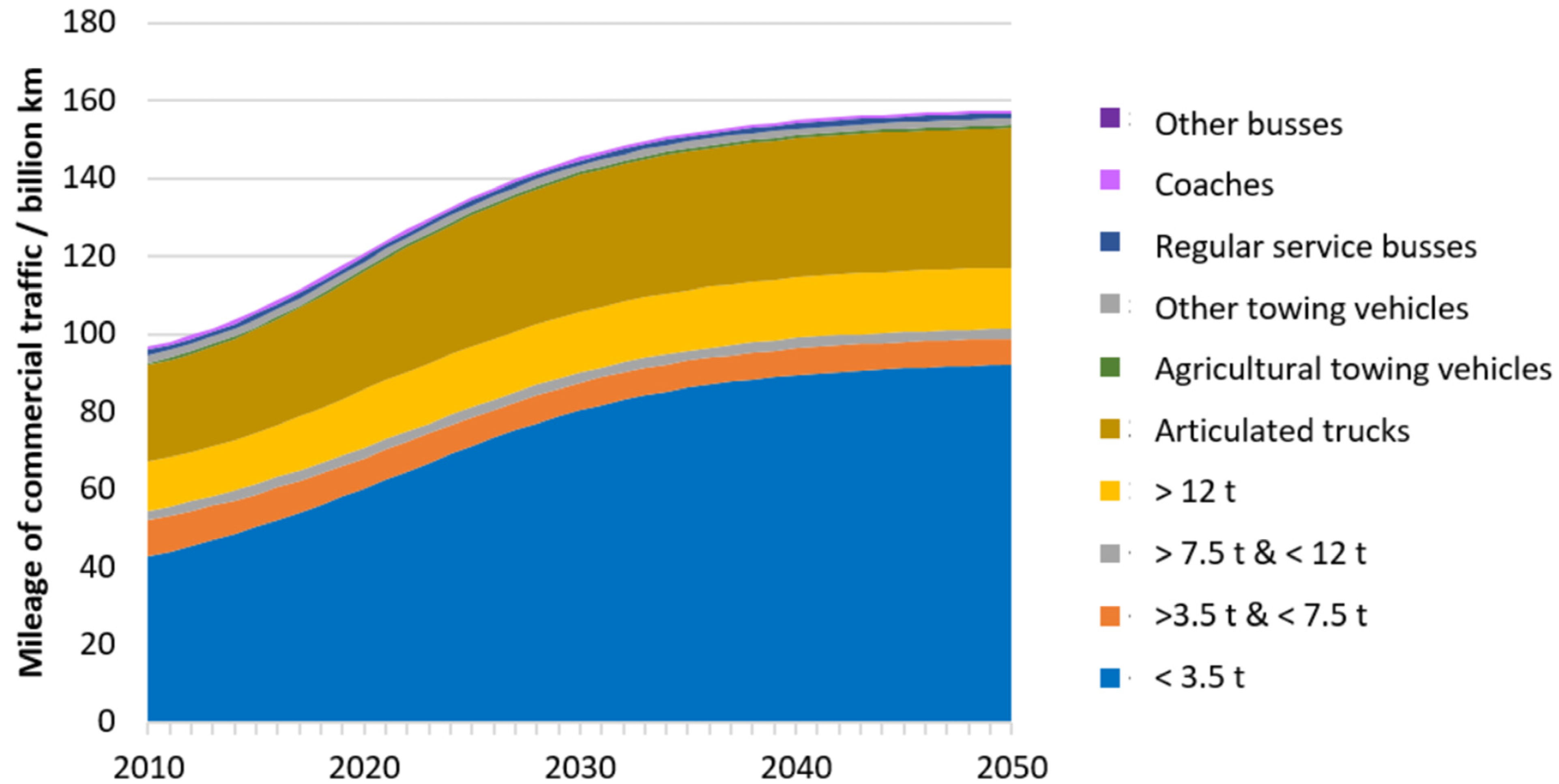
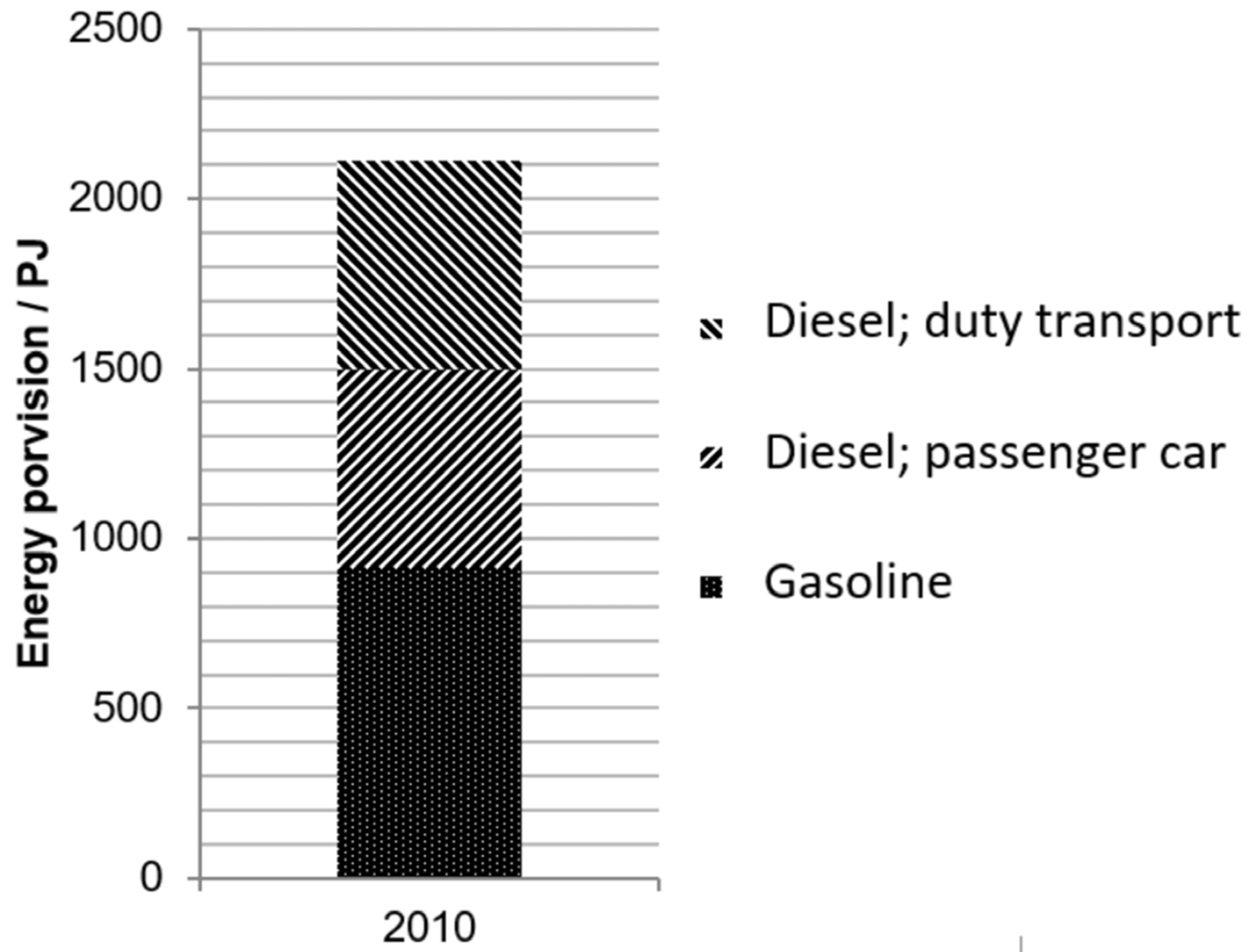
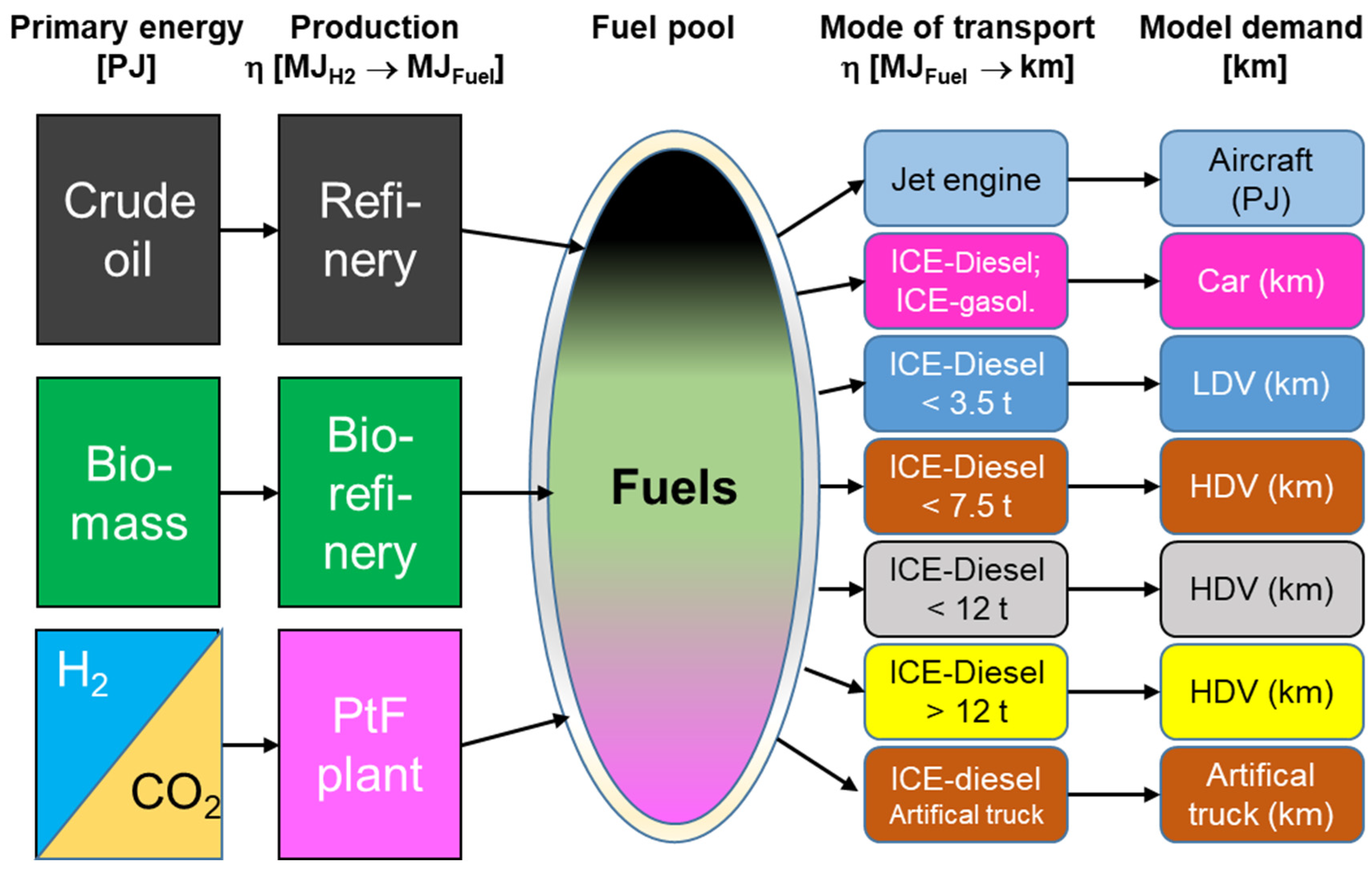
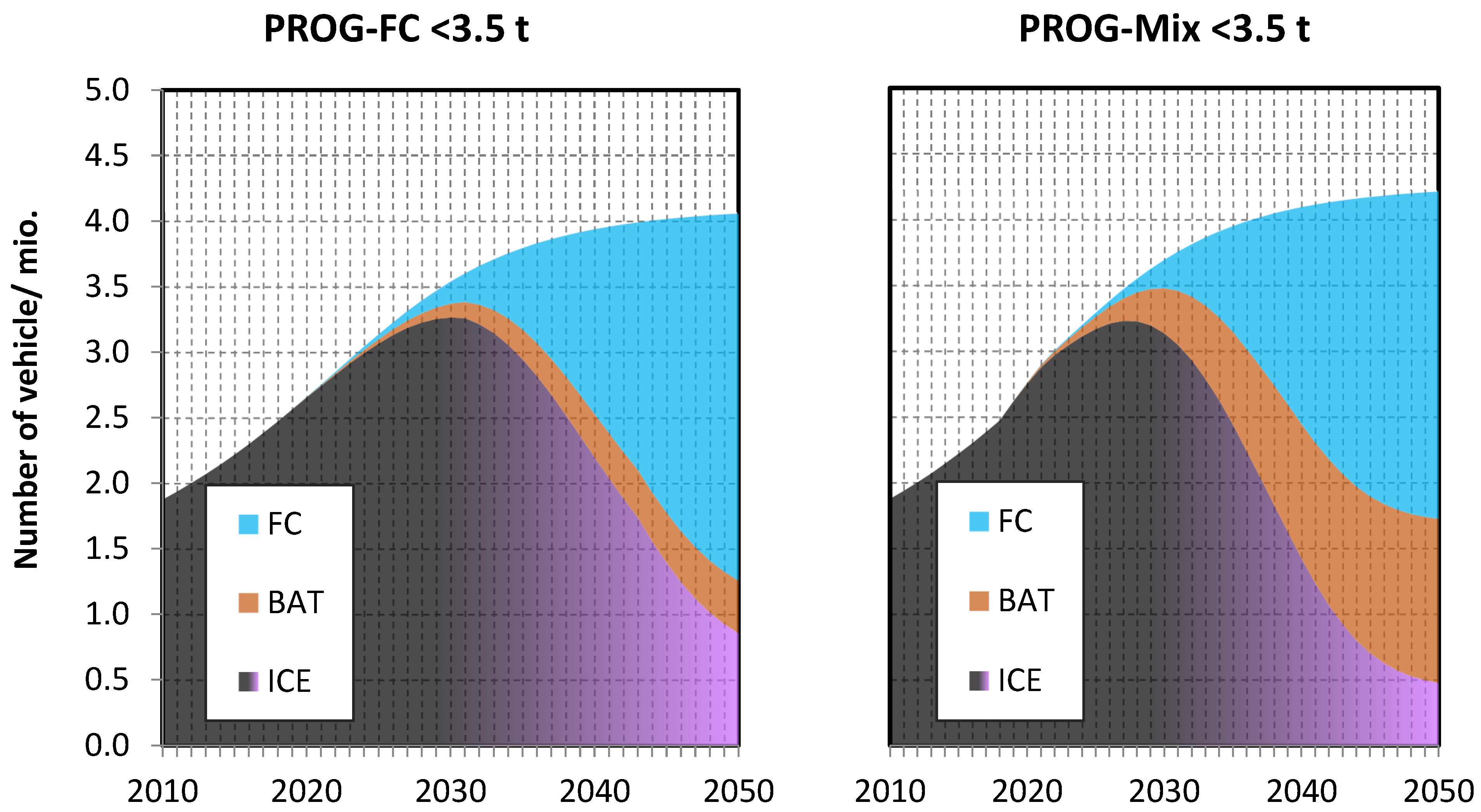
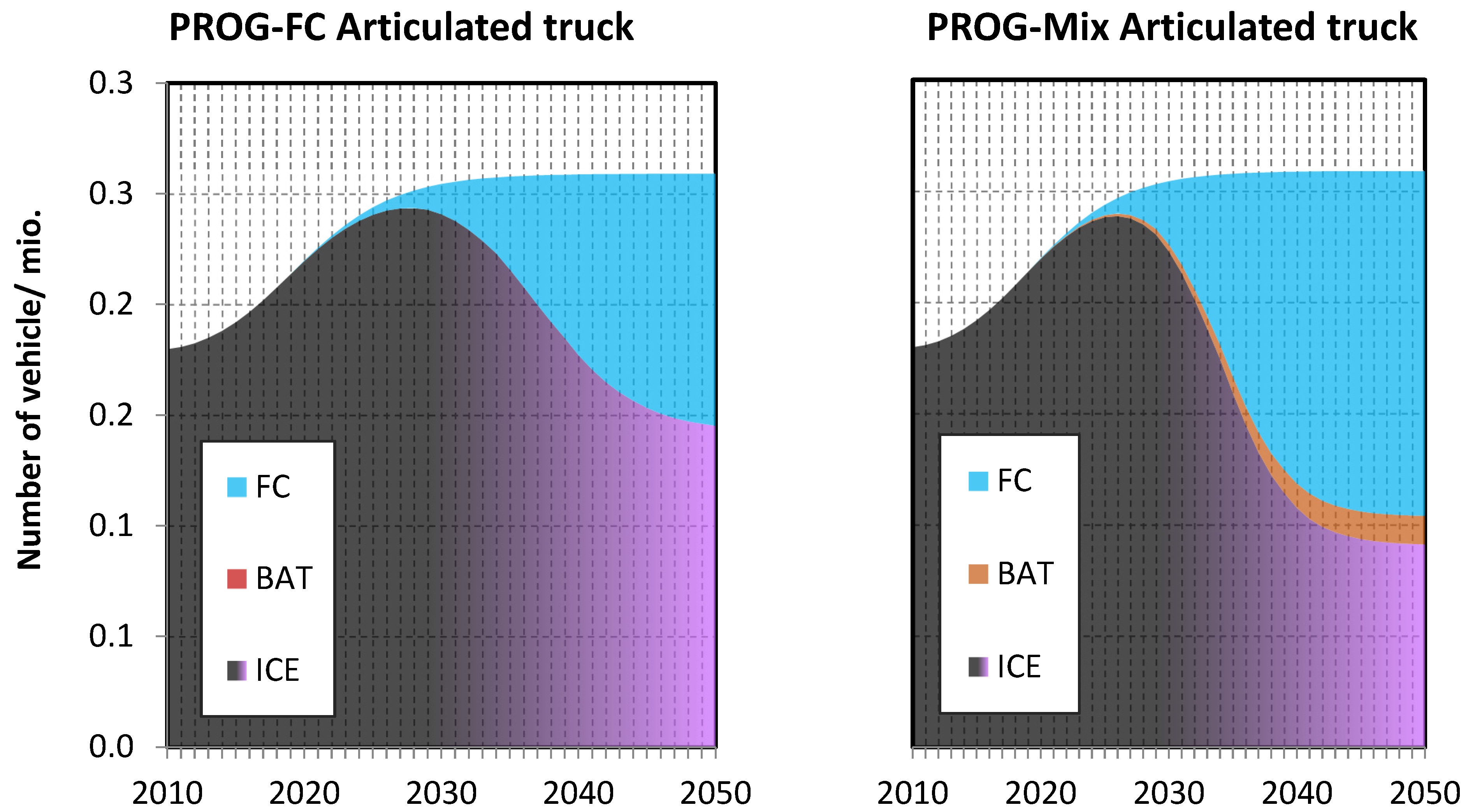
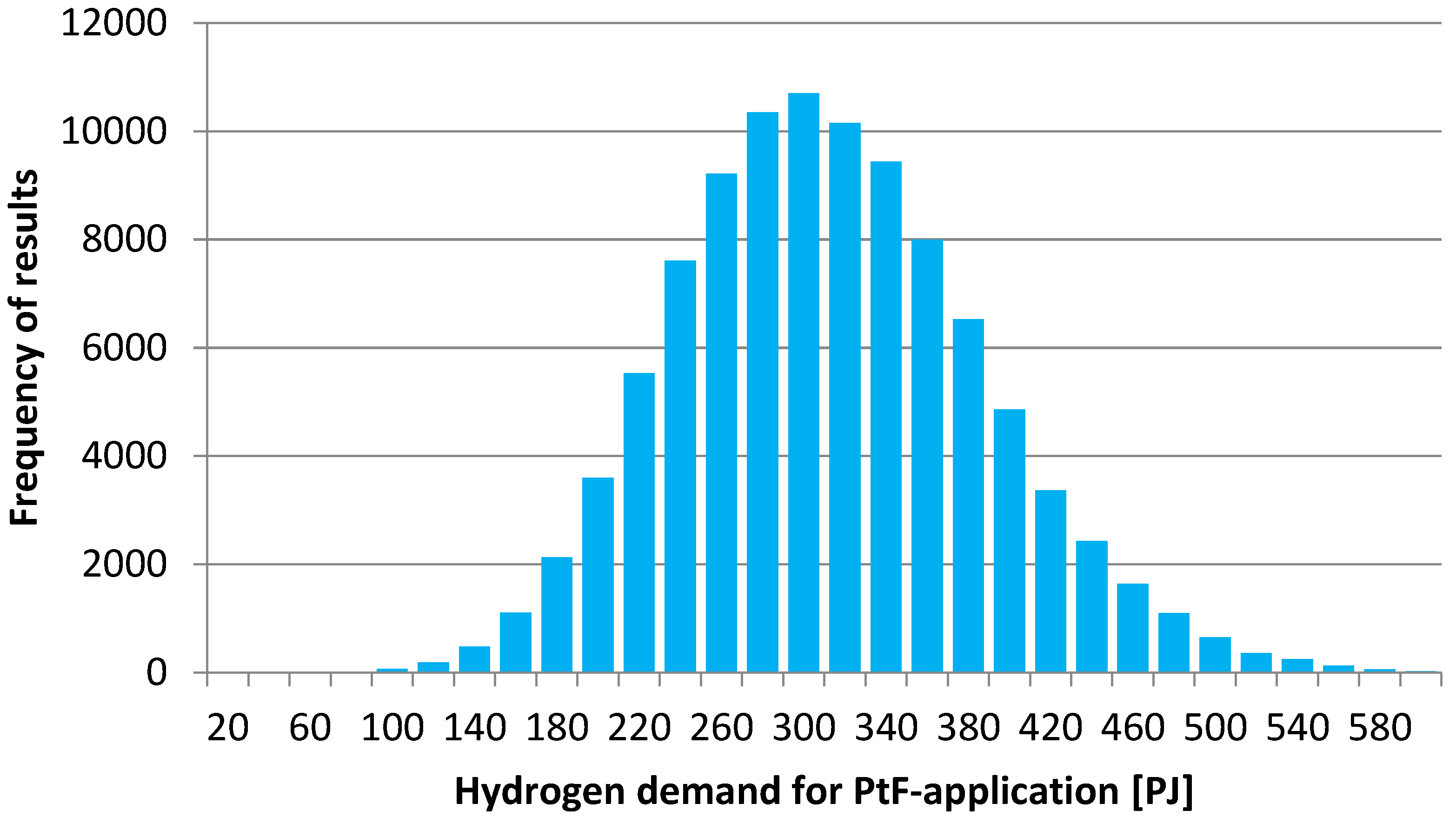
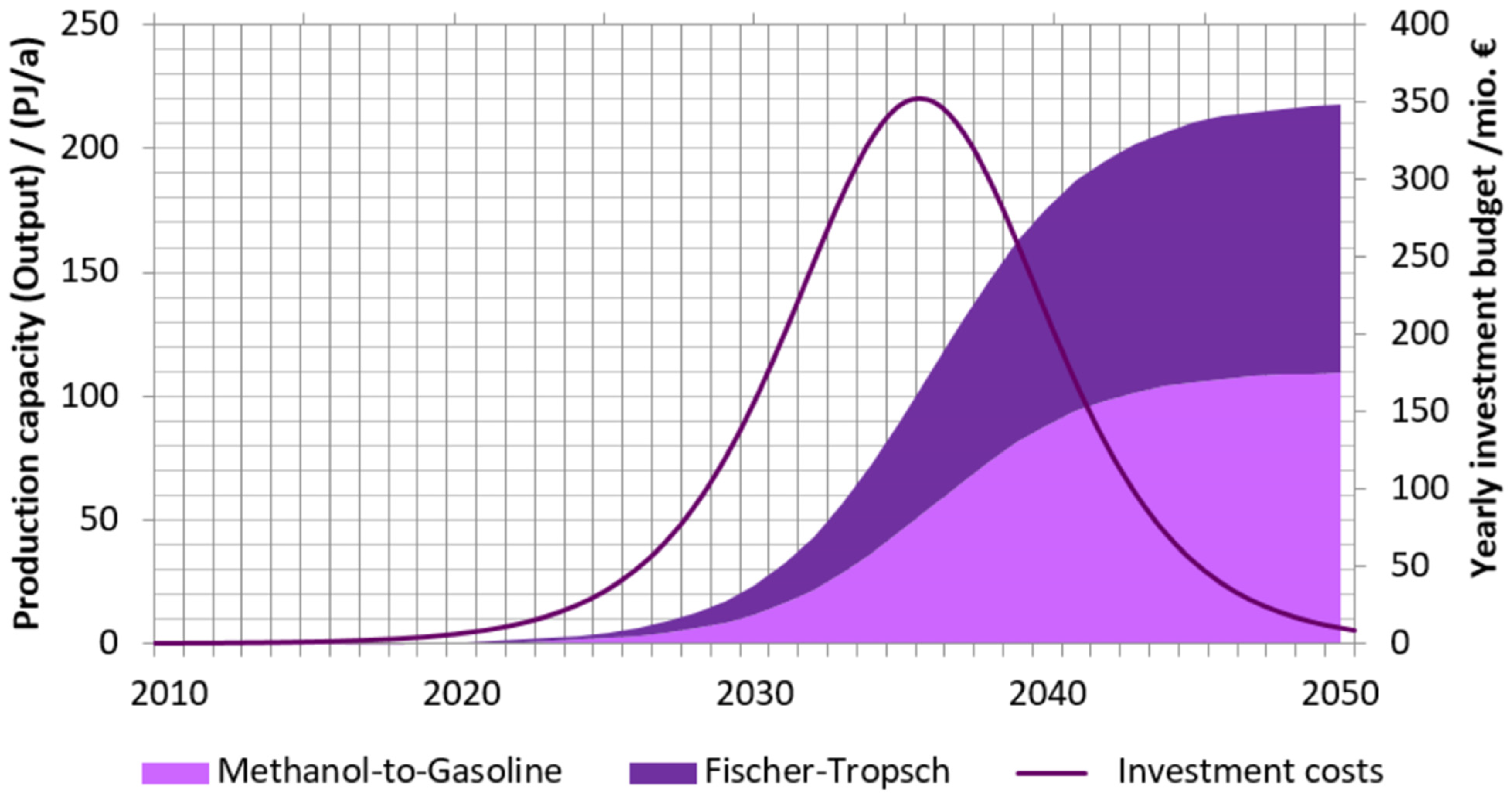
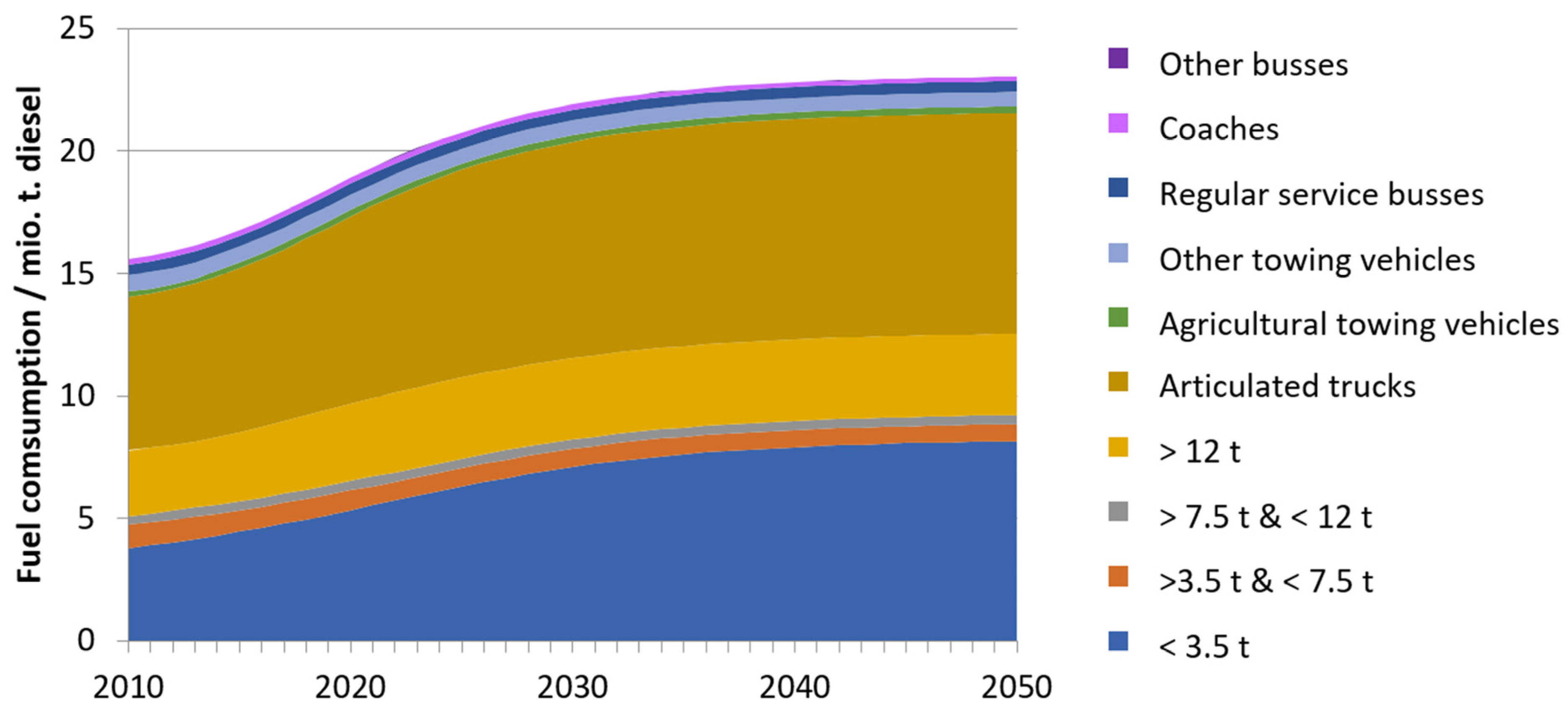
Table A1.
Average factors for calculation of the scenario indicators in Table A2.
Table A1.
Average factors for calculation of the scenario indicators in Table A2.
| Loading | Average Mileage | Fuel Demand | Stock | Mileage Share of Trips Abroad | Fuel Behavior | Unassigned Consumption | |||
|---|---|---|---|---|---|---|---|---|---|
| [14] | [14,84] | [85] | [39] | [52,55] | [53] | [53] | |||
| Share of Fueled to Driven Distance From… | |||||||||
| Nationals Abroad | Foreigners Inland | Nationals Abroad | Foreigners Inland | ||||||
| [t] | [km/a] | [MJ/100 km] | [Nos.] | [%] | [%] | [%] | [%] | [%] | |
| <3.5 t | 0.2 | 19,388 | 380 | 1,909,209 | 2.99 | 6.18 | 200 | 50 | 0 |
| <7.5 t | 0.3 | 25,000 | 440 | 271,403 | 2.25 | 37.69 | 200 | 50 | 14 |
| <12 t | 2.7 | 25,000 | 620 | 71,890 | 2.00 | 39.56 | 200 | 50 | 14 |
| >12 t | 5.5 | 50,000 | 920 | 188,832 | 1.84 | 34.80 | 200 | 50 | 14 |
| AT | 13.5 | 100,899 | 1080 | 178,050 | 6.57 | 43.80 | 200 | 50 | 16 |
| Bus | 0 | 1200 | 4.29 | 6.06 | 200 | 50 | 0 | ||
Table A2.
Results of the scenario key figures for the year 2010, calculated from the inventory data from the statistics of the KBA [39].
Table A2.
Results of the scenario key figures for the year 2010, calculated from the inventory data from the statistics of the KBA [39].
| Calculation of Drive Performance | ||||||||
|---|---|---|---|---|---|---|---|---|
| Stock | National | Aborad/Foreigns | National Demand | Fuel Behavior | Fuel Sales | |||
| National Abroad | Foreigns Inland | National Abroad | Foreigns Inland | |||||
| [Vehicles] | [Mil. km] | [Mil. km] | [Mil. km] | [Mil. km] | [Mil. km] | [Mil. km] | [Mil. km] | |
| <3.5 t | 1.909.209 | 37.02 | 1.11 | 2.29 | 38.20 | −2.21 | 1.14 | 35.95 |
| <7.5 t | 271.403 | 6.79 | 0.15 | 2.56 | 9.19 | −0.30 | 1.28 | 7.76 |
| <12 t | 71.890 | 1.80 | 0.04 | 0.71 | 2.47 | −0.07 | 0.36 | 2.08 |
| >12 t | 188.832 | 9.44 | 0.17 | 3.29 | 12.55 | −0.35 | 1.64 | 10.74 |
| AT | 178.050 | 17.97 | 1.18 | 7.87 | 24.65 | −2.36 | 3.93 | 19.54 |
| Bus | 3.96 | 0.17 | 0.24 | 4.03 | −0.34 | 0.12 | 3.74 | |
| Total | 76.96 | 2.82 | 16.95 | 91.10 | −5.64 | 8.48 | 79.80 | |
AT: articulated truck.
Table A3.
Results of the key scenario figures for the year 2010, calculated from the inventory data from the statistics of the KBA [39] (Table A2 continued).
| Calculation of Fuel Quantities | |||||||||
|---|---|---|---|---|---|---|---|---|---|
| Stock | National | National Demand | Sales | Transport Performance | |||||
| UC * | with UC * | with UC * | with UC * | National | |||||
| [Vehicles] | [Mt/a] | [Mt/a] | [Mt/a] | [Mt/a] | [Mt/a] | [Mt/a] | [Mt/a] | [Mrd. tkm] | |
| <3.5 t | 1.909.209 | 3.27 | 0.00 | 3.27 | 3.38 | 3.38 | 3.18 | 3.18 | 8.67 |
| <7.5 t | 271.403 | 0.69 | 0.10 | 0.79 | 0.94 | 1.04 | 0.79 | 0.89 | 2.76 |
| <12 t | 71.890 | 0.26 | 0.04 | 0.30 | 0.36 | 0.39 | 0.30 | 0.34 | 6.67 |
| >12 t | 188.832 | 2.02 | 0.28 | 2.30 | 2.69 | 2.97 | 2.30 | 2.58 | 69.04 |
| AT | 178.050 | 4.51 | 0.72 | 5.23 | 6.19 | 6.91 | 4.91 | 5.63 | 332.82 |
| Bus | 1.11 | 0.00 | 1.11 | 1.12 | 1.12 | 1.04 | 1.04 | 0.00 | |
| Total | 11.86 | 1.14 | 13.0 | 14.67 | 15.81 | 12.52 | 13.66 | 419.96 | |
* Unassigned consumption (UC), AT: articulated truck.
Table A4.
S-curve parameters to describe the new registration structure of commercial vehicles according to classes in the PROG–FC scenario.
Table A4.
S-curve parameters to describe the new registration structure of commercial vehicles according to classes in the PROG–FC scenario.
| FCEVs | BEVs | |||||
|---|---|---|---|---|---|---|
| <3.5 t | 2035 | 75 | 300 | 2028 | 10 | 300 |
| <12 t | 2035 | 75 | 300 | 2028 | 10 | 300 |
| >12 t | 2035 | 45 | 300 | - | - | - |
| Articulated trucks | 2035 | 45 | 300 | - | - | - |
| Regular-service buses | 2030 | 50 | 300 | 2030 | 10 | 300 |
| Coaches | 2032 | 45 | 300 | - | - | - |
| Others | 2040 | 10 | 300 | - | - | - |
Table A5.
S-curve parameters to describe the new registration structure of commercial vehicles according to classes in the PROG–Mix scenario.
Table A5.
S-curve parameters to describe the new registration structure of commercial vehicles according to classes in the PROG–Mix scenario.
| FCEVs | BEVs | |||||
|---|---|---|---|---|---|---|
| <3.5 t | 2032 | 60 | 400 | 2028 | 30 | 300 |
| <12 t | 2032 | 40 | 400 | 2028 | 30 | 300 |
| >12 t | 2032 | 50 | 400 | 2032 | 10 | 300 |
| Articulated trucks | 2032 | 60 | 400 | 2032 | 5 | 300 |
| Regular-service buses | 2030 | 75 | 400 | 2030 | 20 | 300 |
| Coaches | 2032 | 50 | 400 | 2032 | 10 | 300 |
| Others | 2040 | 10 | 400 | 2030 | 10 | 300 |
Table A6.
S-curve parameters to describe the new car registration structure in two electrification scenarios.
Table A6.
S-curve parameters to describe the new car registration structure in two electrification scenarios.
| FCEVs | BEVs | |||||
|---|---|---|---|---|---|---|
| PROG–FC | 2033 | 45 | 300 | 2024 | 28 | 300 |
| PROG–Mix | 2035 | 60 | 400 | 2028 | 25 | 400 |
Table A7.
Curve parameters and standard deviation from S-curve fitting to chemical industrial production growth stages based on historical data.
Table A7.
Curve parameters and standard deviation from S-curve fitting to chemical industrial production growth stages based on historical data.
| Ethylen 1962–1990 | Ethylen 1987–2016 | Propylen 1975–2010 | |
|---|---|---|---|
| 0.00 | 3.00 | 1.60 | |
| 3.03 | 2.10 | 1.95 | |
| 1968 | 1995 | 1995 | |
| 2.85 | 2.00 | 2.00 | |
| 0.256 | 0.253 | 0.193 |
Table A8.
S-curve parameters chosen to describe the development of the PtF production capacities.
| Case 1 (Red) | Case 2 (Blue) | |
| 0 | 0 | |
| 5.1 | 5.1 | |
| 2036 | 2032 | |
| 2.85 | 2.00 |
References
- Commission Welcomes Completion of Key ‘Fit for 55’ Legislation, Putting EU on Track to Exceed 2030 Targets. Available online: https://ec.europa.eu/commission/presscorner/detail/en/IP_23_4754 (accessed on 29 February 2024).
- Peters, R.; Breuer, J.L.; Decker, M.; Grube, T.; Robinius, M.; Samsun, R.C.; Stolten, D. Future Power Train Solutions for Long-Haul Trucks. Sustainability 2021, 13, 2225. [Google Scholar] [CrossRef]
- Bründlinger, T.; König, J.E.; Gründig, D.; Frank, O.; Jugel, C.; Kraft, P.; Krieger, O.; Mischinger, S.; Prein, P.; Seidl, H.; et al. Leitstudie Integrierte Energiewende; Deutsche Energie-Agentur GmbH: Dena, Germany, 2018. [Google Scholar]
- Decker, M. Strategieentwicklung zur Umsetzung der Klimaschutzziele im Verkehrssektor mit dem Fokus Kraftstoffe; RWTH University of Aachen: Aachen, Germany, 2023. [Google Scholar]
- Harrison, P. Fuelling Europe’s Future: How the Transition from Oil Strengthens the Economy; Cambridge Econometrics: Cambridge, UK, 2018. [Google Scholar]
- Christensen, A.; Petrenko, C. CO2-Based Synthetic Fuel: Assessment of Potential European Capacity and Environmental Performance; The International Council on Clean Transportation (ICCT): Washington DC, USA, 2017. [Google Scholar]
- Siegemund, S.; Schmidt, P.; Trommler, M.; Weindorf, W.; Kolb, O.; Werner, Z.; Zinnecker, V.; Raksha, T.; Zerhusen, J. “E-Fuels”-Study the Potential of Electricity Based Fuels for Low-Emission Transport in the EU.; Deutsche Energie-Agentur GmbH: Dena, Germany, 2017. [Google Scholar]
- International Aspects of A Power-to-X Roadmap—A Report Prepared for The World Energy Council Germany; World Energy Council Germany: Berlin, Germany, 2018.
- Die Zukünftigen Kosten Strombasierter Synthetischer Brennstoffe: Schlussfolgerungen aus Sicht von Agora Verkehrswende und Agora Energiewende; Agora Verkehrswende und Agora Energiewende: Berlin, Germany, 2018.
- Pfennig, M.; Gerhardt, N.; Carsten, P.; Böttger, D. Mittel- und Langfristige Potenziale von PtL- und H2-Importen aus Internationalen EE-Vorzugsregionen; Fraunhofer-Institut für Windenergie und Energiesystemtechnik: Bremerhaven, Germany, 2017. [Google Scholar]
- Flachsbarth, F.; Kasten, P. Aktuelle Potenziale der Produktion von PtX-Kraftstoffen auf Basis von Zusätzlich Integrierten Erneuerbaren Energien; Öko-Institut e.V.: Freiburg im Breisgau, Germany, 2017. [Google Scholar]
- Pietzcker, R.; Longden, T.; Chen, W.; Fu, S.; Kriegler, E.; Kyle, P.; Luderer, G. Long-Term Transport Energy Demand and Climate Policy: Alternative Visions on Transport Decarbonization in Energy Economy Models. Energy 2013, 64, 95–108. [Google Scholar] [CrossRef]
- Schnülle, C.; Gleich, A.; Goessling-Reisemann, S.; Kisjes, K.; Nikolic, I.; Stührmann, T.; Thier, P. Optionen für die Integration von Power-to-Fuel in den Energiewendeprozess aus einer sozioökonomischen Perspektive. Vierteljahrsh. Zur Wirtsch. 2016, 85, 53–74. [Google Scholar] [CrossRef]
- Schmidt, P.; Zittel, W.; Weindorf, W.; Rakasha, T.; Goericke, D. Renewables in Transport 2050—Empowering a Sustainable Mobility Future with Zero Emission Fuels; LBST, Ludwig Bölkow Systemtechnik—Forschungsvereinigung Verbrennungsmaschinen e.V.: Frankfurt am Main, Germany, 2016. [Google Scholar]
- Kreyenberg, D.; Lischke, A.; Bergk, F.; Duennebeil, F.; Heidt, C.; Knörr, W.; Raksha, T.; Schmidt, P.; Weindorf, W.; Naumann, K.; et al. Erneuerbare Energien im Verkehr—Potenziale und Entwicklungsperspektiven Verschiedener Erneuerbarer Energieträger und Energieverbrauch der Verkehrsträger; Bundesministerium für Verkehr und digitale Infrastruktur (BMVI); Deutsches Zentrum für Luft- und Raumfahrt e.V.; Institut für Energie- und Umweltforschung Heidelberg GmbH; Ludwig-Bölkow-Systemtechnik GmbH; Deutsches Biomasseforschungszentrum GmbH: Berlin, Germany, 2016. [Google Scholar]
- Knörr, W.; Heidt, C.; Gores, S.; Bergk, F. Aktualisierung, Daten- und Rechenmodell: Energieverbrauch und Schadstoffemissionen des mo-Torisierten Verkehrs in Deutschland 1960–2035: (TREMOD) für die Emissionsberichterstattung 2016 (Berichtsperiode 1990–2014); Ifeu-Institut für Energie- und Umweltforschung Heidelberg GmbH, Öko-Institut: Freiburg im Breisgau, Germany, 2016. [Google Scholar]
- Bergk, F.; Biemann, K.; Heidt, C.; Knörr, W.; Lambrecht, U.; Schmidt, T.; Ickert, L.; Schmied, M.; Schmidt, P.; Weindorf, W. Klimaschutzbeitrag des Verkehrs bis 2050; ifeu—Institut für Energie- und Umweltforschung Heidelberg GmbH, INFRAS AG, LBST-Ludwig-Bölkow-Systemtechnik GmbH: Ottobrunn, Germany, 2016. [Google Scholar]
- Schlesinger, D.M.; Hofer, P.; Kemmler, D.A.; Kirchner, D.A.; Strassburg, S. Energieszenarien für ein Energiekonzept der Bundesregierung; Prognos AG, EWI—Energiewirtschaftliches Institut an der Universität zu Köln, Gesellschaft für Wirtschaftliche Strukturforschung mbH (GWS): Osnabrück, Germany, 2010. [Google Scholar]
- Kasten, P.; Mottschall, M.; Köppel, W.; Degünther, C.; Schmied, M.; Wüthrich, P. Erarbeitung Einer Fachlichen Strategie zur Energieversorgung des Verkehrs bis Zum Jahr 2050; Umweltbundesamt (UBA), Öko-Institut e.V., DVGW-Forschungsstelle am Engler-Bunte-Institut des Karlsruher Instituts für Technologie (KIT), INFRAS AG: Freiburg im Breisgau, Germany, 2016. [Google Scholar]
- Zimmer, W.; Blanck, R.; Bergmann, T.; Mottschall, M.; von Waldenfels, R.; Förster, H. Endbericht Renewbility III—Optionen Einer Dekarbonisierung des Verkehrssektors; Öko-Institut e.V.: Freiburg im Breisgau, Germany, 2017. [Google Scholar]
- Hacker, F.; Blanck, R.; Hülsmann, F.; Kasten, P.; Loreck, C.; Ludig, S.; Mottschall, M.; Zimmer, W. eMobil 2050—Szenarien Zum möglichen Beitrag des elektrischen Verkehrs zum Langfristigen Klimaschutz; Öko-Institut e.V.: Freiburg im Breisgau, Germany, 2014. [Google Scholar]
- Lischke, A.; Windmüller, D.; Wurster, R.; Weindorf, W.; Heidt, C.; Naumann, K. Identifizierung von Hemmnissen der Nutzung von LNG und CNG im Schweren Lkw-Verkehr Sowie Möglichkeiten zu Deren Überwindung; Bundesministeriums für Verkehr und digitale Infrastruktur (BMVI), Deutsches Zentrum für Luft- und Raumfahrt e.V. (DLR), ifeu—Institut für Energie- und Umweltforschung Heidelberg GmbH, Ludwig-Bölkow-Systemtechnik GmbH (LBST), Deutsches Biomasseforschungszentrum gGmbH (DBFZ): Leipzig, Germany, 2015. [Google Scholar]
- Sterner, M.; Thema, M.; Eckert, F.; Moser, A.; Schäfer, A.; Drees, T.; Rehtanz, C.; Häger, U.; Kays, J.; Seack, A.; et al. Stromspeicher in der Energiewende; Agora Energiewende, FENES Forschungsstelle für Energie-netze und Energiespeicher, IAEW Institut für Elektrische Anlagen und Energie-wirtschaft, ef.Ruhr GmbH, ISEA Institut für Stromrichtertechnik und Elektrische Antriebe: Aachen, Germany, 2014. [Google Scholar]
- Ramesohl, S.; Fischedick, M.; Arnold, K.; Merten, F.; Nitsch, J.; Schmid, S.; Viebahn, P.; Pehnt, M.; Knörr, W.; Gärtner, S.; et al. Entwicklung Einer Gesamtstrategie zur Einführung Alternativer Kraftstoffe, Insbesondere Regenerativ Erzeugten Wasserstoffs; Wuppertal Institut für Klima Umwelt Energie, Deutsches Zentrum für Luft-und Raumfahrt (DLR), Institut für Energie und Umweltforschung (IFEU): Heidelberg, Germany, 2006. [Google Scholar]
- Nationaler Strategierahmen über den Aufbau der Infrastruktur für Alternative Kraftstoffe; Bundesministerium für Verkehr und digitale Infrastruktur (BMVI): Berlin, Germany, 2017.
- Zech, K.; Naumann, K.; Müller-Langer, F.; Schmidt, P.; Weindorf, P.; Mátra, Z.; Grimme, W.; Hepting, M.; Heidt, C. Drop in Kraftstoffe für die Luftfahrt; Bundesministerium für Verkehr und digitale Infrastruktur (BMVI); Deutsches Zentrum für Luft- und Raumfahrt e.V.; Institut für Energie- und Umweltforschung Heidelberg GmbH; Ludwig-Bölkow-Systemtechnik GmbH; Deutsches Biomasseforschungszentrum GmbH: Berlin, Germany, 2014. [Google Scholar]
- Alonso, M.; Arias, B.; Marbán, G.; Turrado, S.; Abanades, C. D12.1 Results from 30 kWth CaL CFB Experiments (M18); CEMCAP: Dusseldorf, Germany, 2016. [Google Scholar]
- Hobohm, J.; Dambeck, H.; Falkenberg, H.; Kemmler, D.A.; Koziel, S.; Wendring, P.; Ziegenhagen, I.; Meyer, B.; Dotzauer, M. Status und Perspektiven flüssiger Energieträger in der Energiewende; Prognos AG: Frankfurt am Main, Germany, 2017. [Google Scholar]
- Purr, K.; Osiek, D.; Lange, M.; Adlunger, K. Integration von Power to Gas/Power to Liquid in den laufenden Transformationsprozess; Umweltbundesamt: Berlin, Germany, 2016. [Google Scholar]
- Arnold, K.; Kobiela, G.; Pastowski, A. Technologiebericht 4.3 Power-to-Liquids/-Chemicals Innerhalb des Forschungsprojekts TF_Energiewende; Wuppertal Institut für Klima, Umwelt, Energie: Wuppertal, Germany, 2018. [Google Scholar]
- Adolf, J.; Balzer, C.; Haase, F.; Lenz, B.; Lischke, A.; Knitschky, G. Shell Nutzfahrzeug-Studie—Diesel Oder Alternative Antriebe —Womit Fahren Lkw Und Bus Morgen? Shell Deutschland, Deutsches Zentrum für Luft- und Raumfahrt (DLR): Cologne, Germany, 2016. [Google Scholar]
- Adolf, J.; Rommerskirchen, S. Shell PKW-Szenarien bis 2040: Fakten, Trends und Perspektiven für Auto-Mobilität; Shell Deutschland Oil: Hamburg, Germany, 2014. [Google Scholar]
- Gnann, T.; Wietschel, M.; Kühn, A.; Thielmann, A.; Sauer, A.; Plötz, P.; Moll, C.; Stütz, S.; Schellert, M.; Rüdiger, D.; et al. Teilstudie "Brennstoffzellen-LKW: Kritische Entwicklungshemmnisse, Forschungsbedarf und Marktpotential": Wissenschaftliche Beratung des BMVI zur Mobilitäts- und Kraftstoffstrategie; Fraunhofer ISI, Fraunhofer IML, PTV Transport Consult GmbH: Karlsruhe, Germany, 2017. [Google Scholar]
- Wietschel, M.; Gnann, T.; Kühn, A.; Plötz, P.; Moll, C.; Speth, D.; Buch, J.; Boßmann, T. Machbarkeitsstudie zur Ermittlung der Potentiale des Hybrid-Oberleitungs-Lkw: Studie im Rahmen der Wissenschaftlichen Beratung des BMVI zur Mobilitäts- und Kraftstoffstrategie; Bundesministerium für Verkehr und Digitale Infrastruktur (BMVI), Fraunhofer ISI, Fraunhofer IML, PTV Transport Consult GmbH, TU Hamburg-Harburg—IUE, M-Five: Karlsruhe, Germany, 2017. [Google Scholar]
- Adolf, J.; Balzer, C.H.; Louis, J.; Schabla, U.; Fischedick, M.; Arnold, K.; Pastowski, A.; Schüwer, D. Energie der Zukunft? Nachhaltige Mobilität durch Brennstoffzelle und H2; Shell Wasserstoff-Studie; Shell Deutschland, Wuppertal Institut für Klima, Umwelt, Energie: Wuppertal, Germany, 2017. [Google Scholar]
- Die Rolle von Batteriebetriebenen Elektrofahrzeugen, Plug-in Hybridfahrzeugen und Brennstoffzellenfahrzeugen: Ein Portfolio von Antriebssystemen für Europa: Eine Faktenbasierte Analyse; NOW Nationale Organisation Wasserstoff- und Brennstoffzellentechnologie: Berlin, Germany, 2015.
- Altenburg, S.; der Maur, A.A.; Labinsky, A.; Eckert, S.; Faltenbacher, M.; Reuter, B. Nullemissionsnutzfahrzeuge: Vom Ökologischen Hoffnungsträger zur Ökonomischen Alternative; e-mobil BW GmbH: Stuttgart, Germany, 2017. [Google Scholar]
- Dünnbeil, F.; Lambrecht, U.; Goletz, M.; Zittel, W.; Schmidt, P.; Müller-Langer, F.; Naumann, K. Kurzstudie: Analyse aktueller Szenarien zur Entwicklung des Verkehrs in Deutschland und dessen Umweltwirkungen; BMVBS (Bundesministerium für Verkehr, Bau und Stadtentwicklung, DLR (Deutsches Zentrum für Luft- und Raumfahrt), IFEU (Institut für Energie- und Umweltforschung), LBST (Ludwig-Bölkow-Systemtechnik) und DBFZ (Deutsches Biomasseforschungszentrum): Berlin, Germany, 2013. [Google Scholar]
- Fahrzeugzulassungen (FZ): Bestand an Nutzfahrzeugen, Kraftfahrzeugen Insgesamt und Kraftfahrzeuganhängern nach Technischen Daten (Größenklassen, Motorisierung, Fahrzeugklassen und Aufbauarten) FZ 25; Kraftfahrtbundesamt (KBA): Flensburg, Germany, 2017.
- Li, L.; Wang, B.; Jiao, K.; Ni, M.; Du, Q.; Liu, Y.; Li, B.; Ling, G.; Wang, C. Comparative techno-economic analysis of large-scale renewable energy storage technologies. Energy AI 2023, 14, 100282. [Google Scholar] [CrossRef]
- Welder, L.; Ryberg, D.S.; Kotzur, L.; Grube, T.; Robinius, M.; Stolten, D. Spatio-temporal optimization of a future energy system for power-to-hydrogen applications in Germany. Energy 2018, 158, 1130–1149. [Google Scholar] [CrossRef]
- Schemme, S.; Breuer, J.L.; Köller, M.; Meschede, S.; Walman, F.; Samsun, R.C.; Peters, R.; Stolten, D. H2-based synthetic fuels: A techno-economic comparison of alcohol, ether and hydrocarbon production. Int. J. Hydrogen Energy 2020, 45, 5395–5414. [Google Scholar] [CrossRef]
- Schemme, S.; Samsun, R.C.; Peters, R.; Stolten, D. Power-to-fuel as a key to sustainable transport systems—An analysis of diesel fuels produced from CO2 and renewable electricity. Fuel 2017, 205, 198–221. [Google Scholar] [CrossRef]
- Brynolf, S.; Hansson, J.; Anderson, J.E.; Skov, I.R.; Wallington, T.J.; Grahn, M.; Korberg, A.D.; Malmgren, E.; Taljegård, M. Review of electrofuel feasibility—Prospects for road, ocean, and air transport. Prog. Energy 2022, 4, 042007. [Google Scholar] [CrossRef]
- Brynolf, S.; Taljegard, M.; Grahn, M.; Hansson, J. Electrofuels for the transport sector: A review of production costs. Renew. Sustain. Energy Rev. 2018, 81, 1887–1905. [Google Scholar] [CrossRef]
- Grahn, M.; Malmgren, E.; Korberg, A.D.; Taljegard, M.; Anderson, J.E.; Brynolf, S.; Hansson, J.; Skov, I.R.; Wallington, T.J. Review of electrofuel feasibility—Cost and environmental impact. Prog. Energy 2022, 4, 032010. [Google Scholar] [CrossRef]
- Hansson, J.; Hackl, R.; Taljegard, M.; Brynolf, S.; Grahn, M. The Potential for Electrofuels Production in Sweden Utilizing Fossil and Biogenic CO2 Point Sources. Front. Energy Res. 2017, 5, 4. [Google Scholar] [CrossRef]
- Schnuelle, C.; Kisjes, K.; Stuehrmann, T.; Thier, P.; Nikolic, I.; von Gleich, A.; Goessling-Reisemann, S. From Niche to Market—An Agent-Based Modeling Approach for the Economic Uptake of Electro-Fuels (Power-to-Fuel) in the German Energy System. Energies 2020, 13, 5522. [Google Scholar] [CrossRef]
- Pengg, H. Marktchancen Erkennen—Erfolgreiche Marktprognosen mit Hilfe der S-Kurven-Methode; Wirtschaftsuniversität Wien: Vienna, Austria; Haupt-Verlag: Bern, Switzerland, 2003. [Google Scholar]
- Marchetti, C.; Nakicenovic, N. The Dynamics of Energy Systems and the Logistic Substitution Model; IIASA, Laxenburg, Austria, 1979.
- Harrer, G. Das Vester’sche Sensitivitätsmodell. In Komplexitätsmanagement; Fisch, R., Beck, D., Eds.; VS Verlag für Sozialwissenschaften: Wiesbaden, Germany, 2004. [Google Scholar] [CrossRef]
- Bäumer, M.; Hautzinger, H.; Pfeiffer, M.; Stock, W.; Lenz, B.; Kuhnimhof, T.; Köhler, K. Fahrleistungserhebung 2014—Inlandsfahrleistung und Unfallrisiko (V 291); Bundesanstalt für Straßenwesen (Bast), IVT Research GmbH, Institut für Verkehrsforschung DLR: Berlin, Germany, 2014. [Google Scholar]
- Mayer, H.; Fehrentz, P. Umweltökonomische Gesamtrechnunge—Weiterentwicklung der Berechnungen zum Energieverbrauch und zu den CO2-Emissionen des Straßenverkehrs im Rahmen des NAMEA Rechenansatzes—Methodenbericht; Statistisches Bundesamt: Wiesbaden, Germany, 2011. [Google Scholar]
- Schubert, M.; Kluth, T.; Nebauer, G.; Ratzenberger, R.; Kotzagiorgis, S.; Butz, B.; Schneider, W.; Leible, M. Verkehrsverflechtungsprognose 2030; Bundesministerium für Verkehr und digitale Infrastruktur, Intraplan Consult GmbH, BVU Beratergruppe Verkehr+Umwelt GmbH: Berlin, Germany, 2014. [Google Scholar]
- Bäumer, M.; Hautzinger, H.; Pfeiffer, M.; Stock, W.; Lenz, B.; Kuhnimhof, T.; Köhler, K. Fahrleistungserhebung 2014—Inländerfahrleistung (V 290); Bundesanstalt für Straßenwesen (bast), IVT Research GmbH, Institut für Verkehrsforschung DLR: Berlin, Germany, 2014. [Google Scholar]
- Jahresbericht 2018; Mineralölwirtschaftsverband e.V. (MWV): Berlin, Germany, 2018.
- Schmidt, N.; Kille, C.; Schroer, B.; Wandel, A. Wirtschaftliche Rahmenbedingungendes Güterverkehrs; Fraunhofer ATL, KPMG: Berlin, Germany, 2008. [Google Scholar]
- Robinius, M.; Linßen, J.; Grube, T.; Reuß, M.; Stenzel, P.; Syranidis, K.; Kuckertz, P.; Stolten, D. Comparative Analysis of Infrastructures: Hydrogen Fueling and Electric Charging of Vehicles; Series Energy & Environment; Forschungszentrum Jülich GmbH: Jülich, Germany, 2018; Volume 408, ISBN 978-3-95806-295-5. [Google Scholar]
- Reuss, M. Techno-ökonomische Analyse Alternativer Wasserstoffinfrastruktur. Ph.D. Thesis, RWTH Aachen University, Jülich, Germany, 2019. [Google Scholar]
- Beneke, N. Techno-ökonomische Analyse des Beitrages unterschiedlicher Antriebsstrategien zur Erreichung der Klimaschutzziele; Rheinisch-Westfälisch Technische Hochschule Aachen (RWTH): Aachen, Germany, 2018. [Google Scholar]
- Klimaschutz in Zahlen; Bundesministerium für Umwelt, Naturschutz und nukleare Sicherheit (BMU): Berlin, Germany, 2018.
- Chemiewirtschaft in Zahlen 2017; Verband der Chemischen Industrie e. V.: Frankfurt am Main, Germany, 2017.
- Chemiewirtschaft in Zahlen 2010; Verband der Chemischen Industrie e. V.: Frankfurt am Main, Germany, 2010.
- Chemiewirtschaft in Zahlen 2003; Verband der Chemischen Industrie e. V.: Frankfurt am Main, Germany, 2003.
- Chemiewirtschaft in Zahlen 1996; Verband der Chemischen Industrie e. V.: Frankfurt am Main, Germany, 1996.
- Chemiewirtschaft in Zahlen 1989; Verband der Chemischen Industrie e. V.: Frankfurt am Main, Germany, 1989.
- Chemiewirtschaft in Zahlen 1979; Verband der Chemischen Industrie e. V.: Frankfurt am Main, Germany, 1979.
- Chemiewirtschaft in Zahlen 1970; Verband der Chemischen Industrie e. V.: Frankfurt am Main, Germany, 1970.
- Chemiewirtschaft in Zahlen 1962; Verband der Chemischen Industrie e. V.: Frankfurt am Main, Germany, 1962.
- Chemiewirtschaft in Zahlen 1955; Verband der Chemischen Industrie e. V.: Frankfurt am Main, Germany, 1955.
- Sterner, M.; Stadler, I.; Eckert, F.; Gerhardt, N.; von Olshausen, C.; Thema, M.; Tobias, T. Storage Integration for Coupling Different Energy Sectors. In Handbook of Energy Storage; Sterner, M., Stadler, I., Eds.; Springer: Berlin/Heidelberg, Germany, 2019. [Google Scholar] [CrossRef]
- Henning, H.-M.; Palzer, A. Was Kostet die Energiewende? Wege zur Transformation des Deutschen Energiesystems bis 2050; Fraunhofer Gesellschaft, Instiut für solare Energiesysteme (ISE): Freiburg, Germany, 2015. [Google Scholar]
- Mineralölwirtschaftsverband. Amtliche Mineralöldaten für die Bundesrepublik Deutschland; Mineralölwirtschaftsverband e. V.: Berlin, Germany, 2021. [Google Scholar]
- Schorn, F.; Breuer, J.L.; Samsun, R.C.; Schnorbus, T.; Heuser, B.; Peters, R.; Stolten, D. Methanol as a renewable energy carrier: An assessment of production and transportation costs for selected global locations. Adv. Appl. Energy 2021, 3, 100050. [Google Scholar] [CrossRef]
- Najafi, F.; Fripp, M. Market-based coordination of price-responsive demand using Dantzig-Wolfe decomposition method. Energy AI 2023, 14, 100277. [Google Scholar] [CrossRef]
- Fischedick, M.; Schoof, R.; Adolf, J.; Axelsen, H.; Bauer, T.; Dienhart, M.; Ebersbach, N.; Fuhlrott, J.; Görner, K.; Hebel, C.; et al. Sektorenkopplung als Herausforderung und Chance für das Energieland NRW: Handlungsoptionen einer Expertengruppe im Netzwerk Netze und Speicher der Energie-Agentur; NRW im Auftrag des Landes Nordrhein-Westfalen; Energieagentur.NRW: Wuppertal, Germany, 2017. [Google Scholar]
- Breuer, J.L. Reduktion von lokalen PM- und NOx-Emissionen durch den Einsatz von alternativen Energieträgern und Antrieben: Eine Fallstudie für Nordrhein-Westfalen; RWTH University of Aachen: Aachen, Germany, 2023. [Google Scholar]
- Breuer, J.; Scholten, J.; Koj, J.; Schorn, F.; Fiebrandt, M.; Samsun, R.; Albus, R.; Görner, K.; Stolten, D.; Peters, R. An Overview of Promising Alternative Fuels for Road, Rail, Air, and Inland Waterway Transport in Germany. Energies 2022, 15, 1443. [Google Scholar] [CrossRef]
- Breuer, J.L.; Samsun, R.C.; Stolten, D.; Peters, R. How to reduce the greenhouse gas emissions and air pollution caused by light and heavy duty vehicles with battery-electric, fuel cell-electric and catenary trucks. Environ. Int. 2021, 152, 106474. [Google Scholar] [CrossRef]
- Weiske, S.; Schorn, F.; Breuer, J.L.; Becka, L.; Beltermann, N.; Wegener, N.; Samsun, R.C.; Moser, P.; Schmidt, S.; Götte, C.; et al. Konzepte und Potenziale von Demonstrationsanlagen für die Produktion von Erneuerbarem Synthetischen Flugzeugtreibstoff als Beitrag zur Transformation der Reviere in NRW.; Forschungszentrum Jülich GmbH: Jülich, Germany, 2022; Volume 580, p. 175. [Google Scholar]
- Peters, R. Sustainable Aviation Fuel (SAF) als Beitrag zur Transformation der Reviere in NRW. Aerospace 2024, 3, 30–31. [Google Scholar]
- Runge, P.; Sölch, C.; Albert, J.; Wasserscheid, P.; Zöttl, G.; Grimm, V. Economic comparison of different electric fuels for energy scenarios in 2035. Appl. Energy 2019, 233–234, 1078–1093. [Google Scholar] [CrossRef]
- Demand Outlook for Selected Oil Products Worldwide from 2021 to 2045. Available online: https://de.statista.com/statistik/daten/studie/868018/umfrage/produktion-anorganischer-grundchemikalien-in-deutschland/ (accessed on 23 October 2023).
- Verkehr in Kilometern—Inländerfahrleistung. Available online: https://www.kba.de/DE/Statistik/Kraftverkehr/VerkehrKilometer/verkehr_in_kilometern_node.html (accessed on 24 September 2019).
- Hülsmann, F.; Mottschall, M.; Hacker, F.; Kasten, P. Working Paper—Konventionelle und alternative Fahrzeugtechnologien bei Pkw und schweren Nutzfahrzeugen—Potenziale zur Minderung des Energieverbrauchs bis 2050; Öko-Institut e.V.: Freiburg im Breisgau, Germany, 2014. [Google Scholar]
Figure 1.
The literature scenarios on the composition of new registrations of heavy duty trucks over 12 t (including semitrailer tractors) according to drivetrain types: internal combustion engine (ICEs), plug-in hybrid vehicles (PHEVs), battery–electric vehicles (BEV), and fuel cell–electric vehicles (FCEVs), as well as in combination with electrified overhead lines (OLs).

Figure 2.
The literature scenarios on the composition of new registrations of medium-duty trucks between 3.5 t and 12 t by drivetrain type: ICE, PHEVs, BEVs, and FCEVs.
Figure 2.
The literature scenarios on the composition of new registrations of medium-duty trucks between 3.5 t and 12 t by drivetrain type: ICE, PHEVs, BEVs, and FCEVs.

Figure 3.
The literature scenarios on the composition of new registrations of light-duty trucks under 3.5 t by drivetrain type: ICEs, PHEVs, BEVs, and FCEVs.
Figure 3.
The literature scenarios on the composition of new registrations of light-duty trucks under 3.5 t by drivetrain type: ICEs, PHEVs, BEVs, and FCEVs.

Figure 4.
Relation of scenario key figures.

Figure 5.
Schematic representation of the S-curve with labeling of the curve parameters.

Figure 6.
Probability density of a gamma distribution with the three parameters, xu, xo, and xm.

Figure 7.
Illustration of the methodology for converting scenario indicators.

Figure 8.
Allocation of the scenario key figures of stock, mileage, consumption, and transport performance of commercial vehicles according to vehicle class.
Figure 8.
Allocation of the scenario key figures of stock, mileage, consumption, and transport performance of commercial vehicles according to vehicle class.

Figure 9.
Calculated stock development of trucks from 2010 to 2050 divided into the weight classes of <3.5 t, <7.5 t, <12 t, and >12 t. The model is based on real stock data until 2017 taken from KBA [39].
Figure 9.
Calculated stock development of trucks from 2010 to 2050 divided into the weight classes of <3.5 t, <7.5 t, <12 t, and >12 t. The model is based on real stock data until 2017 taken from KBA [39].

Figure 10.
Calculated development of the stock of tractors from 2010 to 2050, broken down by body; ACTW: agriculture towing vehicles. The model is based on real stock data until 2017 taken from KBA [39].
Figure 10.
Calculated development of the stock of tractors from 2010 to 2050, broken down by body; ACTW: agriculture towing vehicles. The model is based on real stock data until 2017 taken from KBA [39].

Figure 11.
Calculated development of the number of buses from 2010 to 2050, broken down by type of use: touring coach, regular service bus (RSB), and other buses. The model is based on real stock data until 2017 taken from KBA [39].
Figure 11.
Calculated development of the number of buses from 2010 to 2050, broken down by type of use: touring coach, regular service bus (RSB), and other buses. The model is based on real stock data until 2017 taken from KBA [39].

Figure 12.
Calculated stock development from 2010 to 2050 of trucks divided into weight classes <3.5 t, <7.5 t, 24–26 t, and >26 t based on data from KBA [39] for 1970–2017 in comparison to current data for 2018–2022 (![Energies 17 01928 i001]() ) and the predicted data until 2050.
) and the predicted data until 2050.
 ) and the predicted data until 2050.
Figure 12.
Calculated stock development from 2010 to 2050 of trucks divided into weight classes <3.5 t, <7.5 t, 24–26 t, and >26 t based on data from KBA [39] for 1970–2017 in comparison to current data for 2018–2022 (![Energies 17 01928 i001]() ) and the predicted data until 2050.
) and the predicted data until 2050.
) and the predicted data until 2050.
Figure 13.
Stock development of all commercial vehicles assuming constant consumption from 2010.

Figure 14.
Calculated total mileage of domestic commercial traffic.

Figure 15.
Energy supply in the transport sector for 2010.

Figure 16.
Schematic structure of the Monte Carlo model.

Figure 17.
Historical development of the production capacity of selected basic chemicals (left) and S-curve fitting to historical growth phases of the chemical industry to derive the slope parameter k (right).
Figure 17.
Historical development of the production capacity of selected basic chemicals (left) and S-curve fitting to historical growth phases of the chemical industry to derive the slope parameter k (right).

Figure 18.
Comparison of the stock development of light commercial vehicles (<3.5 t) by drive type between the scenarios PROG–FC (left) and PROG–Mix (right).
Figure 18.
Comparison of the stock development of light commercial vehicles (<3.5 t) by drive type between the scenarios PROG–FC (left) and PROG–Mix (right).

Figure 19.
Comparison of the stock development of articulated trucks by drivetrain type between the PROG–FC (left) and PROG–Mix (right) scenarios.
Figure 19.
Comparison of the stock development of articulated trucks by drivetrain type between the PROG–FC (left) and PROG–Mix (right) scenarios.

Figure 20.
Calculated development of fuel cell vehicles by vehicle class in the different scenarios: (a) PROG–FC; (b) PROG–Mix.
Figure 20.
Calculated development of fuel cell vehicles by vehicle class in the different scenarios: (a) PROG–FC; (b) PROG–Mix.

Figure 21.
Model results for the energy supply of transport under the CO2 emission restrictions of the five scenarios. LNG: liquefied natural gas. Values in PJ.
Figure 21.
Model results for the energy supply of transport under the CO2 emission restrictions of the five scenarios. LNG: liquefied natural gas. Values in PJ.

Figure 22.
Distribution function of the hydrogen demand for PtF applications in 2050 from the Monte Carlo simulation.
Figure 22.
Distribution function of the hydrogen demand for PtF applications in 2050 from the Monte Carlo simulation.

Figure 23.
Distribution function of e-fuel demand in 2050 from the Monte Carlo simulation.

Figure 24.
Time course of the development of PtF production capacities and the annual investment costs with k = 2.85 as the slope parameter of the S-curve.
Figure 24.
Time course of the development of PtF production capacities and the annual investment costs with k = 2.85 as the slope parameter of the S-curve.

Figure 25.
Comparison of hydrogen demand over time in the PROG–FC and PROG–Mix scenarios.

Figure 26.
Time course of the hydrogen demand in the PROG–Mix scenario with a CO2 reduction of 95%.

Figure 27.
Comparison of the transport requirements of the five considered scenarios of commercial road traffic (above) and passenger road traffic (below).
Figure 27.
Comparison of the transport requirements of the five considered scenarios of commercial road traffic (above) and passenger road traffic (below).

Figure 28.
Calculation of the market growth phase of PtF systems for a climate-friendly energy supply for transport. The parameters listed in Table A8 in the Appendix A.
Figure 28.
Calculation of the market growth phase of PtF systems for a climate-friendly energy supply for transport. The parameters listed in Table A8 in the Appendix A.

Figure 29.
Ramping-up of German refinery capacities for diesel fuel between 1995 and 2008. Data are taken from en2x, formerly MWV [73].
Figure 29.
Ramping-up of German refinery capacities for diesel fuel between 1995 and 2008. Data are taken from en2x, formerly MWV [73].

Table 1.
Comparison of results from the validation simulation with literature data from 2010.
| Model Results | Literature Data, BMVI [15] | |
|---|---|---|
| Diesel: LDVs and HDVs | 613 PJ | 632 PJ |
| Diesel: Passenger cars | 586 PJ | 581 PJ |
| Gasoline | 913 PJ | 927 PJ |
| All fuels | 2112 PJ | 2140 |
| CO2 emission | 154.9 MtCO2 | 153.0 MtCO2 |
Table 2.
Comparison of the hydrogen requirements for PtF fuel production as well as direct unse in truck, and passenger car applications in the development scenarios PROG-FC and PROG-Mix.
Table 2.
Comparison of the hydrogen requirements for PtF fuel production as well as direct unse in truck, and passenger car applications in the development scenarios PROG-FC and PROG-Mix.
| PROG–FC | PROG–Mix | |||
|---|---|---|---|---|
| 2030 | 2050 | 2030 | 2050 | |
| PtF | 28.8 PJ | 217.4 PJ | 7.1 PJ | 65.3 PJ |
| LDV/HDV | 27.6 PJ | 235.0 PJ | 45.5 PJ | 251.9 PJ |
| Pass. Car | 51.7 PJ | 175.8 PJ | 27.5 PJ | 223.4 PJ |
| Sum | 108.1 PJ | 673.9 PJ | 80.2 PJ | 540.6 PJ |
Table 3.
Hydrogen requirement for PtF, truck, and car applications in the PROG–Mix development scenario with a CO2 reduction of 95%.
Table 3.
Hydrogen requirement for PtF, truck, and car applications in the PROG–Mix development scenario with a CO2 reduction of 95%.
| PROG–Mix | −95 Reduction | |
|---|---|---|
| 2030 | 2050 | |
| PtF | 47.9 PJ | 437.8 PJ |
| LDV and HDV | 45.5 PJ | 251.9 PJ |
| Car | 27.5 PJ | 223.4 PJ |
| Sum | 120.9 PJ | 913.1 PJ |
Disclaimer/Publisher’s Note: The statements, opinions and data contained in all publications are solely those of the individual author(s) and contributor(s) and not of MDPI and/or the editor(s). MDPI and/or the editor(s) disclaim responsibility for any injury to people or property resulting from any ideas, methods, instructions or products referred to in the content. |
© 2024 by the authors. Licensee MDPI, Basel, Switzerland. This article is an open access article distributed under the terms and conditions of the Creative Commons Attribution (CC BY) license (https://creativecommons.org/licenses/by/4.0/).
Share and Cite
MDPI and ACS Style
Peters, R.; Decker, M.; Breuer, J.L.; Samsun, R.C.; Stolten, D. Ramping-Up Electro-Fuel Production. Energies 2024, 17, 1928. https://doi.org/10.3390/en17081928
AMA Style
Peters R, Decker M, Breuer JL, Samsun RC, Stolten D. Ramping-Up Electro-Fuel Production. Energies. 2024; 17(8):1928. https://doi.org/10.3390/en17081928
Chicago/Turabian StylePeters, Ralf, Maximilian Decker, Janos Lucian Breuer, Remzi Can Samsun, and Detlef Stolten. 2024. "Ramping-Up Electro-Fuel Production" Energies 17, no. 8: 1928. https://doi.org/10.3390/en17081928
Note that from the first issue of 2016, this journal uses article numbers instead of page numbers. See further details here.