
Non-Intrusive Load Monitoring Based on Multiscale Attention Mechanisms

Department of Electrical Engineering, University of Shanghai for Science and Technology, Shanghai 200093, China
*
Author to whom correspondence should be addressed.
Energies 2024, 17(8), 1944; https://doi.org/10.3390/en17081944
Submission received: 19 March 2024
/
Revised: 8 April 2024
/
Accepted: 17 April 2024
/
Published: 19 April 2024
(This article belongs to the Topic Advanced Operation, Control, and Planning of Intelligent Energy Systems)
Abstract
:With the development of smart grids and new power systems, the combination of non-intrusive load identification technology and smart home technology can provide users with the operating conditions of home appliances and equipment, thus reducing home energy loss and improving users’ ability to demand a response. This paper proposes a non-intrusive load decomposition model with a parallel multiscale attention mechanism (PMAM). The model can extract both local and global feature information and fuse it through a parallel multiscale network. This improves the attention mechanism’s ability to capture feature information over long time periods. To validate the model’s decomposition ability, we combined the PMAM model with four benchmark models: the Long Short-Term Memory (LSTM) recurrent neural network model, the Time Pooling-based Load Disaggregation Model (TPNILM), the Extreme Learning Machine (ELM), and the Load Disaggregation Model without Parallel Multi-scalar Attention Mechanisms (UNPMAM). The model was trained on the publicly available UK-DALE dataset and tested. The models’ test results were quantitatively evaluated using a confusion matrix. This involved calculating the F1 score of the load decomposition. A higher F1 score indicates better model decomposition performance. The results indicate that the PMAM model proposed in this paper maintains an F1 score above 0.9 for the decomposition of three types of electrical equipment under the same household user, which is 3% higher than that of the other benchmark models on average. In the cross-household test, the PMAM also demonstrated a better decomposition ability, with the F1 score maintained above 0.85, and the mean absolute error (MAE) decreased by 5.3% on average compared with that of the UNPMAM.
1. Introduction
With the rapid development of the electrical power industry, the smart grid is being highly valued in the electrical power industry of various countries, which adopts intelligent control means to unite all aspects of the traditional electric power grid. Smart grids integrate the three fields of information interaction, power coordination, and business initiatives and, through the integration of these three fields, they achieve intelligence and constitute a modern power grid with good interaction measures. In the context of “carbon neutral, carbon peak” energy requirements, in order to achieve a carbon peak and carbon neutrality, countries are accelerating the intelligent transformation of the power grid in order to build a new power system with new energy as the theme [1]. In recent years, more and more scholars have devoted their attention to the study of smart grids and new power systems, aiming to achieve more efficient and beneficial energy management initiatives through intelligent facilities and solutions [2,3]. Each household user, as both a consumer and a demander of energy, constitutes an important part of the total energy consumption of the country [4]. The composition of the smart grid is shown in Figure 1 below.
In addition, with the access to distributed energy resources and the increasing installed capacity of new renewable energy sources, such as photovoltaic power generation, distribution grids require faster and more accurate demand-side response capabilities [5]. For each power plant and energy company that provides energy, user-side energy management is an important part of building a new power system under the smart grid. If the user side can obtain real-time information about the energy consumed by different electrical devices in the home environment, i.e., the amount of electricity consumed by each electrical device and the current price of electricity, it can greatly improve each home user’s awareness about saving energy and electricity consumption, so that the user can join the optimization strategy of the energy demand-side response on their own initiative and, thus, achieve the purpose of reducing the non-essential energy expenditure of the home and reducing the non-essential energy consumption [6,7]. In the literature [8,9], some scholars have proposed that, if each household user’s electricity consumption and tariff information is provided to them in a timely manner, the household energy consumption can be greatly reduced (by about 5–20%). And, according to the benefits of the power plants and energy companies themselves, if we can grasp the electrical energy consumption of each household in real time and analyze the electricity consumption of each user, we can improve the accuracy and reliability of the established grid load model and, at the same time, greatly improve the security of the grid’s operation and the economy of the project planning [10]. At present, real-time load detection is one of the most effective means of enhancing home users’ understanding of the operating status of household electrical equipment and energy consumption.
Real-time load detection can be classified as intrusive or non-intrusive depending on the method of detection. Intrusive load detection involves adding an information collection device in front of each household electrical device to collect the switching status, operating voltage, current conditions, power factor, and other electrical characteristics. This method of load detection can accurately collect the electrical data on the equipment and provide an understanding of its operating status. In practical applications, users have a variety of electrical equipment. Intrusive load detection methods require the installation of multiple information collection devices, which significantly increases the user’s costs. Additionally, maintaining these collection devices poses a major challenge. In contrast to intrusive load monitoring, the non-intrusive load monitoring (NILM) method requires only the connection of an information collection device to the total power line of the household’s electrical equipment. By analyzing the electrical data on the bus and combining them with the unique electrical characteristics of different pieces of electrical equipment, NILM can break down the information on the power consumption of each device. Figure 2 below illustrates the physical architecture of both intrusive and non-intrusive load detection.
Non-intrusive load monitoring (NILM) disaggregates the data from the power bus, and its main tasks can be divided into detecting the operating state of each electrical device and decomposing the electrical energy consumed by the electrical device. In 1992, Professor Hart from the United States proposed the concept of NILM [11,12], and he proposed a method for solving the power decomposition problem using a finite state machine, which establishes a two-dimensional coordinate system of P–Q based on the changes in the active and reactive power of loads for cluster identification [13]. Although the identification method proposed by Prof. Hart is less accurate in identifying loads, more and more scholars began to study NILM based on it, giving rise to the classical models of load decomposition algorithms such as the Hidden Markov Model (HMM) and the Factorial Hidden Markov Model (FHMM) [14,15,16,17]. As they neglect the different electrical devices and their operating states, the load decomposition results of the models are affected when dealing with energy data with multiple operating states, leading to an increase in the commonly used evaluation metric of the mean absolute error (MAE) [18]. An adaptive NILM algorithm for constructing a feature library of V-I trajectories based on the voltage and current parameters of the load has been proposed in [19]. The transient characteristics of electrical equipment are used in [20] to match the power curve changes generated by the equipment at the instant the established feature library of household load data is switched. The NILM decomposition algorithm that combines the sequence-to-sequence (Seq2Seq) model with the attention mechanism proposed in [21] greatly improves the deep mining of the load power sequence data features.
As more and more scholars conduct research on NILM algorithms, more and more types of NILM algorithms are developed. According to the different technical solutions adopted by NILM algorithms, NILM algorithms are divided into two main categories based on event detection and non-event detection. The main difference between the two is that the former uses the input and output events of electrical equipment to classify the events and thus achieve load identification, while the latter uses the sequence features or other features of the entire power line of the electrical equipment and directly predicts the electrical equipment to be identified or speculates on the combination of electrical equipment that may be activated at that time to achieve load decomposition.
In summary, in order to achieve the accurate identification of household electrical appliances and provide users with detailed information about power loss, we adopted a load decomposition model with a parallel multiscale attention mechanism (PMAM), which solves the problem of traditional attention mechanisms being too focused on a single representation and too difficult to use to characterize long sequences. The PMAM model can also capture both global and local contextual information on the input sequences. In order to verify the load performance of the PMAM model, we trained and tested the model on the publicly available UK-DALE dataset. The decomposition results were evaluated quantitatively using the confusion matrix and mean absolute error (MAE). A smaller MAE indicates that the error between the model score and the actual score is smaller. From the confusion matrix, advanced model evaluation indexes, such as the accuracy, recall, and F1 score, can be obtained. The F1 score is commonly used to measure the accuracy of the detection of the working state of electrical equipment, taking into account both the accuracy and recall of the model. The higher the F1 score, the better the model’s decomposition performance. The research contributions of this paper are as follows:
- We discuss the combination of smart home technology and non-intrusive load monitoring (NILM) technology under the development of smart grids and new power systems in order to provide users with a clear picture of the operating status of household electrical appliances based on NILM, reduce household energy loss, and save money.
- We propose a non-intrusive load disaggregation model with a parallel multiscale attention mechanism that has a high degree of readiness for load disaggregation and was validated on the publicly available UK-DALE dataset. First, the feature extraction network was formed using a four-layer, one-dimensional convolutional block and a pooling layer. This improved the model’s global perception of sequence data through the convolution of multiple layers. Subsequently, the feature extraction network was enhanced with a parallel multiscale attention mechanism and a parallel feature fusion network in order to extract deep load features. The PMAM model’s decomposition performance was validated using the publicly available UK-DALE dataset.
- In the case of load detection using the same dataset, other machine learning algorithms, such as the Long Short-Term Memory (LSTM) recurrent neural network, Time Pooling-Based Load Disaggregation Model (TPNILM), Extreme Learning Machine (ELM), and Load Disaggregation Model without Parallel Multi-scale Attention Mechanisms (UNPMAM), were applied, and the results were compared and analyzed. To verify the generalizability of the PMAM model, we trained the model using two different household users and compared its decomposition performance across households.
The paper is structured as follows. Section 2 outlines the steady state and transient characteristics of load profiles as well as the publicly available datasets. Section 3 explains the parallel multiscale attention mechanism used in this paper. Section 4 presents the analytical validation of the model on publicly available data using arithmetic cases. Finally, Section 5 provides the conclusions of this paper and suggests possible future research directions.
2. Load Characterization and Datasets
2.1. Load Characteristics
In non-intrusive load monitoring (NILM), the detection device is connected to the power input bus of the household’s electrical equipment and detects the power information of the power input bus. The total power can be expressed as follows:
where denotes the total power of the input bus at time , denotes the power of electrical appliance in the house at time , and denotes the noise interference at the time of sampling. Since each electrical device does not work in real time and there are interruptions in the working time, the working state of the device can be set as a variable (). The value of this variable takes 1 to indicate that the device is in the input state and vice versa for the device removal state. The total power can be expressed as follows:
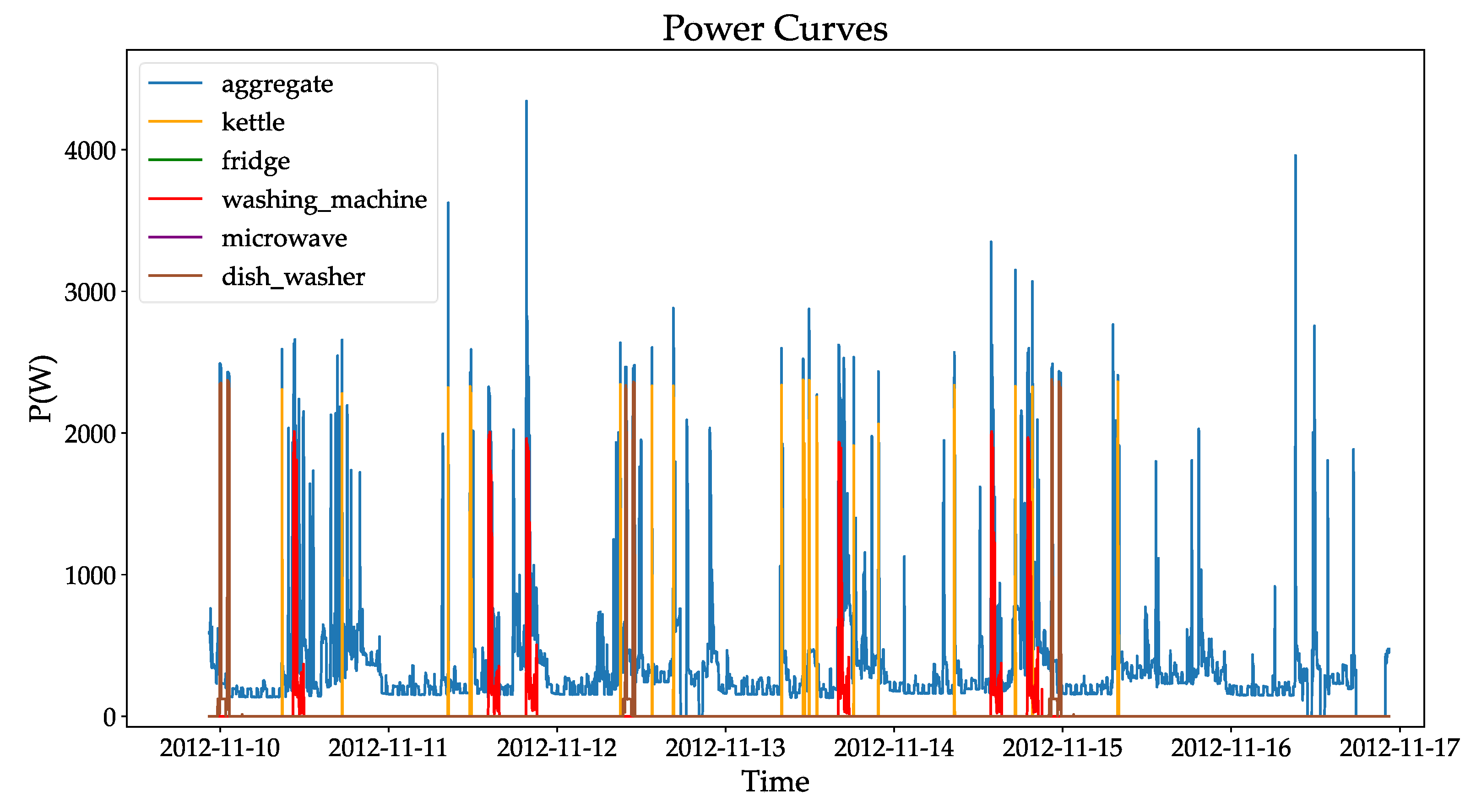
As shown in Figure 3 below, for a user within 7 days of the total power consumed by household electrical appliances and the power consumed by each electrical appliance individually, the total power is superimposed by the power consumed by each individual electrical appliance. The essence of the NILM algorithm is actually based on the identification of different loads during steady state operation or the switching operating state when the different electrical features can be classified into steady state features and transient features, which are also divided into non-traditional features in [15,22]. The commonly used load feature library classification and feature extraction methods are shown in Table 1 below.
Compared with transient features, steady state features are the most commonly used feature variables in NILM. This is due to the fact that most transient features occur at the moment the load state changes and during load switching, which requires a high-frequency sampling device to capture the state at the moment the transient feature occurs. Although high-frequency sampling devices can capture a range of load information, they are expensive, have a large amount of data, and require the use of high-performance computing equipment, which results in increased user costs and a long computing time. Therefore, it is more appropriate to set up a load information acquisition device in the home environment to extract the steady state characteristics of the load.
2.1.1. Homeostatic Characteristics
The characteristics of the current, active power, and reactive power in steady-state operation are different for different electrical appliances. Figure 4 below shows the current, active power, and reactive power waveforms of a laptop computer, a water dispenser, a microwave oven, and a laser printer in a user’s home during steady-state operation.
From the four sets of waveforms shown in Figure 4, it can be seen intuitively that different loads have their own unique current and active/reactive power characteristics. The current characteristics can be symbolized by the mean , the root-mean-square , and the maximum values of the current , which are quantified by the following equations:
where is the duration of the state.
With the broad application of deep learning algorithms in the field of image processing in recent years, ref. [23] proposed that the V-I trajectory characteristics of the load, in combination with a convolutional neural network, be used to weight-pixelize the V-I trajectory map as the input of the network. In addition, in order to extract more load information from the V-I trajectories, ref. [24] color-coded the V-I trajectory images to maximize the classification ability of the images and transform the V-I trajectories into visual features. The authors of [25] proposed a machine learning algorithm using semi-supervised learning to solve the problem of the inability of a load operating state that has diverse V-I trajectories to correctly identify the corresponding load. In this paper, we used the information on steady-state load collected by a home user’s acquisition device to extract the voltage and current data over one cycle corresponding to four types of electrical equipment in order to plot the V-I trajectory.
When plotting the V-I curve, in order to avoid the influence of the differences in the amplitude of the voltage and current during the steady-state operation of different pieces of electrical equipment, we unified the voltage and current data for data preprocessing. The two parameters were normalized to values between 0 and 1 to reduce the influence of the different magnitudes of the two parameters. The normalized formula is as follows:
After processing the voltage–current data using Equation (6), we plotted the V-I curve, which is shown in Figure 5 below.
From the V-I trajectories of the four electrical appliances shown in Figure 5 above, it can be seen that different electrical appliances have different V-I trajectory characteristics, and each V-I trajectory map contains different characteristic information for the identification of electrical appliances. When using V-I trajectories for NILM, the main concern is the information on stress, such as the curvature, total area, asymmetry, and slope of the V-I trajectories. The formula for the slope of the curve is as follows
where denotes the voltage span, denotes the current span, denotes device , and denotes the state circumference of the device.
2.1.2. Transient Characteristics
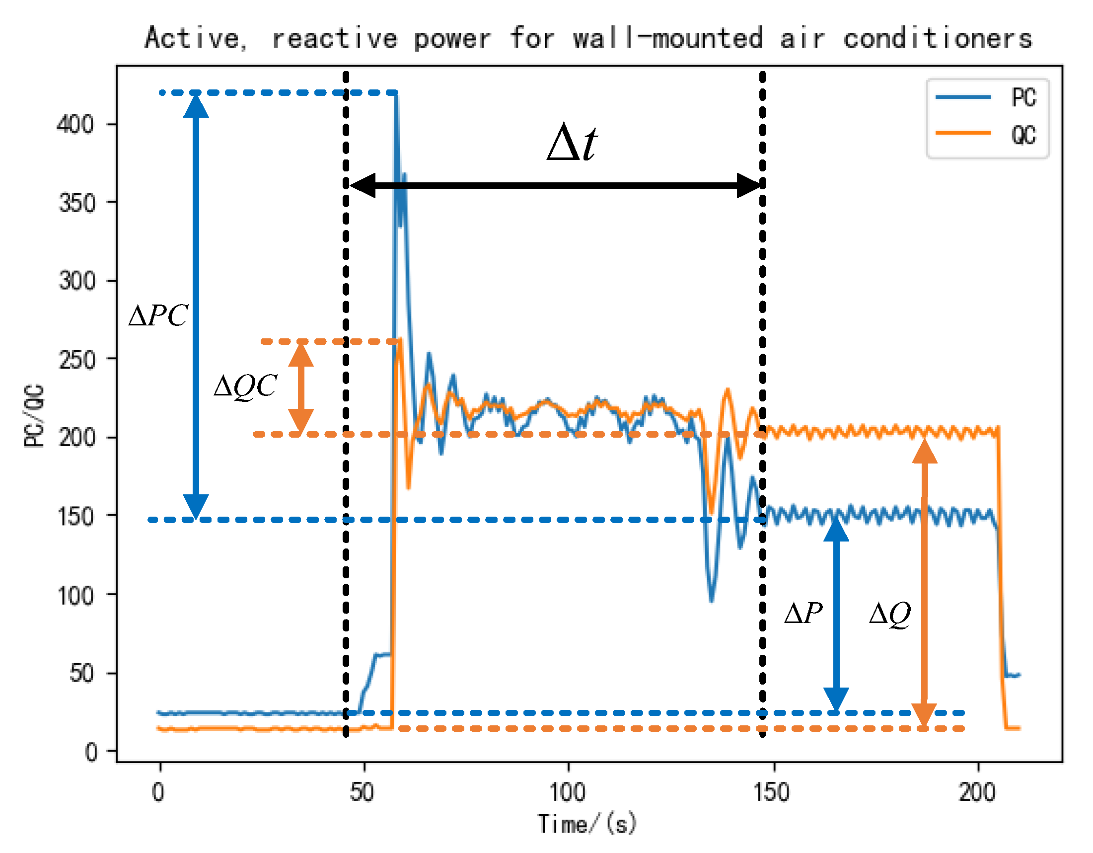
During the transition of electrical equipment from one state to another, such as from startup to stable operation or from stable operation to shutdown, there is a short period of switching known as the transient characteristics. These characteristics require a high sampling frequency for the sampling device due to the quick nature of the transient process. The NILM algorithm aims to improve the load identification accuracy by considering both steady state and transient load characteristics. For instance, ref. [26] suggests that the load data be pre-screened using the time and power jump values of the transient process between two state jumps. This method uses a support vector machine (SVM) to identify the load. The commonly used transient features include the transient transition time, inrush power multiplier, and active/reactive power jump values. These are shown in Figure 6 below, which illustrates the transition process of electrical equipment from startup to steady state.
The time required for an electrical device to transition from its current state to the next state is represented by the transient transition time . The formula for this is expressed as follows:
The active power jump variable represents the difference between the active power of the load in the previous steady state and the active power when it reaches the new steady state after passing through the transient process, which is expressed by the following formula:
The reactive power jump variable represents the difference between the reactive power of the load at the previous steady state and the reactive power when the load reaches the new steady state after passing through the transient process, which is expressed by the following formula:
The impact power multiplier indicates the relationship between the peak value reached by the power of the electrical equipment in the transient process and the power when it reaches the next steady state, which is expressed by the following formula:
The difference between the peak active power in the transient state and the active power after the transient state is denoted . The difference between the peak reactive power and the reactive power after the transient state is denoted . The formula is expressed as follows:
2.2. Dataset
Regardless of whether the steady state or transient characteristics of loads are chosen, the implementation of NILM must rely on household load data acquired in real scenarios. In recent years, with the growing interest in load identification, there has been a gradual increase in NILM-related datasets, and there are already many high-quality datasets available for researchers in this field [27,28]. We introduce several commonly used datasets below.
The UK-DALE dataset [29], provided by Jack Kelly in the UK, offers information on the electrical energy consumption of all electrical equipment in the homes of five householders over a period of time. The data were recorded every 6 s by a collection device for each household. To provide data with richer high-frequency load information, the voltage and current of the entire house were recorded at 16 kHz for three of the five households. Additionally, the dataset includes energy consumption data for one home over a period of 655 days. The REDD dataset, provided by Kolter and Johnson in the U.S. [30], offers both high-frequency and low-frequency data. The low-frequency data contain information on six households. The collection device recorded energy consumption data for each electrical device in each household, as well as the overall energy consumption data, at a sampling rate of 1 Hz. The high-frequency data were sampled at 15 kHz, and load energy data were collected for two households. Anderson et al. [31] provided the BLUED dataset, which includes the electricity usage and state transition information on each electrical device in a U.S. household for one week at a sampling frequency of 12 kHz.
These datasets are commonly used to validate NILM algorithms. The UK-DALE dataset is preferred due to its rich information, the appropriate amount of user data captured, and the length of time compared with the other two datasets. In this study, we used the UK-DALE data to divide the training and validation samples. We validated the non-intrusive load decomposition model with the parallel multiscale attention mechanism proposed in this paper. In order to facilitate subsequent cross-household experiments with the model, we selected electrical devices owned by both Household User 1 and Household User 2 in the UK-DALE dataset. In this study, washing machines, dishwashers, and refrigerators were selected as target loads. The total power and the power curves of the three types of electrical appliances for Household User 1 and Household User 2 in one day are shown in Figure 7 below.
As can be seen in Figure 7, the power curves of the refrigerator and dishwasher are simpler, with only two states (on and off) present during the operation of the appliance. However, the power curve of the washing machine [32] has multiple load fluctuation patterns, meaning there are switching operating states. For Household User 1, the maximum power of the refrigerator is 253.78 W, the maximum power of the dishwasher is 2419.01 W, and the maximum power of the washing machine is 2004.73 W. For Household User 2, the maximum power of the refrigerator is 102.58 W, the maximum power of the dishwasher is 2041.4 W, and the maximum power of the washing machine is 2242.19 W.
3. Smart Home Modeling Using Non-Intrusive Load Decomposition
3.1. Model Structure
The smart home model based on non-intrusive recognition designed in this study consists of a decision control part, an execution control part, and an information perception part. The overall model framework is shown in Figure 8.
The execution control part contains most of the electrical devices used within the home, and the user can expand the entire system by increasing the size of the lower computer module. The upper computer module communicates with each lower computer module using Zigbee technology in order to reduce the layout difficulties caused by the line connection. The information perception part consists of two subparts: the traditional collection module and the information collection device, which is dedicated to non-invasive load recognition. The model monitors the environmental conditions in the home in real time by means of traditional collection modules, such as temperature detection sensors, humidity detection sensors, and smoke concentration detection sensors, and the monitored data are summarized and sent to the decision-making control part. The non-intrusive load recognition model adopts a special voltage and current collection device, with a set sampling frequency of 1/6 Hz, and puts the data collected on power consumption into the parallel multiscale information collection device proposed in this paper. In the proposed load decomposition model with the parallel multiscale attention mechanism, the energy consumption data used by the corresponding electrical equipment over a period of time are extracted. The decision control part sends control commands to the executive control part using the data transmitted from the information perception part. It then summarizes the data and provides to the user through the visualization interface specific information on the home environment and electrical equipment.
3.2. A Non-Intrusive Load Decomposition Model Based on a Parallel Multiscale Attention Mechanism
Non-intrusive load identification is a typical time series problem that aims to decompose the energy consumed by individual electrical devices from the total power consumption. Equation (1) shows that the total power consumption of household loads at a certain moment is not only determined by the power of all operating devices at that moment but also by the operating status of the devices at that moment. Commonly used methods for solving time series problems include the sequence-to-sequence model (Seq2Seq), the Long Short-Term Memory (LSTM) recurrent neural network, and the convolutional neural network (CNN). In this study, we used a sequence-to-point (Seq2Point) learning model, which has shown a greater ability to decompose the load compared with the Seq2Seq model, while also requiring less computation time [33]. In this paper, we present a non-intrusive load decomposition model that incorporates a parallel multiscale attention mechanism (PMAM) based on the existing model.
3.2.1. Sequence-to-Point Learning Model
The sequence-to-point (Seq2Point) learning model maps the input time series data to the output sequence. Unlike the Seq2Seq model, the output of the Seq2Point model becomes a single prediction for each midpoint element of the target device, rather than an average of the predicted data across the entire output window, which helps to reduce the amount of time required to train the model and produces more accurate predictions.
After the raw total power data are input into the Seq2Point model, after encoding the raw data, the model maps the input total power data in the sliding window fragments to the corresponding output window at the midpoint . The mapping relation function can be expressed by Equation (14):
where denotes a sliding time window of length starting from and denotes random Gaussian noise. In order to make the predicted value of the model close to the true value, the loss function of the model can be defined as:
where is the parameter of the training network.
In the learning model of the sequence problem, in order to ensure that the acquired input sequence features contain rich feature information rather than focus too much on a single representation, we adopted a parallel multiscale attention mechanism to simultaneously learn the contextual representation information at different scales and combined the self-attention mechanism with a convolution to learn the sequence at different scales.
3.2.2. Parallel Multiscale Attention Mechanism
The self-attention mechanism has a huge advantage when using local information. When faced with information containing multiple features, it can selectively focus on a certain feature while ignoring the other features, and it can simulate very long dependency relationships. In order to obtain both local and global feature information, we adopted a parallel multi-channel attention mechanism, the structure of which is shown in Figure 9.
As the collected load information is characterized by high dimensionality, redundant information, and a large amount of information, we pooled the data in order to simplify the complexity of the network. Pooling not only expands the perception of information but also has invariance. The characteristics of the data, such as translation, rotation, and scale, do not change after pooling, which both speeds up the calculation and prevents overfitting. Maximum pooling is one of the most-adopted pooling methods and is able to select the largest value in each pooling window as the output in order to achieve feature reduction and extraction. In performing non-invasive load decomposition, in addition to focusing on the most significant features, it is also necessary to focus on the overall data features. For this reason, we adopted both maximum pooling and average pooling. The most significant data features were obtained through maximum pooling, and the overall data features were obtained through average pooling. The two datasets were fused into the input of the next level of the parallel multiscale attention mechanism.
The parallel multiscale attention mechanism is the key part of the non-invasive decomposition model, which has three main parts: the self-attention mechanism that can capture the global feature information, the depth-separable convolution that acquires the local feature information, and the position feed-forward network that captures the labeled features [34]. The relationship between the output of the model and the output can be expressed as follows:
where denotes the sequence data input into the layer, denotes the self-attention mechanism function, denotes the depth-separable convolution function, and denotes the position feed-forward network function.
In the self-attentive mechanism function, the input sequence , is first linearly transformed to obtain the desired Query (), Key (), and Value () variables. The linear transformation is shown in Equation (17):
Secondly, the attention score is obtained after calculating the similarity of and . The obtained attention score is normalized to a probability distribution using the function. Finally, the final attention value is obtained by a weighted summation with based on the normalized result. The calculation formula is shown in Equation (18):
where denotes the variance in the normalized probability distribution. Since the distribution of the probability distribution obtained by the function is related to the variance , the probability distribution obtained by the function needs to be decoupled from the variance during the computation to ensure that the gradient value of the model remains stable during the training process.
In contrast to the conventional convolution operation, the depth-separable convolution used in this paper employs a convolution kernel that is responsible for only one channel, rather than multiple channels. As a result, the number of convolution kernels and the number of channels in the previous layer are the same, and each channel is calculated independently of the others. We utilized a position feed-forward network in conjunction with the depth-separable convolution to provide richer feature information for the model. This approach addresses the issue of the model’s inability to fully explore the feature information at the same spatial location.
3.2.3. Feature Extraction Networks
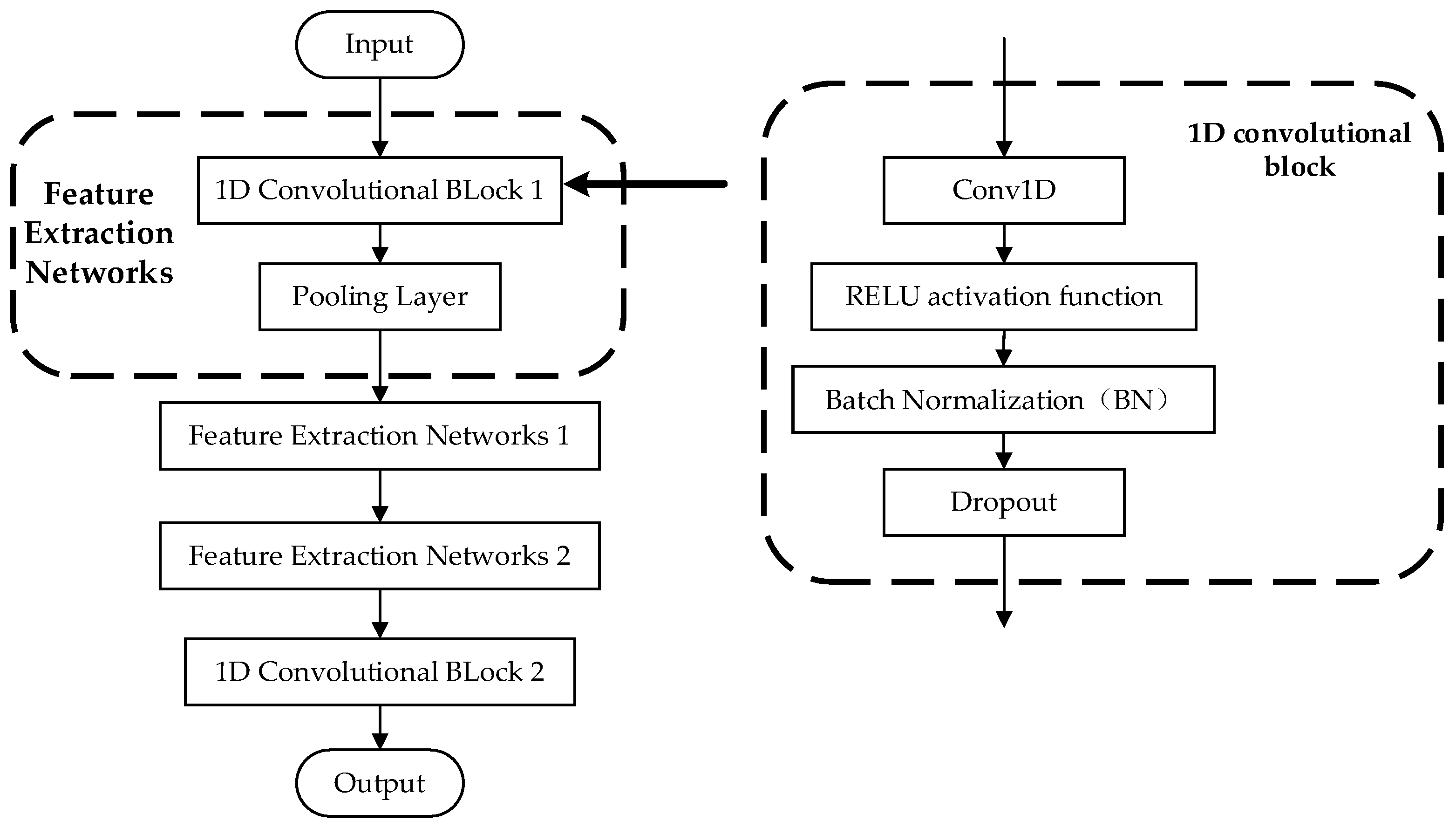
The feature extraction network aims to filter the input long-term sequence data and remove redundant information to obtain the important features of the sequence data. The PMAM decomposition model’s input layer employs four sets of one-dimensional convolutional blocks and pooling layers to form the feature extraction network. The one-dimensional convolutional block has four components: a one-dimensional convolution (Conv1D), a RELU activation function, batch normalization (BN), and Dropout. Figure 10 provides a visual representation.
In the feature extraction network, the local features of sequence data are extracted by multiple 1D convolutional blocks, and, as the layers of 1D convolutions are further stacked, more and more feature information can be captured, which improves the ability of the model to globally sense the input long-term sequence data [35]. The decomposition performance of the PMAM model is also affected by the hyperparameters, such as the number of convolution kernels in the 1D convolutional block, the convolution kernel’s dimensions, and the activation function settings. The model’s decomposition effect varies depending on the hyperparameter settings [36]. In this study, the PMAM model used four groups of 1D convolutional blocks for feature extraction. Each group had a different number of convolutional kernels (32, 61, 128, and 320). Additionally, the number of feature channels in each group of convolutional blocks was increased from 1 to 128.
The one-dimensional convolutional block uses the Rectified Linear Unit (RELU) as its activation function to improve the nonlinear relationship between the layers in the network. The RELU activation function is effective in solving the problem of gradient vanishing in non-negative intervals due to its constant gradient. Additionally, it sparsifies the network by resulting in some outputs being 0. This allows the model to better identify relevant features and fit the training data.
3.2.4. Parallel Multiscale Feature Fusion
In a fixed deep learning network architecture, the network’s learning scale is typically unchangeable and challenging to adjust to the task objectives. This limitation restricts the model to only obtaining information on a fixed scale during the learning process. To enable the model to learn multiscale information, we propose a multiscale network architecture.
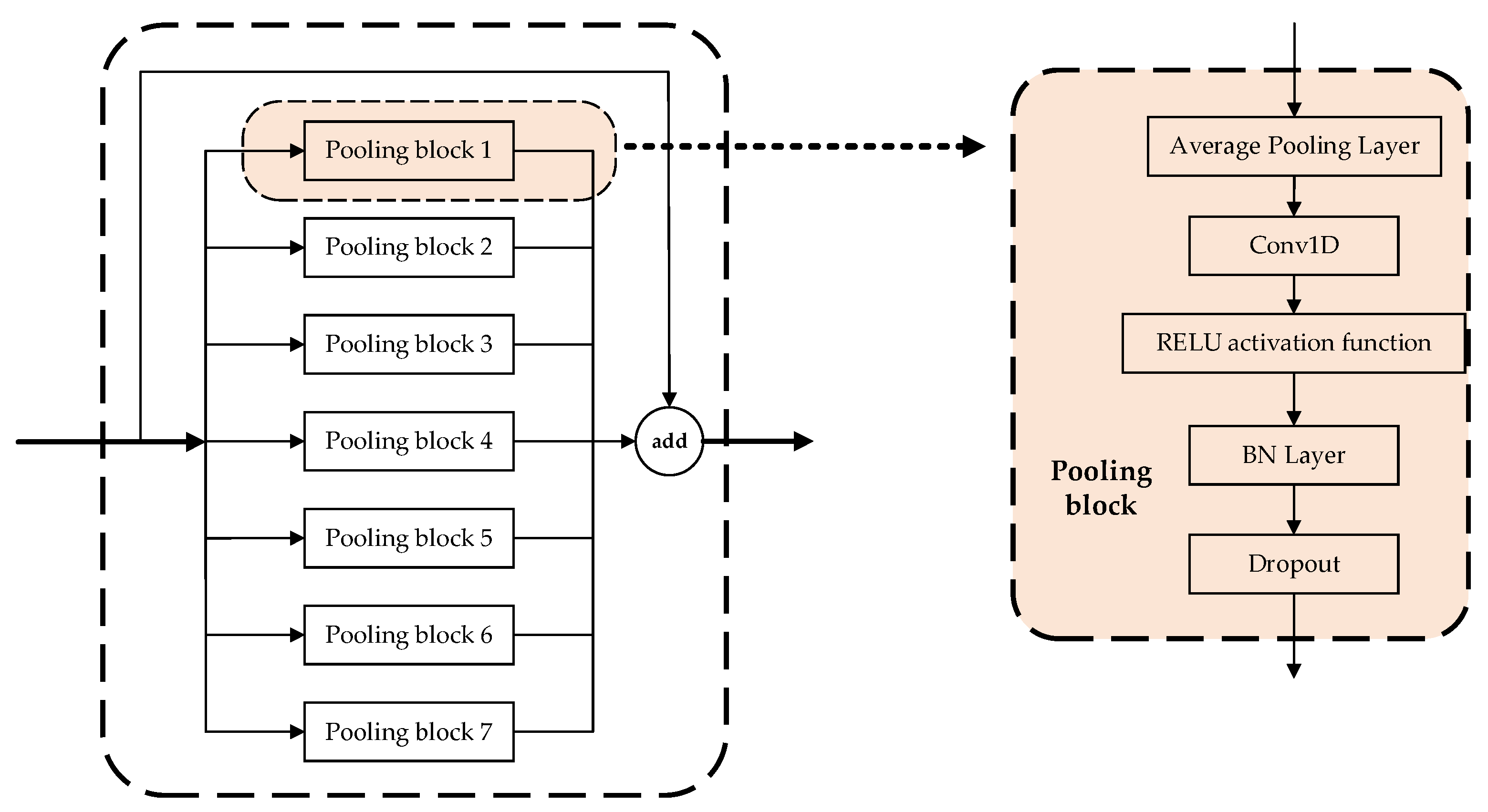
Two frequently used multiscale network structures are serial networks and parallel multibranch networks [37]. Serial networks use layer-hopping connections to combine different scale features, while parallel multibranch networks use various convolutional kernels with different sizes, null convolutions, and pooling to obtain feature information on different scales within the same layer. Finally, they pass the feature fusion on to the next layer. In comparison with serial networks, parallel networks can significantly enhance the model’s computational ability and reduce the required computing time. Therefore, we employed a parallel multiscale network in the temporary pooling layer of the PMAM model to merge the load features at seven different scales, as illustrated in Figure 11 below.
In a parallel multiscale network, each pooling block has five components: an average pooling layer, a 1D convolution, the RELU activation function, a BN layer, and Dropout. The input data for feature information in the parallel multiscale network are transformed into load features of varying sizes through the average pooling layer in different pooling blocks. Subsequently, the size of the output load feature is made consistent by using 1D convolution. The size of the convolution kernel used for 1D convolution is 64. The feature information from the seven sets of pooling blocks is combined with the feature information inputted into the parallel multiscale network to obtain the final load feature. The seven pooled blocks are then fused with the input data of the parallel multiscale network to obtain the final load features.
3.3. Model Parameter Selection
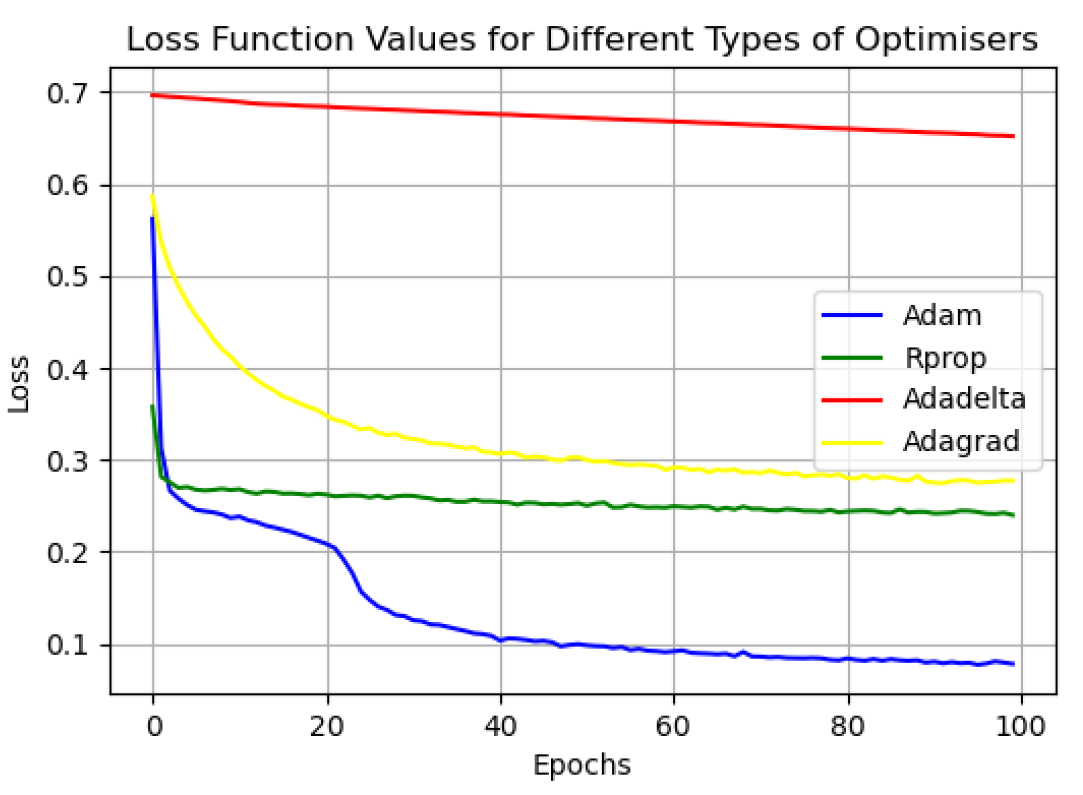
In the model parameter settings, we set the number of data samples (Batchsize) used in a single pass to train the model to 1470, and we set the number of times the model was trained to 100. As overfitting may occur during the model training process, we used the optimizer to manage and update the values of the learnable parameters in the model, which is conducive to a closer match between the training results of the model and the real values. Figure 12 shows the results of the loss values of the model training by the different optimizers used in this study.
As can be seen in Figure 12, the Adam optimizer is able to converge quickly and stabilize the loss values of the model compared with the other optimizers when the model is trained. For example, the Adadelta optimizer does not converge even after being trained 100 times, and the convergence performance is not good. Therefore, in this study, the Adam optimizer was used to train the model. In order to verify the convergence performance of the Adam optimizer on the model at different learning rates, we tested the loss value of the model during training at learning rates of 0.0001, 0.001, 0.005, and 0.01. The test results are shown in Figure 13 below, according to which it can be found that the model is better trained at a learning rate of 0.005.
4. Algorithm Analysis
4.1. Hardware and Software Platform
This study’s hardware environment consisted of a 64-bit computer with an Intel(R) Core(TM) i7-11800H @ 2.30 GHz processor and 16.0 GB of RAM. The software platform used was the Windows 10 Professional operating system, Python 3.7.4, and the Tensorflow-gpu version 2.1 deep learning framework. The model structure shown in Figure 8 was used to train the UK-DALE data.
4.2. Load Decomposition Evaluation Metrics
To assess the performance of the training model, we used several evaluation metrics, including the F1 score, precision rate, recall rate, accuracy rate, Matthews correlation coefficient (MCC), and mean absolute error (MAE). Among them, the confusion matrix is the most commonly used performance evaluation matrix in the field of machine learning, and we calculated the required evaluation indexes, such as the F1 score, precision rate, and recall rate, according to the results of the confusion matrix. The structure of the confusion matrix is shown in Figure 14.
In the confusion matrix, means that the result of the model decomposition is consistent with the actual working state of the electrical equipment, Positive means that the electrical equipment is in the working state, and means that the electrical equipment is in the non-working state. The formulas for Precision, Accuracy, Recall, F1 score, and MCC are as follows:
MAE denotes the mean absolute value of the difference between the model’s predicted value and the true value over a period of time and is expressed in the following equation:
4.3. Experimental Results and Analysis
In conducting experiments on the PMAM load decomposition model, the experimental process was divided into data collection, hyperparameter setting, model training, and model evaluation. For this study, we selected the total power data on Household User 1 and the electrical data on each electrical device from the publicly available UK-DALE dataset, covering the period from April 2013 to December 2014. The collected data have been preprocessed. The model was trained using the preprocessed data and the set hyperparameters. Subsequently, the load decomposition effect of the PMAM model was verified using each load decomposition evaluation index proposed in Section 4.2. The experimental flow is illustrated in Figure 15.
In this study, the data on dishwasher and washing machine loads and the corresponding operating states in the UK-DALE data were selected. After we applied the PMAM load decomposition model proposed in this paper, the decomposition results of their operating states were compared with the real operating states of the electrical equipment as shown in Figure 16 below.
From the work state prediction results shown in Figure 16, it can be seen that the model has a good load decomposition ability and can more accurately achieve the extraction of the target load work state from the bus data containing the work state of multiple devices. In order to better validate the performance of this model, we used the electrical appliance data on Household User 1 from the same UK-DALE dataset to train the Long Short-Term Memory (LSTM) recurrent neural network model, the Time Pooling-Based Load Disaggregation Model (TPNILM) [38], the Extreme Learning Machine (ELM) [39], and the same network structure as in this paper, but without the parallel multi-scalar attention mechanism. The training set for Household User 1 consisted of data from a specific period of time, while the data used to train the model were taken from a different period than that of the test. After the model training was completed, we obtained the performance evaluation index of each model, which is shown in Table 2 below.
As can be seen from Table 2, the PMAM model proposed in this paper outperforms the other four decomposition models in most of the load decomposition performance metrics. The F1 scores of the PMAM model for decomposing the three types of loads, namely dishwasher, washing machine, and refrigerator loads, remain above 0.9 and are better than those of the other load decomposition models. The F1 scores were also improved by an average of 8.5 percent compared with those of the ELM model, which showed a good ability to decompose the loads. The PMAM model is optimal in the recall evaluation index for all types of electrical equipment except for dishwashers, where its performance is slightly lower than that of the ELM model. The PMAM model also improves the recall by 3% compared with the TPNILM model. Although the ELM model performs the best in the MAE decomposition performance index, the PMAM model proposed in this paper outperforms the other models in terms of overall decomposition performance. Under the same network, compared with the Load Disaggregation Model without Parallel Multi-scalar Attention Mechanisms (UNPMAM), the average absolute errors of both appliances were reduced, and they were also slightly better than the UNPMAM in terms of the F1 score.
Compared with the F1 evaluation metrics of the UNPMAM in the washing machine, the F1 metrics of the PMAM model proposed in this paper are significantly better than those of the UNPMAM in both the dishwasher and the refrigerator. The power of the washing machine fluctuates greatly during operation and its working state transitions frequently, as shown in Figure 7. In contrast, the refrigerator has a clear periodicity during operation, and the power required for each cycle is relatively stable with distinct load characteristics. It is important to note these differences in power consumption between the two appliances. Table 2 shows that all models have a significant deviation from the actual washing machine decomposition results. Additionally, Household User 1 uses the washing machine less frequently, resulting in a smaller number of required training samples. As a result, the PMAM model cannot effectively extract the load characteristics. Therefore, to enhance the model’s ability to extract deep load features, further research will be conducted to extract the load features of electrical appliances that frequently switch operating states. Additionally, the super-parameters of the feature extraction network will be optimized.
In order to validate the generalizability of the PMAM model proposed in this paper, data from Household User 2 in the UK-DALE dataset were selected for cross-household experiments. The model’s training set was selected from Household User 1’s data between April 2013 and December 2014, while the test set was selected from Household User 2’s data for a one-month period in order to conduct load decomposition tests. The results of the tests are presented in Table 3 below.
Table 3 shows that the PMAM model maintains good decomposition performance even when tested with data from untrained Household User 2. The model outperforms the other models in most performance evaluation metrics. In the performance evaluation index of the PMAM model’s decomposition of the refrigerator data, the model’s MAE is the lowest. Although the F1 score of the ELM model is higher than that of the PMAM model, the difference is only 1.6%. However, the MAE of the PMAM model is 31% lower than that of the ELM model. Therefore, it appears that the PMAM model proposed in this paper is superior overall. In the performance evaluation of the PMAM model on the washing machine data, the PMAM model outperforms the other models with higher F1 scores (an 11% increase compared with the TPNILM model). The results in Table 2 and Table 3 demonstrate the superior generality of the PMAM model proposed in this paper.
When implementing smart grid technology, it is important to consider the model’s generalization and load decomposition capabilities as well as its training time and computational requirements. To achieve this, we compared the number of model parameters and the training time required by different models, as shown in Table 4.
From Table 4, it can be seen that the PMAM model requires more computations compared with the other models, which is due to the fact that the PMAM model uses a parallel multiscale feature fusion network, which captures both global and local features through a parallel multiscale attention mechanism, resulting in an increase in the number of model parameters. Compared with the other models, the PMAM model proposed in this paper has a smaller difference in the training time per epoch. It also has a comprehensive decomposition capability that can still be applied to NILM. However, there is still room to optimize the number of computations that the model requires when deployed in real smart grid projects. The complexity of the model can be optimized while maintaining the decomposition performance.
5. Conclusions
This paper presented a non-intrusive load decomposition model with a parallel multiscale attention mechanism that combines non-intrusive load identification technology with smart home technology to improve the energy demand-side response under the development of smart grids and new power systems. Incorporating the multiscale attention mechanism in the training network captures both global and local feature information, expanding the perceptual field of the model. Additionally, the model’s decomposition performance is improved to a certain extent by the multiscale feature fusion network. After validating the PMAM model with two household users from the UK-DALE dataset, we proposed a model with better generalizability and improved accuracy and F1 score values compared with the other models. The experimental results indicate that the PMAM model maintains F1 scores above 0.9 for refrigerator, dishwasher, and washing machine data under the same household user. On average, the F1 scores improved by 2.1% and the MAE decreased by 6.84% compared with the UNPMAM. This suggests that the model’s decomposition performance was better after the parallel multiscale attention mechanism was added. In the cross-family test, the PMAM model demonstrated a superior decomposition ability, maintaining an F1 score above 0.85. On average, compared with the other models, the F1 score increased by 15.34%, indicating better generalizability. The PMAM model allows for the decomposition of data on household electrical equipment, providing users with a clear understanding of the working status of each device in the household. Users can utilize the information on the operational status of their loads to establish a home energy management system. This system can optimize the scheduling of household electrical equipment, resulting in reduced energy loss and cost savings while maintaining user comfort.
In future research, the PMAM model’s decomposition results will be combined with a home energy management system to optimize equipment scheduling by considering the working status of each electrical device. Additionally, depending on the energy suppliers’ buying and selling policies, home users with energy storage devices or electric vehicles can achieve better energy returns. Simultaneously, information on electrical equipment obtained from decomposition can be linked to the user’s behavior, allowing for the prediction of the user’s next action based on their use of a particular electrical device. This may enhance the intelligence of household equipment and improve the user’s experience.
Author Contributions
Conceptualization and methodology, J.W.; software and validation, J.W.; formal analysis and investigation, J.W.; data curation and writing—original draft preparation, J.W.; writing—review and editing, C.Z.; visualization and supervision, L.Y. All authors have read and agreed to the published version of the manuscript.
Funding
This research was funded by the National Natural Science Foundation of China (No. 51707121).
Data Availability Statement
The original contributions presented in the study are included in the article, further inquiries can be directed to the corresponding author.
Conflicts of Interest
The authors declare no conflicts of interest.
References
- Lu, J.; Zhao, R.; Liu, B.; Yu, Z.; Zhang, J.; Xu, Z. An Overview of Non-Intrusive Load Monitoring Based on VI Trajectory Signature. Energies 2023, 16, 939. [Google Scholar] [CrossRef]
- Aboulian, A.; Green, D.H.; Switzer, J.F.; Kane, T.J.; Bredariol, G.V.; Lindahl, P.; Donnal, J.S.; Leeb, S.B. NILM dashboard: A power system monitor for electromechanical equipment diagnostics. IEEE Trans. Ind. Inform. 2018, 15, 1405–1414. [Google Scholar] [CrossRef]
- Li, J.; Xu, W.; Zhang, X.; Feng, X.; Chen, Z.; Qiao, B.; Xue, H. Control method of multi-energy system based on layered control architecture. Energy Build. 2022, 261, 111963. [Google Scholar] [CrossRef]
- Koseleva, N.; Ropaite, G. Big data in building energy efficiency: Understanding of big data and main challenges. Procedia Eng. 2017, 172, 544–549. [Google Scholar] [CrossRef]
- He, X.; Dong, H.; Yang, W.; Hong, J. A Novel Denoising Auto-Encoder-Based Approach for Non-Intrusive Residential Load Monitoring. Energies 2022, 15, 2290. [Google Scholar] [CrossRef]
- Gopinath, R.; Kumar, M.; Joshua, C.P.C.; Srinivas, K. nergy management using non-intrusive load monitoring techniques—State-of-the-art and future research directions. Sustain. Cities Soc. 2020, 62, 102411. [Google Scholar] [CrossRef]
- Armel, K.C.; Gupta, A.; Shrimali, G.; Albert, A. Is disaggregation the holy grail of energy efficiency? The case of electricity. Energy Policy 2013, 52, 213–234. [Google Scholar] [CrossRef]
- Desley, V.; Laurie, B.; Peter, M. The effectiveness of energy feedback for conservation and peak demand: A literature review. Open J. Energy Effic. 2013, 2013, 28957. [Google Scholar]
- Bonfigli, R.; Principi, E.; Fagiani, M.; Severini, M.; Squartini, S.; Piazza, F. Non-intrusive load monitoring by using active and reactive power in additive Factorial Hidden Markov Models. Appl. Energy 2017, 208, 1590–1607. [Google Scholar] [CrossRef]
- Qu, L. Research and Application of Non-Intrusive Load Monitoring Technology Based on Event Detection. Ph.D. Thesis, Hangzhou University of Electronic Science and Technology, Hangzhou, China, 2023. [Google Scholar]
- Hart, G.W. Prototype Nonintrusive Appliance Load Monitor; Technical Report 2; MIT Energy Laboratory and Electric Power Research Institute: Concorde, MA, USA, 1985. [Google Scholar]
- Hart, G.W. Nonintrusive appliance load monitoring. Proc. IEEE 1992, 80, 1870–1891. [Google Scholar] [CrossRef]
- Xu, X.H.; Zhao, S.T.; Cui, K.B. A non-intrusive load decomposition algorithm based on convolutional block attention model. Grid Technol. 2021, 45, 3700–3706. [Google Scholar]
- Kelly, J.; Knottenbelt, W. Neural nilm: Deep neural networks applied to energy disaggregation. In Proceedings of the 2nd ACM International Conference on Embedded Systems for Energy-Efficient Built Environments, New York, NY, USA, 4–5 November 2015; pp. 55–64. [Google Scholar]
- Batra, N.; Singh, A.; Whitehouse, K. Neighbourhood nilm: A big-data approach to household energy disaggregation. arXiv 2015, arXiv:1511.02900. [Google Scholar]
- Nalmpantis, C.; Vrakas, D. Machine learning approaches for non-intrusive load monitoring: From qualitative to quantitative comparation. Artif. Intell. Rev. 2019, 52, 217–243. [Google Scholar] [CrossRef]
- Yang, F.; Liu, B.; Luan, W.; Zhao, B.; Liu, Z.; Xiao, X.; Zhang, R. FHMM based industrial load disaggregation. In Proceedings of the 2021 6th Asia Conference on Power and Electrical Engineering (ACPEE), Chongqing, China, 8–11 April 2021; pp. 330–334. [Google Scholar]
- Jiao, X.; Chen, G.; Liu, J. A non-intrusive load monitoring model based on graph neural networks. In Proceedings of the 2023 IEEE 2nd International Conference on Electrical Engineering, Big Data and Algorithms (EEBDA), Changchun, China, 24–26 February 2023; pp. 245–250. [Google Scholar]
- Kang, J.S.; Yu, M.; Lu, L.; Wang, B.; Bao, Z. Adaptive non-intrusive load monitoring based on feature fusion. IEEE Sens. J. 2022, 22, 6985–6994. [Google Scholar] [CrossRef]
- Gao, Y.; Yang, H. Domestic load identification based on transient feature closeness matching. Power Syst. Autom. 2013, 37, 54–59. [Google Scholar]
- Wang, K.; Zhong, H.; Yu, N.; Xia, Q. Non-intrusive load decomposition for residential users based on seq2seq and Attention mechanism. Chin. J. Electr. Eng. 2019, 39, 75–83+322. [Google Scholar]
- Shi, Y.T. Research and Application of Non-Intrusive Load Identification Method Based on Deep Learning. Ph.D. Thesis, Hangzhou University of Electronic Science and Technology, Hangzhou, China, 2023. [Google Scholar]
- De Baets, L.; Ruyssinck, J.; Develder, C.; Dhaene, T.; Deschrijver, D. Appliance classification using VI trajectories and convolutional neural networks. Energy Build. 2018, 158, 32–36. [Google Scholar] [CrossRef]
- Wang, S.; Chen, H.; Guo, L.; Xu, D. Non-intrusive load identification based on the improved voltage-current trajectory with discrete color encoding background and deep-forest classifier. Energy Build. 2021, 244, 111043. [Google Scholar] [CrossRef]
- Han, Y.; Li, K.; Feng, H.; Zhao, Q. Non-intrusive load monitoring based on semi-supervised smooth teacher graph learning with voltage–current trajectory. Neural Comput. Appl. 2022, 34, 19147–19160. [Google Scholar] [CrossRef]
- Mou, K.; Yang, H. A non-intrusive load monitoring method based on PLA-GDTW support vector machine. Grid Technol. 2019, 43, 4185–4193. [Google Scholar]
- Huber, P.; Ott, M.; Friedli, M.; Rumsch, A.; Paice, A. Residential power traces for five houses: The iHomeLab RAPT dataset. Data 2020, 5, 17. [Google Scholar] [CrossRef]
- Klemenjak, C.; Kovatsch, C.; Herold, M.; Elmenreich, W. A synthetic energy dataset for non-intrusive load monitoring in households. Sci. Data 2020, 7, 108. [Google Scholar] [CrossRef] [PubMed]
- Kelly, J.; Knottenbelt, W. The UK-DALE dataset, domestic appliance-level electricity demand and whole-house demand from five UK homes. Sci. Data 2015, 2, 150007. [Google Scholar] [CrossRef]
- Kolter, J.Z.; Johnson, M.J. REDD: A public data set for energy disaggregation research. In Proceedings of the Workshop on Data Mining Applications in Sustainability (SIGKDD), San Diego, CA, USA, 21–24 August 2011; Volume 25, pp. 59–62. [Google Scholar]
- Filip, A. Blued: A fully labeled public dataset for event-based nonintrusive load monitoring research. In Proceedings of the 2nd Workshop on Data Mining Applications in Sustainability (SustKDD), Beijing, China, 12–16 August 2012. [Google Scholar]
- Cui, P.F. Research on Non-Intrusive Household Electric Load Decomposition and Application Based on Deep Learning. Ph.D. Thesis, Xi’an University of Architecture and Technology, Xi’an, China, 2023. [Google Scholar]
- Zhang, C.; Zhong, M.; Wang, Z.; Goddard, N.; Sutton, C. Sequence-to-point learning with neural networks for non-intrusive load monitoring. In Proceedings of the AAAI Conference on Artificial Intelligence, New Orleans, LA, USA, 2–7 February 2018; Volume 32. [Google Scholar]
- Zhao, G.; Sun, X.; Xu, J.; Zhang, Z.; Luo, L. Muse: Parallel multi-scale attention for sequence to sequence learning. arXiv 2019, arXiv:1911.09483. [Google Scholar]
- Alhussein, M.; Aurangzeb, K.; Haider, S.I. Hybrid CNN-LSTM model for short-term individual household load forecasting. IEEE Access 2020, 8, 180544–180557. [Google Scholar] [CrossRef]
- Shao, X.; Kim, C.S.; Sontakke, P. Accurate deep model for electricity consumption forecasting using multi-channel and multi-scale feature fusion CNN–LSTM. Energies 2020, 13, 1881. [Google Scholar] [CrossRef]
- Xu, R.; Liu, D. Non-intrusive load monitoring based on multi-scale feature fusion and multi-head self-attention mechanism. Sci. Technol. Eng. 2024, 24, 2385–2395. [Google Scholar]
- Massidda, L.; Marrocu, M.; Manca, S. Non-intrusive load disaggregation by convolutional neural network and multilabel classification. Appl. Sci. 2020, 10, 1454. [Google Scholar] [CrossRef]
- Salerno, V.M.; Rabbeni, G. An extreme learning machine approach to effective energy disaggregation. Electronics 2018, 7, 235. [Google Scholar] [CrossRef]
Figure 1.
Smart grid architecture.

Figure 2.
Physical architecture of intrusive load detection and non-intrusive load detection.

Figure 3.
Power curve.

Figure 4.
(a) Laptop computer; (b) Water dispenser; (c) Microwave oven; (d) Laser printer. Current, active power, and reactive power waveforms during steady-state operation.
Figure 4.
(a) Laptop computer; (b) Water dispenser; (c) Microwave oven; (d) Laser printer. Current, active power, and reactive power waveforms during steady-state operation.


Figure 5.
V-I curves: (a) Laptop computer; (b) Water dispenser; (c) Microwave oven; (d) Laser printer.
Figure 5.
V-I curves: (a) Laptop computer; (b) Water dispenser; (c) Microwave oven; (d) Laser printer.

Figure 6.
Examples of transient characteristics.

Figure 7.
(a) Household User 1; (b) Household User 2. Total power and power curves for three types of electrical appliances.
Figure 7.
(a) Household User 1; (b) Household User 2. Total power and power curves for three types of electrical appliances.

Figure 8.
A framework for smart home modeling based on non-intrusive recognition.

Figure 9.
A non-intrusive decomposition model based on a parallel multi-channel attention mechanism.
Figure 9.
A non-intrusive decomposition model based on a parallel multi-channel attention mechanism.

Figure 10.
Structure of the feature extraction network.

Figure 11.
Parallel multiscale network structure.

Figure 12.
Model training loss values under different optimizers.

Figure 13.
Model training loss values at different learning rates.

Figure 14.
Confusion matrix structure.

Figure 15.
Experimental process.

Figure 16.
(a) dishwashers; (b) washing machine. Work status prediction results.


Table 1.
Commonly used load feature library classification and feature extraction methods.
| Feature Type | Specific Characteristics | Feature Extraction Method |
|---|---|---|
| Homeostatic Characteristics | voltage/current characteristics | statistical analysis |
| active/reactive power characteristics | statistical analysis | |
| harmonic characteristic | Fast Fourier Transform (FFT) | |
| peripheral V-I characteristics | relevant indicators used to characterize trajectories | |
| Transient Characteristics | prompt power | power spectral envelope estimation, waveform vectors |
| instantaneous current | Fast Fourier Transform (FFT) | |
| voltage noise | spectral analysis |
Table 2.
Comparison of the load-splitting performance evaluation metrics for Household User 1.
| Electrical Equipment | Modeling | Evaluation Indicators | |||||
|---|---|---|---|---|---|---|---|
| F1 | Precision | Recall | Accuracy | MAE | MCC | ||
| Dishwasher | PMAM | 0.966 | 0.967 | 0.965 | 0.998 | 20.44 | 0.965 |
| UNPMAM | 0.933 | 0.908 | 0.959 | 0.997 | 21.37 | 0.932 | |
| LSTM | 0.06 | 0.03 | 0.63 | 0.35 | 130 | - | |
| TPNILM | 0.930 | 0.942 | 0.919 | 0.997 | 20.41 | 0.928 | |
| ELM | 0.93 | 0.89 | 0.99 | 0.98 | 19 | - | |
| Washing machine | PMAM | 0.989 | 0.987 | 0.991 | 0.998 | 41.48 | 0.988 |
| UNPMAM | 0.984 | 0.985 | 0.982 | 0.998 | 41.51 | 0.982 | |
| LSTM | 0.09 | 0.05 | 0.62 | 0.31 | 133 | - | |
| TPNILM | 0.978 | 0.975 | 0.982 | 0.997 | 41.97 | 0.977 | |
| ELM | 0.84 | 0.73 | 0.99 | 0.76 | 27 | - | |
| Refrigerators | PMAM | 0.900 | 0.903 | 0.898 | 0.910 | 12.66 | 0.818 |
| UNPMAM | 0.867 | 0.879 | 0.856 | 0.881 | 15.09 | 0.760 | |
| LSTM | 0.06 | 0.03 | 0.63 | 0.35 | 130 | - | |
| TPNILM | 0.867 | 0.875 | 0.859 | 0.880 | 15.25 | 0.759 | |
| ELM | 0.83 | 0.88 | 0.80 | 0.88 | 20 | - | |
Table 3.
Comparison of the load-splitting performance evaluation metrics for Household User 2.
| Electrical Equipment | Modeling | Evaluation Indicators | |||||
|---|---|---|---|---|---|---|---|
| F1 | Precision | Recall | Accuracy | MAE | MCC | ||
| Dishwasher | PMAM | 0.899 | 0.907 | 0.892 | 0.994 | 30.84 | 0.896 |
| UNPMAM | 0.740 | 0.679 | 0.813 | 0.984 | 35.91 | 0.735 | |
| LSTM | 0.08 | 0.04 | 0.87 | 0.30 | 168 | - | |
| TPNILM | 0.809 | 0.788 | 0.835 | 0.989 | 33.07 | 0.805 | |
| ELM | 0.55 | 0.35 | 1.00 | 1.00 | 22 | - | |
| Washing machine | PMAM | 0.973 | 0.977 | 0.969 | 0.999 | 9.32 | 0.972 |
| UNPMAM | 0.955 | 1.00 | 0.915 | 0.999 | 9.50 | 0.956 | |
| LSTM | 0.03 | 0.01 | 0.73 | 0.23 | 109 | - | |
| TPNILM | 0.863 | 0.858 | 0.869 | 0.997 | 8.31 | 0.862 | |
| ELM | 0.43 | 0.10 | 1.00 | 0.84 | 21 | - | |
| Refrigerators | PMAM | 0.874 | 0.829 | 0.924 | 0.908 | 15.87 | 0.805 |
| UNPMAM | 0.847 | 0.785 | 0.919 | 0.886 | 17.53 | 0.763 | |
| LSTM | 0.74 | 0.72 | 0.77 | 0.81 | 36 | - | |
| TPNILM | 0.871 | 0.892 | 0.851 | 0.905 | 17.03 | 0.796 | |
| ELM | 0.89 | 0.90 | 0.92 | 0.94 | 23 | - | |
Table 4.
Model training time and number of parameters for each model.
| Model | Number of Modeling Parameters | Training Time/(s/epoch) |
|---|---|---|
| PMAM | 549,902 | 3.17 |
| UNPMAM | 496,259 | 0.76 |
| TPNILM | 327,619 | 1.62 |
| ELM | - | 2.46 |
Disclaimer/Publisher’s Note: The statements, opinions and data contained in all publications are solely those of the individual author(s) and contributor(s) and not of MDPI and/or the editor(s). MDPI and/or the editor(s) disclaim responsibility for any injury to people or property resulting from any ideas, methods, instructions or products referred to in the content. |
© 2024 by the authors. Licensee MDPI, Basel, Switzerland. This article is an open access article distributed under the terms and conditions of the Creative Commons Attribution (CC BY) license (https://creativecommons.org/licenses/by/4.0/).
Share and Cite
MDPI and ACS Style
Yao, L.; Wang, J.; Zhao, C. Non-Intrusive Load Monitoring Based on Multiscale Attention Mechanisms. Energies 2024, 17, 1944. https://doi.org/10.3390/en17081944
AMA Style
Yao L, Wang J, Zhao C. Non-Intrusive Load Monitoring Based on Multiscale Attention Mechanisms. Energies. 2024; 17(8):1944. https://doi.org/10.3390/en17081944
Chicago/Turabian StyleYao, Lei, Jinhao Wang, and Chen Zhao. 2024. "Non-Intrusive Load Monitoring Based on Multiscale Attention Mechanisms" Energies 17, no. 8: 1944. https://doi.org/10.3390/en17081944
Note that from the first issue of 2016, this journal uses article numbers instead of page numbers. See further details here.