A Time Series Forecasting Approach Based on Meta-Learning for Petroleum Production under Few-Shot Samples

Abstract

Accurate prediction of crude petroleum production in oil fields plays a crucial role in analyzing reservoir dynamics, formulating measures to increase production, and selecting ways to improve recovery factors. Current prediction methods mainly include reservoir engineering methods, numerical simulation methods, and deep learning methods, and the required prerequisite is a large amount of historical data. However, when the data used to train the model are insufficient, the prediction effect will be reduced dramatically. In this paper, a time series-related meta-learning (TsrML) method is proposed that can be applied to the prediction of petroleum time series containing small samples and can address the limitations of traditional deep learning methods for the few-shot problem, thereby supporting the development of production measures. The approach involves an architecture divided into meta-learner and base-learner, which learns initialization parameters from 89 time series datasets. It can be quickly adapted to achieve excellent and accurate predictions with small samples in the oil field. Three case studies were performed using time series from two actual oil fields. For objective evaluation, the proposed method is compared with several traditional methods. Compared to traditional deep learning methods, RMSE is decreased by 0.1766 on average, and MAPE is decreased by 4.8013 on average. The empirical results show that the proposed method outperforms the traditional deep learning methods.

1. Introduction

Petroleum resources are extremely crucial energy sources in modern society, which are relevant to the development of the global economy, and scholars predicted that oil and gas resources will still account for half of the energy resources in the world by 2040 [1]. The productivity of an oil field depends on the output of the wells, and the productivity of an oil field increases as the output of the wells increases, and vice versa. And high-quality oil production prediction is essential for adjusting production measures, guiding the improvement of the recovery factor, and evaluating field productivity [2]. Time series forecasting (TSF) is a method for analyzing past data to forecast the trends of things. TSF plays a vital role in many industries. Currently, TSF is used in meteorology [3], financial markets [4,5], medicine [6,7], business sales [8,9], and many other fields [10,11,12,13]. In the oil field, TSF is able to predict future production based on historical oil production data, which helps experts adjust the next production measures so that the oil production can be maximized. The classical approach in time series oil production forecasting methods is numerical reservoir simulation, but its disadvantage is that it is very time-consuming and laborious to build the model and adjust the model parameters. In addition, if real-time data are to be added to the model, the history fitting and optimization will be very challenging, and the computational time of the model will be a pretty large obstacle for fast decision-making [14]. Therefore, numerical simulation methods are not always effective in predicting oil production.

With the rise of artificial intelligence, neural network models for TSF have been proposed and widely used. Neural networks are able to break the limitations of numerical simulation methods and have the advantage of massively parallel processing for fast history fitting and prediction [15]. Sagheer and Kotb [16] proposed a deep long short-term memory (DLSTM) architecture to overcome the time-consuming and complex limitations of traditional prediction methods, and DLSTM outperformed statistical ARIMA [17] (an auto-regressive integrated moving average statistical algorithm), NEA [18] (a nonlinear extension model based on the Arps decline model), and HONN [19] (a cumulative oil production prediction method based on higher-order neural networks) in experiments. Fan et al. [20] proposed a well production prediction model based on ARIMA-LSTM, which considered the effect of the manual operation on production, and the accuracy of the prediction was increased. Moreover, by introducing the hybrid model, the advantages of both linear and nonlinear models are fully utilized, which further improves the prediction performance. Abdullayeva and Imamverdiyev [21] proposed a hybrid model denoted as CNN-LSTM. The hybridization of the two models improves the ability to forecast oil production, but the authors suggested that the limitation of this model is that an effective algorithm is not available to compute the optimal parameters. Aizenberg et al. [22] proposed a multilayer neural network with multi-valued neurons (MLMVN) and studied the prediction of MLMVN in long-term time series using data from an oil field located in the Gulf of Mexico. By combining two methods—the regression model and pattern classification—the long-term prediction of oil production is successfully achieved. Shin et al. [23] used a semi-supervised learning (SSL) algorithm to forecast the trend of crude oil prices, which modified the original SSL algorithm and applied it to the TSF and effectively predicted the crude oil prices from 2001 to 2008. Song et al. [24] proposed a model based on LSTM which is able to predict the daily oil production of fractured horizontal wells in volcanic reservoirs and used the particle swarm optimization (PSO) algorithm to optimize the initialization parameters of the model, and the results indicated that this method is superior to the decline curve analysis and ARIMA model.

However, these deep learning models learn and predict on a single specific target time series, but when the number of samples available for training is insufficient, they will not be able to effectively describe the trend of petroleum time series. The limitation of the classical approaches is that a sufficiently large number of training samples are required, and they cannot perform well in solving TSF problems with few-shot samples. Meanwhile, the pursuit of solving real-world problems using fewer samples, faster time, and higher accuracy has become the direction of research by scholars.

To overcome these problems, the concept of meta-learning that mimics the human learning style has been proposed. Schmidhuber and Thrun et al. proposed meta-learning strategies in the 1990s [25,26]. In recent years, scholars have conducted many studies on meta-learning [27,28,29,30,31,32,33]. The development of the field of meta-learning has excellent potential and has been proven useful for a wide range of scenarios. It has been successfully applied in unsupervised learning, hyperparameter optimization, and few-shot learning [34,35,36]. Notably, problems with few-shot samples are known as few-shot learning in the field of machine learning; however, the majority of the substantial progress made by few-shot learning in recent years has been attributed to meta-learning [37,38,39,40,41,42]. Meta-learning is the process of extracting experiences from multiple learning phases and utilizing them to improve future understanding. This learning strategy mimics human learning styles and can provide many benefits, such as improving the efficiency and accuracy of learning the target task. Therefore, the strategy of meta-learning is a promising solution for the TSF problem with few-shot samples.

In this paper, we propose a time series-related meta-learning (TsrML) method that can be applied to petroleum time series prediction containing a few samples and demonstrate that it can make a meaningful scientific contribution to production decisions in the oilfield. The proposed method is based on a meta-learning strategy using bidirectional long short-term memory (BiLSTM) neural networks as the basic model, including both meta-learner and base-learner. It is divided into training and testing tasks. Meta-learner is trained on 89 time series datasets, and the final model can converge quickly with a tiny number of iterations and a small number of samples for forecasting in the oil field. The rationale of this meta-method is that the TsrML model performs gradient descent based on multiple different tasks and does not seek the optimal solution for a single task but instead approaches the direction of the optimal solution for multiple different tasks. In addition, since the meta-learner updates its parameters based on feedback from the base-learner, the losses are calculated by the base-learner using the query set after updating once in the training task. Thus, the two different gradient updates make the training mode of TsrML completely different from model-pretraining [43]. The model extracts the essence of information from multi-task training of the learners, improves the ability to generalize rapidly, and focuses more on the potential. The main contributions of this study are as follows: (1) We propose the TsrML model to overcome the problem of poor oil well production prediction when there is insufficient production data. (2) This study uses meta-learning to solve the problem of having few samples. (3) We subdivided this study into three event studies, which include a comparison of TsrML trained using different base models and a comparison of it with traditional deep learning methods. It is shown that TsrML has excellent performance and the highest prediction accuracy. This paper describes the proposed method in Section 2. Datasets, experimental settings, and evaluation metrics are described in Section 3. And the results of three case studies with discussions are presented in Section 4. Finally, the conclusions are summarized in Section 5.

2. Proposed Methodology

In this section, the proposed meta-method is introduced. First, concepts of meta-learning are overviewed in Section 2.1, and the basic models used are described in Section 2.2. Second, the proposed meta-method is detailed in Section 2.3. The detailed assignment of tasks, functions, and the logic of prediction are described. Then, detailed descriptions of the base-learner, meta-learner, and how to update network parameters of the learners are given, as these two learners are the core components of the meta-learning approach. Then, several test phases that are distinguished from the test of traditional machine learning are described. Finally, the reference models used for comparison are described in Section 2.4.

2.1. Meta-Learning

The core of meta-learning is “learning to learn” [26,44]. It implies the use of prior knowledge to guide the learning of a new task, thus having the ability to learn to learn. Most of the studies on meta-learning by scholars are for sample-less problems—e.g., MAML proposed by Finn [37], Reptile proposed by Nichol [45], etc. This type of learning mimics human learning—e.g., a child can generalize the appearance of animals and identify animal species in reality from a few pictures in a book [46]. However, deep learning methods usually require hundreds or thousands of samples for training to obtain the expected good generalization. Meta-learning differs from traditional deep learning methods in how it is trained and the defined training set. In addition, deep learning updates the parameters of a model only when it is trained on historical data, and the parameters of the meta-model are updated in several stages. Significantly, unlike the “train-validate-test” step of deep learning, meta-learning is more complex in its task assignments—e.g., the training and testing tasks are divided into a support set and a test set.

Meta-learning is a two-level nested optimization problem, where one optimization problem is nested within another optimization problem [47]. The object of the optimization at the first level (meta-level) is the meta-learner, and the object at the second level (task-level) is the base-learner. The base-learner in the second level of optimization is trained and updated by subtasks to obtain the loss without the backward propagation on the phased test, which will be passed to the meta-learner in the first level, and the calculation and updating of the parameters of the meta-learner will be carried out. In deep learning, the training unit is a piece of data that aims to find the objective function ($f$) and acts directly on features and labels. However, the objective function ($f$) found in meta-learning acts only on the task-level, and the $f$ is utilized to find a new objective function ($F$) that acts on the meta-level. In task-level, the base-learner is trained on the data to rapidly acquire task-specific knowledge, and the meta-learner learns cross-task knowledge slowly in meta-level [47]. This can lead to dynamically adjusting the sensitivity of the meta-learner to cross-task learning, and the two-level setup and staged parameters updating help the meta-learner extract the essence of what the base-learner has learned from its training instead of turning it into a task-specific training pattern. Meta-learning can be defined as a class of machine learning models that learn how to learn as it becomes more skillful with experience. Consequently, the kernel of meta-learning distinguishes itself from traditional deep learning and model-pretraining.

2.2. Basic Forecasting Models

2.2.1. LSTM

Long short-term memory (LSTM) network is developed from recurrent neural network (RNN) as a solution to the common problem of gradient vanishing in RNNs. LSTM is suitable for problems that are highly correlated with time series [48]. LSTM contains three gate structures: input gate, forget gate, and output gate. The gate structure in LSTM ensures that information passes selectively by dropping useless information and adding useful information, which continuously updates the state of the memory cell, thus controlling and protecting the state of the memory cell [2]. Input gates are able to control the input of new information and selectively record it. The forget gate selectively forgets useless information and remembers useful information in the state of the memory cell. Output gates enable the memory cell to output only the information that is synchronized with the current one. Operations such as matrix multiplication and nonlinear summation are performed in the cell so that the memory will not decay in iterations [2]. Equations (1)–(6) illustrate the gate structures. Figure 1 shows the internal structure of the LSTM unit.

As shown in Equation (1), the input values are related to the current input $x_t$ and the previous hidden state $h_{t-1}$. The operator function uses $\sigma$ (sigmoid) in Equation (2). To compute the next required value $C_t$, the candidate cell state ${\tilde{C}}_t$ in Equation (3) uses tanh to determine which information to use, and the tanh function is shown in Equation (4). The inputs and candidate cell states are as follows:

$$i_t=\sigma \left(W_i·\left[h_{t-1},x_t\right]+b_i\right)$$

(1)

$$sigmoid\left(x\right)=\frac{1}{1+e^{-x}}$$

(2)

$${\tilde{C}}_t=\mathit{tanh}\left(W_c·\left[h_{t-1},x_t\right]+b_c\right)$$

(3)

$$tanh=\frac{e^x-e^{-x}}{e^x+e^{-x}}$$

(4)

The output value of the forget gate is calculated from the current input $x_t$ and the previous hidden state $h_{t-1}$ by a sigmoid function. The output of the forget gate determines whether the information is retained or dropped as follows:

$$f_t=\sigma \left(W_f·\left[h_{t-1},x_t\right]+b_f\right)$$

(5)

Update the information of cell state according to the output information of input gate and forget gate:

$$C_t=f_t·C_{t-1}+i_t{·\tilde{C}}_t$$

(6)

Finally, the current input $x_t$ and the previous hidden state $h_{t-1}$ are used as inputs to the sigmoid to obtain the output of the final state. Then, the current cell state $C_t$ is obtained by the tanh function, and its result is multiplied by the output $o_t$. The new hidden state, which contains the information that determines retention, is thus obtained. The equations for the output gate are as follows:

$$o_t=\sigma \left(W_o·\left[h_{t-1},x_t\right]+b_o\right)$$

(7)

$$h_t=o_t·\mathit{tanh}\left(C_t\right)$$

(8)

where $W$ denotes the weight, $b$ denotes the bias, $\sigma$ denotes the sigmoid function, $h_{t-1}$ denotes the state that was passed out of the previous cell, $i_t$ denotes the output of the input gate, and $f_t$ denotes the output of the forget gate, $o_t$ denotes the output of the output gate, $h_t$ denotes the current hidden state, ${\tilde{C}}_t$ denotes the candidate memory state, and $C_t$ denotes the current memory state.

2.2.2. Bidirectional LSTM

The unidirectional LSTM contains only a backward propagation process that captures information from the previous data but fails to capture information from the future text. This combination of a forward and a backward LSTM helps BiLSTM to be more suitable for sequence data, enhances feature extraction from sequences, and improves the performance of the model [49]. Graves and Schmidhuber successfully applied BiLSTM to audio [50], demonstrating that bidirectional networks outperform unidirectional networks and that BiLSTM is faster and more accurate than RNNs and time-windowed multilayer perceptrons (MLPs).

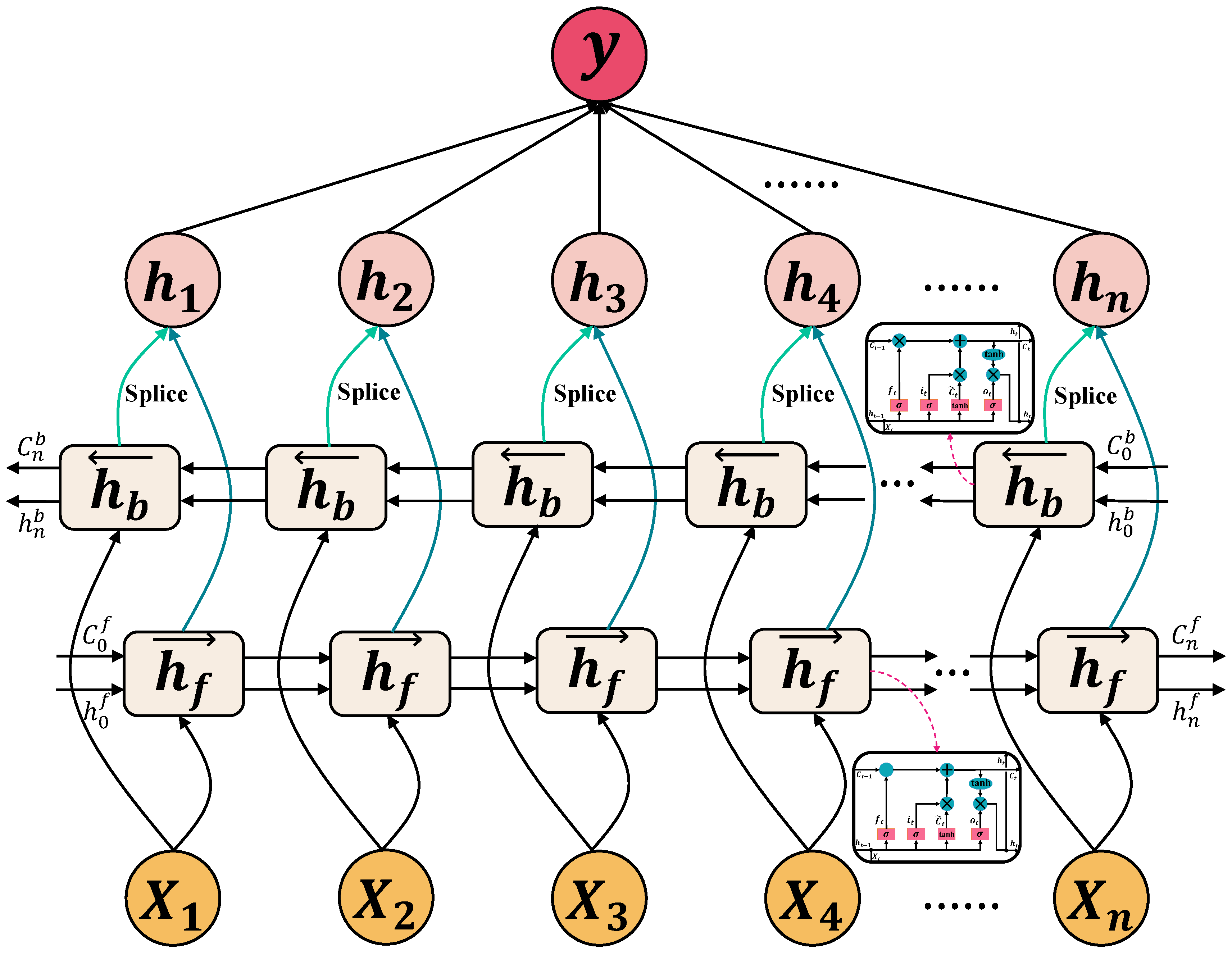
The structure of BiLSTM contains two LSTM layers, one to process the previous information and the other to process the future information [51], as shown in Figure 2. In addition, the direct sequence and the inverse sequence are concatenated with a single BiLSTM layer [52], as shown in Equations (9)–(11). BiLSTM can better capture the underlying contextual information after traversing the input data twice. In certain applications, BiLSTM can achieve great advantages, such as natural language processing and text analysis, where the translation of statements and the prediction of the next word in the input statement need to incorporate the information of the preceding and following contexts, as well as the time series of petroleum production.

$${\overrightarrow{h}}_t=LSTM(x_t,{\overrightarrow{h}}_{t-1})$$

(9)

$${{\displaystyle \overleftarrow{h}}}_t=LSTM(x_t,{\overleftarrow{h}}_{t+1})$$

(10)

$$y_t=g(W_{\overrightarrow{h}y},{\overleftarrow{h}}_t+W_{\overleftarrow{h}y},{\overleftarrow{h}}_t+b_y)$$

(11)

where $h_t$ denotes the output of the forward LSTM and the backward LSTM, $LSTM(\cdot )$ denotes functions of a standard LSTM, $W$ denotes the weights, $b$ denotes the bias, $g(\cdot )$ denotes the activation function, and $y_t$ denotes the final output of the hidden layer.

2.3. Proposed Model

Let $D={\left\{T_N\right\}}_{N=1}^{89}$ be the dataset in the training task, the dataset size of $D$ is 89, $T_N=\{x_1,x_2,x_3,\dots ,x_n\}$ is the nth task in the dataset $D$, $x_n=\{x_{n1},x_{n2},x_{n3},\dots ,x_{nt},\dots ,x_{n{l}_N}\}$ is the nth sequence within the current task, $x_{nt}$ is the sequence value at time step $t$, and $l_N$ is the length of the sequence in the current task. The proposed model uses $\{x_{n1},x_{n2},x_{n3},\dots ,x_{nt}\}$ to forecast the value $x_{n,t+1}$ for the next time step. The training and testing tasks in the method are different.

2.3.1. Framework Overview

In this paper, we use a training task and a test task to differentiate the datasets, where the training task contains 89 time series datasets, and the test task contains actual data from oil fields. The model is trained across the support set of the training task, the query set of the training task, and the support set of the test task. Figure 3 illustrates the problem formulation. $W=\{w_1,w_2,\dots ,w_m\}$, and the data of $m$ wells are used as the support set for the model in the testing task, which is used to adapt the model quickly. $Y=\{y_1,y_2,\dots ,y_n\}$ is the query set that is used to test the performance of the final model. In the training task, which is divided into support sets and query sets, $T_N$ are all different fields from each other. However, the time series in the tasks may be similar in dynamics to the time series in the target task. As an example, many time series contain trends, showing long-term trends of increasing or decreasing time series. In addition, time series related to human activities, e.g., strawberry production and electricity consumption, show trends in production and cyclical dynamics. The prediction performance of the target task can be improved by using the knowledge learned from various time series data.

2.3.2. Support Set and Query Set

In this research, the first n−1 time series of each task is used as the support set of $T_N$ ($T_N.Support$), which is used to learn the initialization parameters. The time series $\{x_{n-\mathrm{1,1}},x_{n-\mathrm{1,2}}\dots ,x_{n-1,t}\}$ within the support set of the training task $T_N$ is used as input. The base-learner forecasts the value $x_{n-1,t+1}$ of the next time step through the output of the feed-forward neural network and continuously adjusts the base-learner by passing and calculating the parameters. The nth time series is used as the query set of $T_N$ ($T_N.Query$), which is used to update the parameters of the meta-learner, to increase the generalization of the initialization parameters. When the model has finished training on $T_N.Support$, given the time series $\{x_{n1},x_{n2}\dots ,x_{nt}\}$ in $T_N.Query$, the prediction $x_{n,t+1}$ for the next time step is queried, and the error is calculated and recorded. In the training task, the length of time series in each task is equal, but the length of time series in different tasks is not equal. It is worth noting that the support set of the training task is used to allow the base-learner to learn the initialization parameters, the query set of the training task is designed to update the parameters of the meta-learner, the support set of test tasks is used to fine-tune the parameters of the meta-model, and the query set of the test task is designed to test the performance of the final model.

Figure 4 shows the mathematical descriptions of task $T_N$ and the test task. $x_n=\{x_{n1},x_{n2},\dots ,x_{nt},\dots ,x_{n{l}_N}\}$ is the nth time series in the training task $T_N$, $x_{nt}$ is the continuous value of the time scalar at time step $t$, and $l_N$ is the length of the sequence. $w_m=\{w_{m1},w_{m2},\dots ,w_{mt},\dots ,w_{m,l_{w_m}}\}\in W$ is the time series of the support set in the test task, and $l_{w_m}$ is the length of the time series of the well $w_m$. $y_n=\{y_{n1},y_{n2},\dots ,y_{nh},\dots ,y_{n,h+p}\}\in Y$ is the time series of the petroleum production in the query set Y. $\{y_{n1},y_{n2},\dots ,y_{nh}\}$ is used as an input to the sequence in the test to query for the prediction values $\{y_{n,h+1},\dots ,y_{n,h+p}\}$.

2.3.3. Base-Learner, Meta-Learner, and Training of Learners

The proposed model contains a base-learner (parameter of the network is $\theta$) and a meta-learner (parameter of the network is $\varphi$). The structure of meta-learner and base-learner is shown in Figure 5. We iteratively feed the base-learner with $\{x_{n1},x_{n2},\dots ,x_{nt}\}$ in $T_N.Support$ and then output, compute errors and gradients. The base-learner obtains the update parameter $\widehat{\theta }$ through iterative learning. Equation (12) illustrates the calculation of the error.

$$loss\left(\widehat{y},y\right)=\frac{1}{n}\sum {{(\widehat{y}}_i-y_i)}^2$$

(12)

where ${\widehat{y}}_i$ denotes the value forecasted by the neural network, and $y_i$ denotes the observed value.

The optimizer used is Adam [53], which optimizes base-learner as follows:

$$g_t={\nabla }_{\theta }·f\left({\theta }_t\right)$$

(13)

$$m_t={\beta }_1·m_{t-1}+\left(1-{\beta }_1\right)·g_t$$

(14)

$$V_t={\beta }_2·V_{t-1}+\left(1-{\beta }_2\right)·g_t^2$$

(15)

$${\widehat{m}}_t=\frac{m_t}{1-{\beta }_1^t}$$

(16)

$${\widehat{V}}_t=\frac{V_t}{1-{\beta }_2^t}$$

(17)

$${\theta }_{t+1}={\theta }_t-\frac{\alpha }{\sqrt{{\widehat{V}}_t}+\epsilon }·{\widehat{m}}_t$$

(18)

where $g_t$ denotes the gradient at time step $t$, $\theta$ is the weight parameter in the network, $f\left(\theta \right)$ is the stochastic objective function, ${\beta }_1$ and ${\beta }_2$ are the exponential decay rates of the first-order and second-order moments, respectively, $m_t$ and $v_t$ are the first-order method of moments and the second-order method of moments estimation of the gradient (which controls the direction of model updates and the learning rate), ${\widehat{m}}_t$ and ${\widehat{V}}_t$ are the updating corrections of $m_t$ and $V_t$, $\alpha$ is the learning rate, and $\epsilon$ is a constant.

Based on the updated base-learner, $T_N.Query$ is used to compute the error $l\left(\widehat{\theta }\right)$ and combine the errors on $T_N.Query$ to obtain $L\left(\varphi \right)$ as follows:

$$I=l_N-t$$

(19)

$$L\left(\varphi \right)={\sum }_{i=1}^I{l}^i\left(\widehat{\theta }\right)$$

(20)

where $I$ denotes the number of errors on $T_N.Query$, $t$ is the time step, $l_N$ is the length of the time series in $T_N.Query$, $L\left(\varphi \right)$ is the combination of errors on $T_N.Query$, and $l^n\left(\widehat{\theta }\right)$ is the error computed at each step on $T_N.Query$.

The gradient $G$ of $L\left(\varphi \right)$ over $\varphi$ is computed by Equation (21). The initialization parameter $\varphi$ is updated based on $L\left(\varphi \right)$ and $G$. Equation (22) illustrates the formula for updating $\varphi$. Notably, this gradient update is the second type of gradient update in the whole task, distinguishing it from the first update for the base-learner. Classical model-pretraining minimizes the loss of the current model and focuses on the performance in the present. However, the meta-learning strategy minimizes the loss of the subtasks after calculating the second time error, thus using the second type of gradient update of the meta-network. During the training of the subtask, the subtask changes from state zero to state one. Meta-learning expects the subtask to have a pretty small loss at state one, making TsrML more focused on the future potential of the parameters, which distinguishes it from model-pretraining. Figure 6 illustrates the meta-training logic of the training task.

$$G=\frac{\partial L\left(\varphi \right)}{\partial \varphi }$$

(21)

$$\varphi =\varphi -{\alpha }_{meta}·G$$

(22)

where $G$ denotes the gradient of $L\left(\varphi \right)$ over $\varphi$, $\varphi$ is the network parameter of the meta-learner, and ${\alpha }_{meta}$ is the learning rate of the meta-learner.

In the first stage of training, in order to avoid falling into the same training pattern as model-pretraining, the parameters of the meta-learner are assigned to a specific training task, updating the base-learner in it. Subsequently, computing the gradient and thus updating the meta-learner makes the meta-model focus more on the potential of the parameters rather than the performance of the task at hand. In the second stage, eight actual petroleum production sequences are fed into the meta-model for re-training, and the meta-model is adapted to the time series of the oil field with a small number of training sessions. As can be seen in Algorithm A1, for the meta-model to converge rapidly and efficiently, the gradient descent algorithm and the learning rate in updating the meta-learner parameters are different in the first and second stages (see Appendix A).

2.3.4. Test

The model proposed in this paper contains three phases of testing. The first phase of testing is the prediction made by the base-learner on the query set $T_N.Query$ in the training task, where the base-learner and meta-learner are not updated. Given the query time series $\{x_{n1},x_{n2},\dots ,x_{nt}\}\in x_n$ to forecast the predicted value $x_{n,t+1}$ at the next time step, calculate the error between the predicted value and the actual value after each step of prediction is completed, and $l_N-t$ error values can be obtained at the end of this time series. This stage aims to obtain the errors and combine them to update the meta-learner.

The point in time for the second phase of testing is after all the training tasks have been completed but have yet to be adapted to the target field when the model still needs to be fully mature. This phase aims to test the effectiveness of the current model on the UCR test set.

The third stage of the test is the prediction of petroleum production, given the query time series $y_n=\{y_{n1},y_{n2},\dots ,y_{nh}\}\in Y$ to forecast the future time series values $\{y_{n,h+1},y_{n,h+2},\dots ,y_{n,h+p}\}$. The purpose of this phase is to test the performance of the final model. In this paper, the third stage of testing considers several cases, which we illustrate in detail through the results in Section 4.1.

2.4. Reference Models

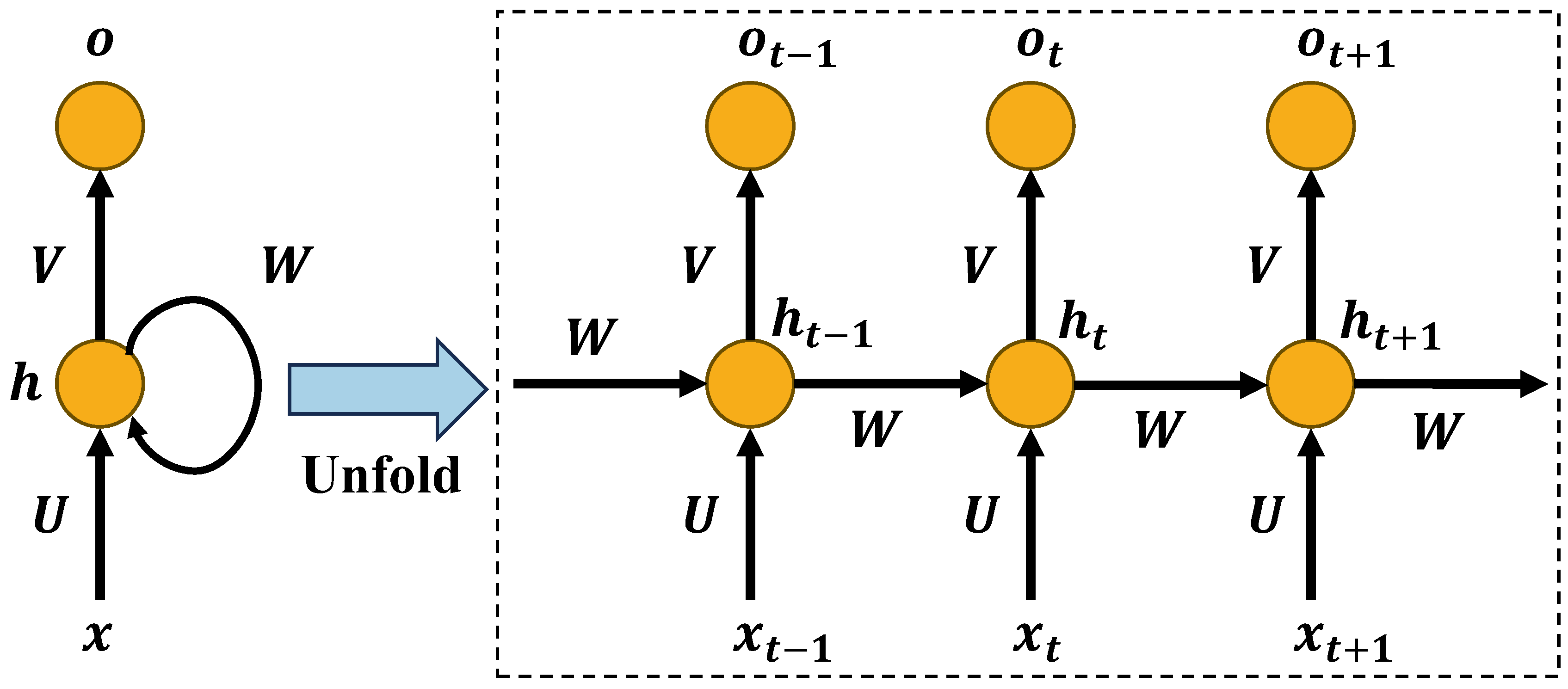
Three deep learning models are used as reference models: recurrent neural networks (RNN), LSTM, and BiLSTM. The architecture of RNN is shown in Figure 7, which is simpler than LSTM. For example, as shown in Equation (23), the current $h_t$ is related to the current input $x_t$ and the last hidden state $h_{t-1}$. The current output extracts the temporal features from $h_t$ using the linear transformation in Equation (24) [54]. However, the disadvantage of RNN is that it is not suitable for long sequence prediction without the complex gate functions that LSTM possesses.

$$h_t=tanh({Ux}_t+{Vh}_{t-1}+b_h)$$

(23)

$$o_t=W{h}_t+b_o$$

(24)

where $U$, $V$, and $W$ are the shared weights, and $b_h$ and $b_o$ are the shared deviations.

The hyperparameters for the reference models are presented in

Table 1. Hyperparameters in the reference models.

Model	Optimizer	Time Step	No. of Layers	Learning Rate	Hidden Size
RNN	Adam	12	3	10−3	32
LSTM	Adam	12	3	10−3	32
BiLSTM	Adam	12	1	10−3	$K_{\overrightarrow{h}}=K_{\overleftarrow{h}}=32$

. In addition, each reference model contains a dropout layer. The dropout rate is 0.1. To minimize statistical discrepancies, the test samples used in the reference models are identical to the ones used in TsrML.

3. Data Preprocessing

3.1. Data

For scientifically studying the performance of the proposed model, this paper uses the time series dataset from the UCR Time Series Classification Archive [55] in the training task. This dataset has already been divided into training and test sets, and there is no need to separate the range of the training and test sets separately. The datasets containing null values, time series lengths of less than 100, and time series numbers of less than 40 are omitted. Then, 89 time series datasets are obtained. The time series in the test task are taken from the actual petroleum production in Chinese oil fields, and the petroleum production is the monthly production, where the null values are replaced using the mean value of the corresponding well production. In the support set $W$ of the test task, the production data of an oil field ($W\in O_1$) in China are included. The query set $Y$ contains partial well data of two oil fields ($Y\in (O_1\cup O_2)$), and each of the wells contains few samples. The well data used were all taken from the period 2000 through 2022, with well data for the test sample beginning as early as 2017. We use the last 12 months of petroleum production as unknown data to be used as a test of the performance of the model. The features of the data in $O_2$ are invisible to the proposed model and are used to test the predictions of the model in other oil fields to examine whether the model satisfies the generalization requirements.

Table 2. The statistical information of the UCR dataset.

Dataset	Maximum No. of Rows	Minimum No. of Rows	Maximum No. of Columns	Minimum No. of Columns	No. of Series
Train	3636	16	2709	128	33,531
Test	3840	20	2709	128	90,431

and

Table 3. The statistical information of well production data.

Oil Field	Well	Count	Mean (m3/Month)	Max (m3/Month)	Min (m3/Month)	Standard Derivation
$O_1$	$w_1$	268	1258.8	7770.9	21.2	1434.7
	$w_2$	257	1081.5	7025.4	146.8	1086.0
	$w_3$	224	378.1	1325.7	76.3	198.7
	$w_4$	250	369.9	2905.6	18.3	248.5
	$w_5$	125	237.2	1703.2	8.0	257.7
	$w_6$	198	624.9	2647.5	8.1	391.6
	$w_7$	203	327.9	982.2	10.2	165.3
	$w_8$	139	720.4	2987.7	83.8	607.5
	$y_1$	72	1482.3	6024.5	191.9	1496.7
	$y_2$	54	1094.7	4437.0	251.8	909.8
	$y_3$	30	329.4	625.4	35.4	158.3
$O_2$	$y_4$	61	176.5	926.8	86.9	126.7
	$y_5$	54	471.9	2327.8	149.9	468.4
	$y_6$	39	776.5	1597.3	301.0	330.6

show detailed descriptions of the UCR dataset and information on oil wells.

In this paper, we investigate the relationship between the actual values of the petroleum time series and the actual values of the previous time step using the autocorrelation function (ACF) and the partial autocorrelation function (PACF). Figure 8 shows the ACF and PACF for the six series in the query set of the test task. The ACF plots show that the autocorrelation of the six series is insignificant, with the highest correlation being lag 1, which is not correlated from a lag average of 2.5 onwards. It is easy to notice from the PACF plots that in $y_1$–$y_5$ the first and second lags are significant (PACF for the first lag in $y_6$ is significant), and the rest of the lags are not significant. Two lagged values show a negative correlation in $y_2$ and $y_6$, respectively. Before the model started the training and testing tasks, all data were normalized, and the normalized data were compressed to a range between 0 and 1:

$$X^{\prime }=\frac{X-X_{min}}{X_{max}-X_{min}}$$

(25)

3.2. Experimental Setting

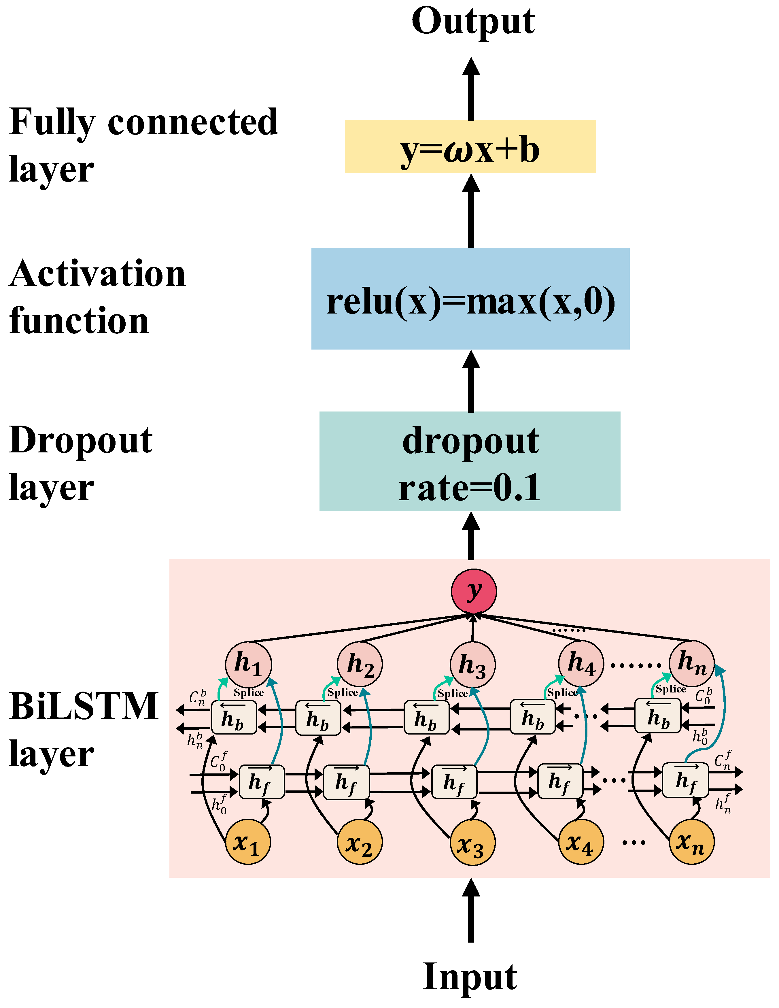
In this paper, the input time series is encoded using BiLSTM. Meta-learner and base-learner have the same network structure where the number of hidden units $K_{\overrightarrow{h}}=K_{\overleftarrow{h}}=32$, and the dropout rate in the neural network is 0.1. The activation function uses the Rectified Linear Unit (Relu):

$$Relu\left(x\right)=max(x,0)$$

(26)

The linear [56] is used to map the fully connected layer to the output, and the optimizer of the base-learner is Adam. The learning rate ${\alpha }_{meta}^1$ of meta-learner is ${10}^{-2}$, ${\alpha }_{meta}^2$ is ${10}^{-3}$. All models in this paper were architected using Pytorch in Python. All models were run on a computer with Intel Core i5-12400F CPU, RAM of 16 GB, and GPU of NVIDIA 3060.

3.3. Evaluation Indicators

In this paper, mean absolute error (MAE), mean square error (MSE), root mean square error (RMSE), and mean absolute percentage error (MAPE) are used in combination and are used to evaluate the performance of the model scientifically. The evaluation metrics are formulated as follows:

$$\mathrm{M}\mathrm{A}\mathrm{E}\left(X,h\right)=\frac{1}{m}{\sum }_{i=1}^m|h\left(x_i\right)-y_i|$$

(27)

$$\mathrm{M}\mathrm{S}\mathrm{E}\left(X,h\right)=\frac{1}{m}\sum _{i=1}^m{\left(h\left(x_i\right)-y_i\right)}^2$$

(28)

$$\mathrm{R}\mathrm{M}\mathrm{S}\mathrm{E}\left(X,h\right)=\sqrt{\frac{1}{m}\sum _{i=1}^m{\left(h\left(x_i\right)-y_i\right)}^2}$$

(29)

$$\mathrm{M}\mathrm{A}\mathrm{P}\mathrm{E}\left(X,h\right)=\frac{1}{m}{\sum }_{i=1}^m\left[\frac{|h\left(x_i\right)-y_i|}{y_i}\right]\times 100\mathrm{\%}$$

(30)

where $y_i$ denotes the actual value, $h\left(x_i\right)$ is the predicted, and $m$ is the number of sequence values.

4. Results and Discussion

Table 4. RMSE of the meta-model at the end of the training task on the test set of 89 time series datasets. The last row shows the average root mean square error for all UCR test tasks.

Dataset	Error	Dataset	Error
ACSF1	0.409	Lightning2	0.024
Adiac	0.005	Lightning7	0.041
ArrowHead	0.008	Mallat	0.005
Beef	0.006	Meat	0.003
BirdChicken	0.005	MixedShapesRegularTrain	0.003
BME	0.024	MixedShapesSmallTrain	0.003
Car	0.003	NonInvasiveFetalECGThorax1	0.002
CBF	0.135	NonInvasiveFetalECGThorax2	0.001
ChlorineConcentration	0.091	OliveOil	0.007
CinCECGTorso	0.004	OSULeaf	0.007
Coffee	0.011	Phoneme	0.040
Computers	0.060	PigAirwayPressure	0.013
CricketX	0.031	PigArtPressure	0.006
CricketY	0.031	PigCVP	0.018
CricketZ	0.032	Plane	0.019
DiatomSizeReduction	0.003	PowerCons	0.052
Earthquakes	0.197	RefrigerationDevices	0.108
ECG5000	0.021	ScreenType	0.044
ECGFiveDays	0.009	SemgHandGenderCh2	0.090
EOGHorizontalSignal	0.005	SemgHandMovementCh2	0.089
EOGVerticalSignal	0.005	SemgHandSubjectCh2	0.087
EthanolLevel	0.006	ShapeletSim	0.329
FaceAll	0.050	ShapesAll	0.005
FaceFour	0.042	SmallKitchenAppliances	0.023
FacesUCR	0.075	StarLightCurves	0.004
FiftyWords	0.007	Strawberry	0.005
Fish	0.002	SwedishLeaf	0.023
FordA	0.027	Symbols	0.003
FordB	0.025	ToeSegmentation1	0.025
FreezerRegularTrain	0.012	ToeSegmentation2	0.014
FreezerSmallTrain	0.012	Trace	0.018
Fungi	0.013	TwoPatterns	0.118
GunPointAgeSpan	0.006	UMD	0.021
GunPointMaleVersusFemale	0.006	UWaveGestureLibraryAll	0.008
GunPointOldVersusYoung	0.007	UWaveGestureLibraryX	0.005
GunPoint	0.006	UWaveGestureLibraryY	0.005
Ham	0.016	UWaveGestureLibraryZ	0.005
HandOutlines	0.002	Wafer	0.015
Haptics	0.005	Wine	0.003
Herring	0.003	WordSynonyms	0.007
HouseTwenty	0.027	WormsTwoClass	0.011
InlineSkate	0.004	Worms	0.011
InsectEPGRegularTrain	0.026	Yoga	0.003
InsectEPGSmallTrain	0.026	Average	0.031

shows the root mean square error obtained by testing the model obtained after the completion of the training task on the UCR test set, and this result shows that the proposed meta-model for time series forecasting can obtain low errors on 89 time series datasets. Moreover, 12 examples are shown in Figure 9, which show the predicted and actual value curves of the model on the UCR test set. Notably, the model can obtain positive results on 89 time series datasets where features have been seen.

4.1. Results of Comparison

In this section, the results are divided into three case studies for discussion, and the results of each case study are presented. Notably, the results presented in each case study are the results and performance of the corresponding model on the query set in the test task rather than the training task. It has been widely proven that only the results based on unknown data have real evaluative value, not the data the model already learned during training [57].

4.1.1. Case Study 1: Using Different Basic Models in the Proposed Methodology

Using different basic models may cause differences in the effectiveness of the proposed meta-learning approach, so RNN and LSTM are used as the basic models for reference. Therefore, the performance of TsrML using different basic models is investigated. The training methods used in this case study and all datasets (including training and test tasks) are identical. The relationship between the prediction results of the meta-models trained using different basic models and the original production data is shown in Figure 10, and the test errors are listed in

Table 5. Test errors of TsrML trained using different basic models.

Well	Basic Model	MAE	MSE	RMSE	MAPE(%)
$y_1$	RNN	0.0669	0.0069	0.0829	3.5790
	LSTM	0.0702	0.0070	0.0833	3.1484
	BiLSTM	0.0658	0.0068	0.0828	2.4408
$y_2$	RNN	0.0772	0.0081	0.0901	3.4786
	LSTM	0.0669	0.0075	0.0864	2.3589
	BiLSTM	0.0438	0.0044	0.0667	2.1262
$y_3$	RNN	0.3417	0.1479	0.3845	1.2008
	LSTM	0.2862	0.1673	0.4090	0.9930
	BiLSTM	0.1473	0.0508	0.2254	0.3203

. In addition, the time spent on training using different basic models is presented in

Table 6. Time spent on training using different basic models.

Basic Model	Training Time
RNN	4 h’19 min
LSTM	4 h’21 min
BiLSTM	4 h’38 min

.

Figure 10 and Table 5 show that the basic model of TsrML using BiLSTM performs better than RNN or LSTM. The performance of its evaluation metrics is not only better than that of RNN and LSTM, but the TsrML model trained using BiLSTM is also better able to describe the time series curve of petroleum production.

4.1.2. Case Study 2: Comparison of Our Model with Traditional Deep Learning Methods

This case study aims to compare the meta-learning method with the traditional machine learning methods. Notably, the training set of the traditional method is just a small amount of data that $y_n$ has. The traditional methods are trained based on the historical data of $y_n$ and predict the future production data, meaning that the model is trained on the dataset with few samples.

The traditional deep learning methods contain three models: RNN, LSTM, and BiLSTM. The relationships between the predicted production of the three models on the three wells, the results predicted by TsrML, and the original production data are shown in Figure 11. It is worth noting that the production predicted by TsrML is closer to the actual production than predicted by the traditional methods.

In addition, we go through continuous parameter tuning to find the optimal parameters of the three models in the traditional method and determine the corresponding hyperparameters.

Table 7. Best results of traditional methods under different epochs. The metrics in the table are root mean squared errors.

Model	Well	No. of Epochs	Train	Test
RNN	$y_1$	100	0.1370	0.3067
		150	0.1218	0.2163
		200	0.1140	0.2452
	$y_2$	100	0.1932	0.3423
		150	0.1281	0.2281
		200	0.1278	0.2610
	$y_3$	50	0.0771	0.3646
		200	0.0225	0.3418
		300	0.0149	0.3417
LSTM	$y_1$	50	0.0642	0.0544
		200	0.0330	0.0180
		300	0.0411	0.0430
	$y_2$	50	0.0815	0.0581
		200	0.0621	0.0578
		300	0.0603	0.0554
	$y_3$	50	0.2012	0.5859
		100	0.1435	0.5049
		150	0.1211	0.6078
BiLSTM	$y_1$	50	0.0720	0.2176
		150	0.0321	0.0956
		250	0.0295	0.0992
	$y_2$	50	0.0830	0.2341
		150	0.0489	0.0564
		250	0.0295	0.0570
	$y_3$	50	0.0034	0.3544
		100	0.0011	0.3852
		150	0.0004	0.4042

shows the performance metrics of the three models under different epochs.

Table 8. The errors of three well production data in $O_1$ using traditional deep learning methods and the proposed method.

Well	Model	MAE	MSE	RMSE	MAPE(%)
$y_1$	RNN	0.1109	0.0124	0.1115	5.0571
	LSTM	0.0813	0.0068	0.0822	3.8725
	BiLSTM	0.1345	0.0234	0.1531	5.6475
	TsrML	0.0711	0.0061	0.0785	3.3812
$y_2$	RNN	0.2216	0.0520	0.2281	8.7203
	LSTM	0.0687	0.0058	0.0763	3.2038
	BiLSTM	0.0595	0.0044	0.0667	2.7080
	TsrML	0.0438	0.0044	0.0667	2.1262
$y_3$	RNN	0.2938	0.1168	0.3418	1.0229
	LSTM	0.4468	0.2550	0.5050	1.6173
	BiLSTM	0.3333	0.1484	0.3852	1.1219
	TsrML	0.1473	0.0508	0.2254	0.3203

lists the test errors of the traditional deep learning methods and the TsrML method on the time series of the three wells. The RMSE and MAPE of the TsrML are as low as 0.0667 and 0.3203, as high as 0.2254 and 3.3812. Considering the four metrics together with the prediction curves in Figure 11, the results show that the TsrML outperforms the traditional training methods in few-shot prediction. Notably, the numbers of epochs for the traditional methods in Figure 11 and Table 8 are taken from the best results in Table 7.

4.1.3. Case Study 3: Testing the Generalization of the Proposed Meta-Method

After training on the support set $W$ of the test task, the model went through the final parameter fine-tuning, and with that, the final model was obtained. Subsequently, samples from the oil field $O_1$ are used for testing and comparing the effects in case study 1 and case study 2, where $W\in O_1$ and $\{y_1,y_2,y_3\}\in O_1$. However, the ultimate goal is to train a petroleum time series forecasting model that is not limited to a single well, which cannot be illustrated by merely testing on data from different wells within the same field.

Therefore, in order to evaluate the model fairly, we experiment with data from another oil field $O_2$, where $O_1$ and $O_2$ are oil fields in two different places in China ($O_1\ne O_2$). The relationship between the actual production data and the predictions of the TsrML model is shown in Figure 12.

Table 9. The errors of three well production data in $O_2$ using TsrML.

Well	Model	MAE	MSE	RMSE	MAPE(%)
$y_4$	RNN	0.3670	0.2123	0.4608	12.6789
	LSTM	0.3548	0.1356	0.3683	12.2480
	BiLSTM	0.3417	0.1459	0.3820	9.7759
	TsrML	0.1370	0.0370	0.1924	3.5760
$y_5$	RNN	0.3966	0.1607	0.4009	12.5077
	LSTM	0.2485	0.1207	0.3475	9.9458
	BiLSTM	0.1790	0.0342	0.1849	6.8870
	TsrML	0.0953	0.0131	0.1142	3.9250
$y_6$	RNN	0.3657	0.1413	0.3758	2.6400
	LSTM	0.3448	0.1879	0.4334	2.6907
	BiLSTM	0.3748	0.1484	0.3852	2.6821
	TsrML	0.2702	0.1074	0.3277	1.1352

shows the evaluation metrics of the TsrML model on the three wells within the $O_2$ field. The lowest RMSE of the TsrML on the three wells in $O_2$ is 0.1142, the lowest MAPE is 1.1352, and the lowest MAE is 0.0953.

In addition, Figure 13 shows the regression performance of various models. The figure includes the actual and predicted values for the six wells, and the predicted values contain historical fitting values of different models and the predicted values for the next 12 months. Among them, the historical fitting values of RNN, LSTM, and BiLSTM are optimal results obtained after multiple training sessions on each sequence. However, no training was performed by TsrML on these time series ($y_1$–$y_6$). Including Figure 13, all test results for TsrML are the results of testing the model obtained after fast adaptation on $W$ without training on the query set in the test task. Both RNN and LSTM have the lowest prediction accuracy, with most of the data having an absolute error of more than 300 m³ and the largest absolute errors reaching 1944 m³ and 1623 m³. Only a few absolute errors of BiLSTM exceed 300 m³, with the largest absolute error reaching 752 m³. However, the network structure of BiLSTM is very suitable for predicting time series, which helps its predictions look good in the scatterplot, and the data close to the 45° reference line within the error interval of $\pm$300 m³ are already-known data that BiLSTM was trained on several times. Most of the unknown future data exceeded the error interval. Only one data point in TsrML has an absolute error of 654 m³ over 300 m³ scattered below the 45° straight line, and the rest of the data are within the $\pm$300 m³ error interval, indicating the highest prediction accuracy. The data point of well $y_5$ in the 25th month is 2327.8 m³ with an absolute error of 654 m³, while the actual data before and after the 25th month are below 2000 m³. Due to the insufficient self-injection capacity, this well was intermittently opened in the early period of production, but the result was poor. After that, the pump was changed, and production was intermittent with insufficient fluid supply. At the end of the 23rd month, water injection started to produce oil, and oil production reached its maximum in the 25th month, after which water injection became less effective. Since the change in production measures resulted in a significant increase in the value in the 25th month in well $y_5$, it did not affect the performance of TsrML.

Overall, according to the data from the six wells, the accuracy of the TsrML model is significantly better than that of the three traditional deep learning models, further demonstrating the effectiveness of the meta-method.

4.2. Results Analysis and Discussion

In the work of this paper, we aim to combine the method of meta-learning with petroleum production prediction so as to forecast the time series of crude petroleum production effectively. By utilizing the property that BiLSTM is more suitable for the analysis of time series than LSTM or RNN, the time series of monthly petroleum production are effectively studied, which provides guidance for the production in the oil field site. Three case studies were summarized to illustrate the performance of the proposed model, which compared the production prediction results of TsrML models trained using different basic models and also evaluated the prediction results of traditional deep learning methods and TsrML. To test the generalization ability of TsrML, the time series from different oil fields are used to evaluate the effectiveness of TsrML.

In case study 1, from the prediction curves of the three wells in Figure 9 for the next 12 months, the meta-model trained using BiLSTM as the basic model fits the actual production curves better than the meta-model trained using RNN and LSTM. As known, the lower the values of the evaluation metrics (MAE, MSE, RMSE, MAPE), the better the performance. The different evaluation metrics of the TsrML model trained using three different basic models for the three wells in $O_1$ are shown in Table 5 and Figure 14. The MAE, RMSE, and MAPE of the TsrML model trained using BiLSTM are 0.0658, 0.0828, and 2.4408 for $y_1$, its MAE, RMSE, and MAPE are 0.0438, 0.0667, and 2.1262 for $y_2$, its MAE, RMSE, and MAPE are 0.1473, 0.2254, and 0.3203 for $y_3$. The TsrML model obtained by meta-training using BiLSTM as the basic model has the lowest MAE, MSE, RMSE, and MAPE compared to the TsrML model trained using RNN and LSTM. The possibility exists that information at a given moment in a petroleum time series is related to historical and future information, and bidirectional inputs can provide neural networks with additional hidden information about the preceding and following contexts. Therefore, compared to unidirectional networks, bidirectional networks can learn more adequately and represent the complex features of time series more efficiently, especially for data with significant nonlinear characteristics, such as production data. In this case, the results show that BiLSTM matches the proposed method better than RNN and LSTM. Moreover, it can be verified that bidirectional LSTM is more applicable to time series problems than unidirectional LSTM [58].

In case study 2, the traditional deep learning methods were compared with the TsrML method. Figure 11 shows that the prediction performance of TsrML is superior to that of the traditional methods both for known historical data and unknown data. It is worth noting that due to the few samples available for training of the traditional methods, it can be seen from Figure 11 that its future prediction curves on both $y_1$ and $y_2$ are horizontal, which cannot effectively illustrate the trend of the production sequence. For the few-shot data within the $O_1$ oil field, the performance of the proposed meta-learning method outperforms the traditional methods, both in terms of the fit of the sequence curves and the effective illustrative properties of the production trend. According to the evaluation metrics in Table 8 and Figure 15, it can be noticed that for $y_1$ and $y_2$, the evaluation metrics of TsrML are not always advantageously significant. For $y_1$, the value of MAE 0.0711 and the value of RMSE 0.0785 for the TsrML model are slightly lower than the optimal values of 0.0813 and 0.0822 for the LSTM model. For $y_2$, the value of MAE 0.0438 for TsrML is slightly lower than the optimal value of 0.0595 for the BiLSTM model. And the RMSE value of TsrML after retaining four decimals is the same as the RMSE of BiLSTM. However, it can be noticed from (a) and (b) of Figure 11 that the future sequence curves predicted by the traditional method are exactly around the actual curves and show a nearly horizontal trend. Although the performance of this prediction seems to be good in terms of error data, an effective guidance cannot be realized. The curve of TsrML is more indicative of fluctuations and trends than traditional methods. Therefore, the TsrML model can be well used for forecasting production under the problem of few-shot samples, which provides practical and reliable guidance for decision-making in petroleum production in a meaningful way.

The proposed TsrML aims to solve the problem of the size of petroleum time series samples not being enough to support the good prediction performance of traditional deep learning methods. Therefore, to evaluate the model more comprehensively, in case study 3, the data from the $O_2$ oil field were utilized to objectively evaluate the ability of the TsrML method to fit the history of different oil field data and to forecast the unknown sequences. According to Table 9 and Figure 16, it can be seen that TsrML has good prediction performance for data within the $O_2$ oil field. For $y_4$, the values of MAE, RMSE, and MAPE for TsrML are 0.137, 0.1924, and 3.576. For $y_5$, the values of MAE, RMSE, and MAPE for TsrML are 0.0953, 0.1142, and 3.925. Compared with the performance of the reference models on the two wells, the advantage of TsrML is significant. From (b) of Figure 12, it can be observed that the curve of RNN is overall lower than the actual curve, the curve of BiLSTM is higher than the actual overall, and the curve of LSTM moves away from the actual curve with the increasing number of months, and the prediction error in the latter part of the curve gradually increases. Although the RMSE value of 0.3277 for TsrML is not significantly lower than that of 0.3758 for RNN. However, it is obvious from (c) of Figure 12 that the prediction curves of the traditional methods are difficult to illustrate the production trend of $y_6$, in which the traditional deep learning models cannot learn efficiently enough due to the few samples available for training. The prediction curve of RNN tends to be horizontal, the prediction curve of LSTM presents a quadratic function, and the prediction curve of BiLSTM shows insignificant fluctuations; its curve does not fit the actual situation and cannot be realized for guidance.

In case studies 2 and 3, the superior performance of TsrML on error metrics is not always significant. This is normal since traditional methods are prone to overfitting in the few-shot problem, and as the difference between the first value predicted and the last value of the historical data is generally not large, the prediction curves are prone to be horizontal around the actual curve. In contrast, the sequence curves predicted by TsrML have fluctuations. In this paper, the percentage metric MAPE and relative error $E_R$ were used to assist in the evaluation. As known, the evaluation of deep learning models should not focus on a particular metric but on a combination of multiple metrics and the practicability of the forecasted curves to be evaluated objectively.

Notably, the total sequence lengths of wells $y_3$ and $y_6$ are 30 and 39, which are shorter than those of $y_1$, $y_2$, $y_4$, and $y_5$. The error metrics of TsrML for $y_3$ and $y_6$ are lower than those of the traditional methods, and the advantages are more significant. This means that the smaller the sample size, the more significant the performance advantage of TsrML compared to traditional training methods. In contrast, traditional methods are prone to overfitting, and the curves formed by their predicted sequence values hardly describe the trend of petroleum production. The results of these cases showed that TsrML is more effective than traditional methods in forecasting the future production of petroleum and describing the trend of the production time series when faced with the problem of few-shot.

5. Conclusions

In this paper, we proposed a time series forecasting approach based on meta-learning for petroleum production under few-shot samples, which used a bidirectional long short-term memory (BiLSTM) recurrent network as the basic model. In this paper, the method was divided into a training task and a test task, and each task contained its own support set and query set to perform a complete set of meta-training, which is denoted as TsrML. Notably, the training task contained 89 time series datasets. The test task included eight wells used to adapt to the petroleum time series quickly and six wells in two oil fields used to test the performance of the final model. The experience in this paper demonstrated that traditional deep learning training methods can hardly perform well in forecasting petroleum time series with few samples, and the results are prone to overfitting. However, the proposed meta-learning method can alleviate the limitations of traditional methods.

Notably, the proposed TsrML model outperformed the traditional approaches of RNN, LSTM, and BiLSTM in the two case studies described in this paper, where there was a significant difference in the effectiveness of the forecasted sequence curves. In addition, this paper conducted a case study of the proposed method using different basic models. The experience proved that the proposed method using BiLSTM as the basic model for training is superior to LSTM and RNN. In addition, the advantages of BiLSTM over LSTM in time series problems were also highlighted.

The superior performance and validity of the predictions showed that the proposed method can capture the nonlinear characteristics of the petroleum series and show the future trend of the petroleum production series. Therefore, TsrML is suitable for application to time series forecasting problems in oil fields and is a promising method. In the future work plan, we will investigate the application of TsrML to time series forecasting that includes multiple variables.

References

- Lu, H.; Huang, K.; Azimi, M.; Guo, L. Blockchain Technology in the Oil and Gas Industry: A Review of Applications, Opportunities, Challenges, and Risks. IEEE Access 2019, 7, 41426–41444. [Google Scholar] [CrossRef]
- Pan, S.; Yang, B.; Wang, S.; Guo, Z.; Wang, L.; Liu, J.; Wu, S. Oil well production prediction based on CNN-LSTM model with self-attention mechanism. Energy 2023, 284, 128701. [Google Scholar] [CrossRef]
- Karevan, Z.; Suykens, J.A. Transductive LSTM for time-series prediction: An application to weather forecasting. Neural Netw. 2020, 125, 1–9. [Google Scholar] [CrossRef]
- Livieris, I.E.; Pintelas, E.; Pintelas, P. A CNN–LSTM model for gold price time-series forecasting. Neural Comput. Appl. 2020, 32, 17351–17360. [Google Scholar] [CrossRef]
- Yang, H.; Huang, K.; King, I.; Lyu, M.R. Localized support vector regression for time series prediction. Neurocomputing 2009, 72, 2659–2669. [Google Scholar] [CrossRef]
- Chimmula, V.K.R.; Zhang, L. Time series forecasting of COVID-19 transmission in Canada using LSTM networks. Chaos Solitons Fractals 2020, 135, 109864. [Google Scholar] [CrossRef]
- McCoy, T.H.; Pellegrini, A.M.; Perlis, R.H. Assessment of Time-Series Machine Learning Methods for Forecasting Hospital Discharge Volume. JAMA Netw. Open 2018, 1, e184087. [Google Scholar] [CrossRef]
- Abbasimehr, H.; Shabani, M.; Yousefi, M. An optimized model using LSTM network for demand forecasting. Comput. Ind. Eng. 2020, 143, 106435. [Google Scholar] [CrossRef]
- Nguyen, H.; Tran, K.P.; Thomassey, S.; Hamad, M. Forecasting and Anomaly Detection approaches using LSTM and LSTM Autoencoder techniques with the applications in supply chain management. Int. J. Inf. Manag. 2021, 57, 102282. [Google Scholar] [CrossRef]
- Sun, J.; Di, L.P.; Sun, Z.H.; Shen, Y.L.; Lai, Z.L. County-Level Soybean Yield Prediction Using Deep CNN-LSTM Model. Sensors 2019, 19, 4363. [Google Scholar] [CrossRef]
- Gasparin, A.; Lukovic, S.; Alippi, C. Deep learning for time series forecasting: The electric load case. Caai Trans. Intell. Technol. 2022, 7, 1–25. [Google Scholar] [CrossRef]
- Chen, J.; Zeng, G.-Q.; Zhou, W.; Du, W.; Lu, K.-D. Wind speed forecasting using nonlinear-learning ensemble of deep learning time series prediction and extremal optimization. Energy Convers. Manag. 2018, 165, 681–695. [Google Scholar] [CrossRef]
- Lu, X.; Lin, P.; Cheng, S.; Lin, Y.; Chen, Z.; Wu, L.; Zheng, Q. Fault diagnosis for photovoltaic array based on convolutional neural network and electrical time series graph. Energy Convers. Manag. 2019, 196, 950–965. [Google Scholar] [CrossRef]
- Vida, G.; Shahab, M.D.; Mohammad, M. Smart Proxy Modeling of SACROC CO2-EOR. Fluids 2019, 4, 85. [Google Scholar] [CrossRef]
- Chen, G.; Tian, H.; Xiao, T.; Xu, T.; Lei, H. Time series forecasting of oil production in Enhanced Oil Recovery system based on a novel CNN-GRU neural network. Geoenergy Sci. Eng. 2024, 233, 212528. [Google Scholar] [CrossRef]
- Sagheer, A.; Kotb, M. Time series forecasting of petroleum production using deep LSTM recurrent networks. Neurocomputing 2019, 323, 203–213. [Google Scholar] [CrossRef]
- Bollapragada, R.; Mankude, A.; Udayabhanu, V. Forecasting the price of crude oil. Decision 2021, 48, 207–231. [Google Scholar] [CrossRef]
- Ma, X.; Liu, Z. Predicting the oil production using the novel multivariate nonlinear model based on Arps decline model and kernel method. Neural Comput. Appl. 2018, 29, 579–591. [Google Scholar] [CrossRef]
- Chithra Chakra, N.; Song, K.-Y.; Gupta, M.M.; Saraf, D.N. An innovative neural forecast of cumulative oil production from a petroleum reservoir employing higher-order neural networks (HONNs). J. Pet. Sci. Eng. 2013, 106, 18–33. [Google Scholar] [CrossRef]
- Fan, D.Y.; Sun, H.; Yao, J.; Zhang, K.; Yan, X.; Sun, Z.X. Well production forecasting based on ARIMA-LSTM model considering manual operations. Energy 2021, 220, 119708. [Google Scholar] [CrossRef]
- Abdullayeva, F.; Imamverdiyev, Y. Development of oil production forecasting method based on deep learning. Stat. Optim. Inf. Comput. 2019, 7, 826–839. [Google Scholar] [CrossRef]
- Aizenberg, I.; Sheremetov, L.; Villa-Vargas, L.; Martinez-Muñoz, J. Multilayer neural network with multi-valued neurons in time series forecasting of oil production. Neurocomputing 2016, 175, 980–989. [Google Scholar] [CrossRef]
- Shin, H.; Hou, T.; Park, K.; Park, C.-K.; Choi, S. Prediction of movement direction in crude oil prices based on semi-supervised learning. Decis. Support Syst. 2013, 55, 348–358. [Google Scholar] [CrossRef]
- Song, X.; Liu, Y.; Xue, L.; Wang, J.; Zhang, J.; Wang, J.; Jiang, L.; Cheng, Z. Time-series well performance prediction based on Long Short-Term Memory (LSTM) neural network model. J. Pet. Sci. Eng. 2020, 186, 106682. [Google Scholar] [CrossRef]
- Schmidhuber, J. A neural network that embeds its own meta-levels. In Proceedings of the IEEE International Conference on Neural Networks, San Francisco, CA, USA, 28 March–1 April 1993; pp. 407–412. [Google Scholar]
- Thrun, S. Lifelong Learning Algorithms. In Learning to Learn; Thrun, S., Pratt, L., Eds.; Springer: Boston, MA, USA, 1998; pp. 181–209. [Google Scholar] [CrossRef]
- Jamal, M.A.; Qi, G.-J. Task agnostic meta-learning for few-shot learning. In Proceedings of the 2019 IEEE/CVF Conference on Computer Vision and Pattern Recognition (CVPR), Long Beach, CA, USA, 15–20 June 2019; pp. 11719–11727. [Google Scholar]
- Prudêncio, R.B.; Ludermir, T.B. Meta-learning approaches to selecting time series models. Neurocomputing 2004, 61, 121–137. [Google Scholar] [CrossRef]
- Schweighofer, N.; Doya, K. Meta-learning in reinforcement learning. Neural Netw. 2003, 16, 5–9. [Google Scholar] [CrossRef] [PubMed]
- Widmer, G. Tracking context changes through meta-learning. Mach. Learn. 1997, 27, 259–286. [Google Scholar] [CrossRef]
- Hu, J.; Heng, J.; Tang, J.; Guo, M. Research and application of a hybrid model based on Meta learning strategy for wind power deterministic and probabilistic forecasting. Energy Convers. Manag. 2018, 173, 197–209. [Google Scholar] [CrossRef]
- Van Engelen, J.E.; Hoos, H.H. A survey on semi-supervised learning. Mach. Learn. 2020, 109, 373–440. [Google Scholar] [CrossRef]
- Gupta, G.; Yadav, K.; Paull, L. Look-ahead meta learning for continual learning. Adv. Neural Inf. Process. Syst. 2020, 33, 11588–11598. [Google Scholar]
- Hospedales, T.; Antoniou, A.; Micaelli, P.; Storkey, A. Meta-Learning in Neural Networks: A Survey. IEEE Trans. Pattern Anal. Mach. Intell. 2022, 44, 5149–5169. [Google Scholar] [CrossRef] [PubMed]
- Li, X.C.; Ma, X.F.; Xiao, F.C.; Xiao, C.; Wang, F.; Zhang, S.C. Small-Sample Production Prediction of Fractured Wells Using Multitask Learning. SPE J. 2022, 27, 1504–1519. [Google Scholar] [CrossRef]
- Wang, Y.; Yu, C.; Hou, J.; Chu, S.; Zhang, Y.; Zhu, Y. ARIMA model and few-shot learning for vehicle speed time series analysis and prediction. Comput. Intell. Neurosci. 2022, 2022, 252682. [Google Scholar] [CrossRef]
- Finn, C.; Abbeel, P.; Levine, S. Model-agnostic meta-learning for fast adaptation of deep networks. In Proceedings of the 34th International Conference on Machine Learning, Sydney, Australia, 6–11 August 2017; pp. 1126–1135. [Google Scholar]
- Xu, Z.; Chen, X.; Tang, W.; Lai, J.; Cao, L. Meta weight learning via model-agnostic meta-learning. Neurocomputing 2021, 432, 124–132. [Google Scholar] [CrossRef]
- Ravi, S.; Larochelle, H. Optimization as a model for few-shot learning. In Proceedings of the 2017 International Conference on Learning Representations, Toulon, France, 24–26 April 2017. [Google Scholar]
- Munkhdalai, T.; Yu, H. Meta networks. In Proceedings of the International Conference on Machine Learning, Sydney, Australia, 6–11 August 2017; pp. 2554–2563. [Google Scholar]
- Xu, H.; Wang, J.; Li, H.; Ouyang, D.; Shao, J. Unsupervised meta-learning for few-shot learning. Pattern Recognit. 2021, 116, 107951. [Google Scholar] [CrossRef]
- Li, X.; Sun, Z.; Xue, J.-H.; Ma, Z. A concise review of recent few-shot meta-learning methods. Neurocomputing 2021, 456, 463–468. [Google Scholar] [CrossRef]
- Qiu, X.; Sun, T.; Xu, Y.; Shao, Y.; Dai, N.; Huang, X. Pre-trained models for natural language processing: A survey. Sci. China Technol. Sci. 2020, 63, 1872–1897. [Google Scholar] [CrossRef]
- Wang, J.X. Meta-learning in natural and artificial intelligence. Curr. Opin. Behav. Sci. 2021, 38, 90–95. [Google Scholar] [CrossRef]
- Nichol, A.; Achiam, J.; Schulman, J. On First-Order Meta-Learning Algorithms. arXiv, 2018; arXiv:1803.02999. [Google Scholar] [CrossRef]
- Vinyals, O.; Blundell, C.; Lillicrap, T.; Wierstra, D. Matching networks for one shot learning. Adv. Neural Inf. Process. Syst. 2016, 29, 3637–3645. [Google Scholar]
- Antoniou, A.; Edwards, H.; Storkey, A. How to train your MAML. In Proceedings of the International Conference on Learning Representations, New Orleans, LA, USA, 6–9 May 2019. [Google Scholar]
- Sabzipour, B.; Arsenault, R.; Troin, M.; Martel, J.-L.; Brissette, F.; Brunet, F.; Mai, J. Comparing a long short-term memory (LSTM) neural network with a physically-based hydrological model for streamflow forecasting over a Canadian catchment. J. Hydrol. 2023, 627, 130380. [Google Scholar] [CrossRef]
- Song, B.; Liu, Y.; Fang, J.; Liu, W.; Zhong, M.; Liu, X. An optimized CNN-BiLSTM network for bearing fault diagnosis under multiple working conditions with limited training samples. Neurocomputing 2024, 574, 127284. [Google Scholar] [CrossRef]
- Graves, A.; Schmidhuber, J. Framewise phoneme classification with bidirectional LSTM and other neural network architectures. Neural Netw. 2005, 18, 602–610. [Google Scholar] [CrossRef] [PubMed]
- Sharfuddin, A.A.; Tihami, M.N.; Islam, M.S. A Deep Recurrent Neural Network with BiLSTM model for Sentiment Classification. In Proceedings of the 2018 International Conference on Bangla Speech and Language Processing (ICBSLP), Sylhet, Bangladesh, 21–22 September 2018; pp. 1–4. [Google Scholar]
- da Silva, D.G.; Meneses, A.A.d.M. Comparing Long Short-Term Memory (LSTM) and bidirectional LSTM deep neural networks for power consumption prediction. Energy Rep. 2023, 10, 3315–3334. [Google Scholar] [CrossRef]
- Kingma, D.P.; Ba, J. Adam: A method for stochastic optimization. arXiv, 2014; arXiv:1412.6980. [Google Scholar] [CrossRef]
- Shan, F.; He, X.; Armaghani, D.J.; Sheng, D. Effects of data smoothing and recurrent neural network (RNN) algorithms for real-time forecasting of tunnel boring machine (TBM) performance. J. Rock Mech. Geotech. Eng. 2023. [Google Scholar] [CrossRef]
- Dau, H.A.; Bagnall, A.; Kamgar, K.; Yeh, C.-C.M.; Zhu, Y.; Gharghabi, S.; Ratanamahatana, C.A.; Keogh, E. The UCR time series archive. IEEE/CAA J. Autom. Sin. 2019, 6, 1293–1305. [Google Scholar] [CrossRef]
- Linear. Available online: https://pytorch.org/docs/stable/generated/torch.ao.nn.quantized.Linear.html (accessed on 9 March 2024).
- Hyndman, R.J. Measuring forecast accuracy. In Business Forecasting: Practical Problems and Solutions; Gilliland, M., Tashman, L., Sglavo, U., Eds.; John Wiley & Sons: Hoboken, NJ, USA, 2016; pp. 177–184. [Google Scholar]
- Siami-Namini, S.; Tavakoli, N.; Namin, A.S. The performance of LSTM and BiLSTM in forecasting time series. In Proceedings of the 2019 IEEE International Conference on Big Data (Big Data), Los Angeles, CA, USA, 9–12 December 2019; pp. 3285–3292. [Google Scholar]
Figure 1.
Internal structure of the LSTM unit.
Figure 2.
The structure of the bidirectional LSTM.
Figure 3.
The formulation of the proposed method in this paper.
Figure 4.
The mathematical descriptions of task TN and the test task.
Figure 5.
The structure of meta-learner and base-learner.
Figure 6.
Meta-training logic in the training task.
Figure 7.
The architecture of RNN.
Figure 8.
Autocorrelation function and partial autocorrelation function for production of six wells.
Figure 9.
The test instances of the proposed model on the UCR test set.
Figure 10.
Comparison of modeling results for three wells in .
Figure 11.
Figure 12.
Figure 13.
Regression performance of various models.
Figure 14.
The metric evaluation indicators of TsrML that are trained using three basic models.
Figure 15.
In case study 2, evaluation metrics for traditional deep learning methods and TsrML.
Figure 16.
In case study 3, evaluation metrics for traditional deep learning methods and TsrML.