Research on the Monitoring of Overlying Aquifer Water Richness in Coal Mining by the Time-Lapse Electrical Method

Abstract

To study the influence of coal mining on the water richness overlying strata in the mining area using time-lapse electrical monitoring technology, four dataset acquisitions were completed with the same acquisition method, equipment, parameters, and processing flow. According to the characteristics of the data, major problems such as topographic correction, high-precision denoising, spatial and temporal normalization, and resistivity data inversion have been solved. Precise tomographic imaging was achieved through high-precision data processing and difference inversion. The results show that the electrical stratification characteristics of the overlying soil and rock layers are clear, the resistivity from the surface down gradually increases, and the electrical layers are not uniform locally. During mining, the overlying strata are affected by mining, the electrical resistivity of the underlying aquifers increased to varying degrees, and the fluctuation of electrical resistivity increased while the aquifer’s water content decreased. After mining, the overlying aquifer has the phenomenon of ‘reduced resistivity and water recovery’. After a period of time, the overlying soil disturbance and overlying rock failure zone will gradually tend to be stable. Meanwhile, the aquifer structure and water content will also gradually recover. Our results could provide guidance for water resources protection in this region.

1. Introduction

Most of the mining areas in western China are located in arid and semi-arid sandy and windy zones, with scarce water resources and extremely fragile surface ecology [1,2]. Under the mining technology conditions of shallow mining depth, large single-layer mining height, high mining intensity, and re-mining in the same area many times, the bedrock overlying the coal seam and the loose soil layer on the surface are damaged in different conditions, which will cause the migration or partial leakage of aquifers in the bedrock and topsoil, affecting the ecological environment of the mining area to a certain extent. Since the large-scale development of China’s western coalfields in this century, ecological and environmental protection has become increasingly prominent. Because of the above reasons, it is of great significance to study the relationship between the water richness of underground aquifers and coal mining and find the dynamic change law of bedrock aquifers and surface aquifers affected by mining so as to protect the ecological environment of the mining area and scientific utilization of water resources [3].

For the past decade, to study the subsurface processes, there has been a growing interest in geophysical methods, which offer rapid measurement and a variety of resolutions [4,5,6,7]. In particular, among several geophysical methods, electrical resistivity tomography (ERT) has been successfully used in hydrogeophysical surveys under various conditions due to its high sensitivity to soil texture and water content. Studies have reported using ERT in landfill studies [8,9], detecting aquifer geometry and heterogeneity [10], mapping the spatial–temporal distribution of moisture content [11,12,13,14], and characterizing shallow vadose zone [15]. Furthermore, in recent years, the time-lapse resistivity method has also been widely used for underground fluid monitoring [16,17], engineering hidden danger identification [18,19], and mine safety [20,21].

Compared with conventional geophysical methods, time-lapse methods like the resistivity method can obtain the dynamic characteristics of underground structures in the study area, and it is more convenient and cost-effective than the drilling method [4]. Therefore, combined with the sensitivity of the ERT method to hydrogeology, it has been effectively applied to assess the seasonal recharge characteristics of groundwater and potential underground reservoirs [17,22], monitor groundwater decline and aquifer rebound [23], and monitor the relationship between groundwater and surface water recharge and discharge [24], proving its feasibility in groundwater monitoring. However, despite the numerous practical applications mentioned above, the application used on the water richness of overlying strata in mining areas is very meaningful but there is not enough researches.

Using resistivity tomography exploration technology, through high-resolution data acquisition, processing, and interpretation, the structure of coal strata before and after mining can be accurately described, and the main stratigraphic electrical structure of the overlying soil and rock layers of the main coal seam in the study area before and after mining is ascertained. The distribution of the aquifers and their water richness changes are also identified; further, the dynamic change rules of stratum structure and aquifer distribution before and after mining are found.

2. Overview of the Study Area

The Shennan mine is located in the northeast of the Jurassic coal field in northern Shaanxi, bordering the northern Shaanxi Plateau and the Mao Wusu Desert, with most of the surface covered by modern wind-deposited sands and the sand layer of the Sala Wusu Formation. It has localized exposures of quaternary loess and Neoproterozoic laterite, and the Ningtiaota mine field is located in the north part of the Loess Plateau in northern Shaanxi and the southeastern edge of the Mao Wusu Desert.

To address the impact of coal mining on the groundwater environment, the south flank mining area of the Ningtiaota coal mine was taken as the study area. The stratigraphy of the study area from new to old was the Upper Pleistocene Sala Wusu Formation (Q3s), Middle Pleistocene Lishih Formation (Q2l), Neoproterozoic Plateau Neoproterozoic Baode Formation (N2b), Jurassic Middle Jurassic Zhiluo Formation (J2z), Yan’an Formation (J2y), and Triassic Yongping Formation (T3y), of which the Yan’an Formation is a coal-bearing stratum.

Four survey lines are laid in the S12003 working face, S12002 working face, and S12001 working face area of the south side, with a length of 1360 m and a spacing of 160 m, as shown in Figure 1. Designed in the S12002 mining process to carry out time-lapse electrical method observation, the main coal seam of the S12002 working face is 2-2 coal seam; the average thickness is 4.1 m, the depth of coal seam buried in the working face is 180 m~220 m, the thickness of the surface sand layer is 4 m~10 m, the thickness of the soil layer is 40 m~100 m, and the thickness of the overlying bedrock is 90 m~130 m. The direction of the survey line is from south to north, and the direction of the working face is the same.

According to the progress of mining coal seam at the working face, coal mining in the survey area is categorized into pre-mining, in-mining, and post-mining stages. The stage when the coal seam at the working face is not mined is called the pre-mining stage, the stage when the coal seam at the working face is being mined is called the in-mining stage, and the stage when the coal seam at the working face has been mined out is called the post-mining stage. Before this observation, the S12003 working face in the study area had been mined, and the S12002 working face and the S12003 working face had not been mined. During the mining process of the S12002 working face, the water content of the overlying soil–rock aquifer is monitored to study the changes in water content of the overlying soil–rock aquifer as a result of the mining impact.

3. Time-Lapse Electrical Data Acquisition and Processing

3.1. Field Data Acquisition

Time-lapse electric observation follows the mining progress of the working face at appropriate intervals of time for the same area for many electric observations compared with conventional electrical exploration. This method increases the variation characteristics of resistivity in the time dimension. So, the observed data will reflect the change rule of geological conditions at different times in the observation area.

The time-lapse electrical method acquisition time lasted 370 days (Figure 2). According to the mining progress of the S12002 working face, the first acquisition is the pre-mining period of the S12002 working face in the observation area, the second and third acquisitions are the in-mining period, and the fourth acquisition is the post-mining period.

Measuring resistivity with ERT is achieved by injecting an electric current into the ground with two current electrodes. Then, the difference in the electrical potential is measured as a voltage using two additional potential electrodes. The obtained voltages are converted into apparent resistivity values and are eventually used to simulate the true resistivity distribution of the subsurface [8]. In this survey, resistivity tomography observation lines are laid out, with an electrode point spacing of 5 m, using a Wenner array for electrical data acquisition, which has a good signal/noise ratio. The Wenner method has been proven to be a practical and stable method with good vertical resolution through a large number of experiments in actual work. For thin interbeds, a pole distance of 5 m enables the detection of more coal formations.

Time-lapse detection involves multiple acquisitions, which requires consistency in factors, such as acquisition equipment and acquisition parameters, at each acquisition. But in practice, it is tough to ensure complete consistency in acquisitions at different times, so time-lapse electrical method data acquisition may have some systematic errors that can be minimized but not eliminated.

3.2. Data Processing

By analyzing the quality of the obtained data, the main difficulties and critical technologies of this time-lapse electrical data processing include the following:

• Topographic correction problems. The study area is covered by the fourth series of wind-deposited sands, and the surface is grassland, woods, and farmland, with great topographic undulations and complex surface structures. So, this needs to solve the problem of static correction of the geoelectric field in the detection area.
• High-precision denoising problem. There are many geotechnical aquifers in the study area, the signal-to-noise ratio of the destination layer section is low, and there is often distortion interference. So, choosing effective fidelity pre-processing denoising methods to improve the signal-to-noise ratio of the electro-method data is the key to this processing.
• Spatial and temporal normalization. The data obtained in each time-lapse electrical method and their value domain have inevitable fluctuation, which affects the mutual comparison and analysis. So, the other problem is how to use the normalization technique to effectively normalize the data obtained at different times, and the corresponding data of different lithological layers is another difficulty in the processing of the time-lapse electrical method data.
• Inversion of time-lapse resistivity data. Examining the distribution characteristics of the time-lapse resistivity data, the focus and difficulty of the processing of time-lapse electrical data are as follows. First, preferably compare different resistivity inversion algorithms, and second, obtain the changeable resistivity response characteristics of the overlying soil and rock aquifers to identify the changes in water quality affected by mining.

For the above problems, the specific measures adopted in this processing are as follows:

• Adapting the same processing procedure and processing parameters for the four times acquisition data;
• Taking the pre-mining data as the background data and normalizing them with the subsequent times of obtained data in space and time;
• Carrying out nonlinear inversion for the normalized time-lapse data and carrying out difference inversion for the same line of different periods;
• Obtaining the change in resistivity in different periods of the impact of mining.

There will be some random interferences in the obtained data, and pre-processing the data can eliminate the effects of these random interferences and errors. Pre-processing often includes aberration correction and smoothing filtering, such as Figure 3, which shows the distortion correction and least-squares polynomial smoothing of the obtained data, which shows that after processing, the high frequency is reduced, the main frequency component is increased, and the contrast between high and low resistance anomalies is obvious, which is conducive to the identification of the location of the anomalies and planar morphology. Therefore, to measure the low signal-to-noise ratio of the data, appropriate smoothing can reduce the interference and increase the clarity of the geologic anomalies. Moreover, it increases the clarity of the geological anomalies, which is conducive to interpreting the data.

Topographic correction is an important part of data processing because in field detection, the topography is often uneven. Hence, the obtained observation data contain topographic interference factors. In the analysis and processing of surveyed data, they cannot be removed from the impact of the topography, and the response to the valuable anomalies tends to produce aberrations and even distortion.

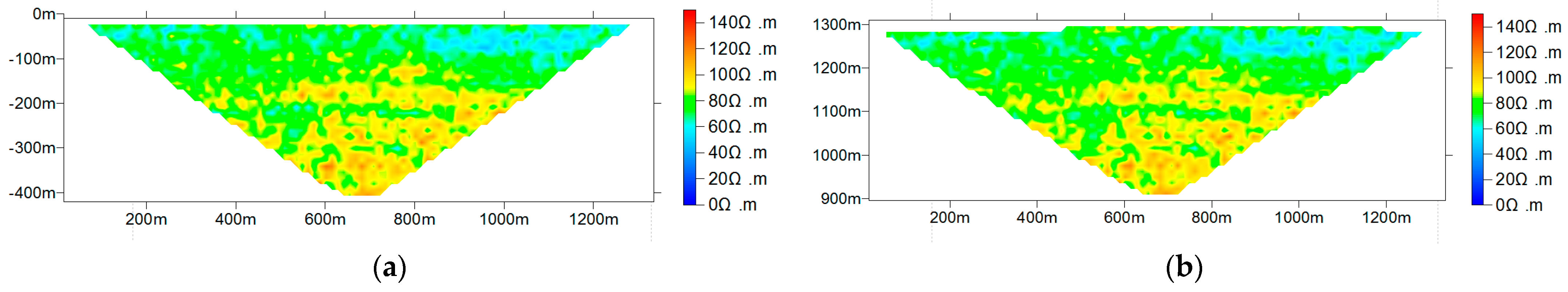
In this fieldwork, the actual elevation and position of each electrode were measured by GPS equipment. A topographic sketch was made in time for particular topographic parts and then organized into the measured topographic profile. During indoor data processing, we use a finite element orthogonal numerical simulation method for the survey area of the geoelectric field to carry out practical topographic correction work. The inversion results along line 2 are illustrated in Figure 4, presenting both pre- and post-topographic correction stages. It is worth noting that in Figure 4a, the vertical coordinate before correction represents the depth, while as shown in Figure 4b and similar electrical profiles in the paper, the vertical coordinate after topographic correction represents the elevation. Although the topography has been incorporated into the inversion process, its differences in the inversion results seem to be merely a displayed topography change on the profile. By comparing the two figures, we can see that the steep slope with obvious topographic changes is near 480 m and 1190 m down the line, which is consistent with the actual geological conditions, indicating that the correction makes the real topographic situation displayed better.

3.3. Interpretation of ERT Data

Compared with conventional electrical data interpretation, time-lapse electrical interpretation focuses on comparing the differences between electrical data at different times. It analyzes the change rule of the electrical properties of the coal strata caused by coal seam mining by comparing the differences in the electrical resistivity of the data from multiple detections. At the same time, in this study, referring to the past research experience and the application experience in the actual experiment, this paper adopts the Quasi-Newton method inversion [25]. Because the Quasi-Newton method only needs the gradient information of the objective function and does not need to calculate the sensitivity matrix explicitly, the number of forward simulations required in each inversion iteration is less. So, it has the advantages of higher efficiency and faster inversion calculation in the iterative process.

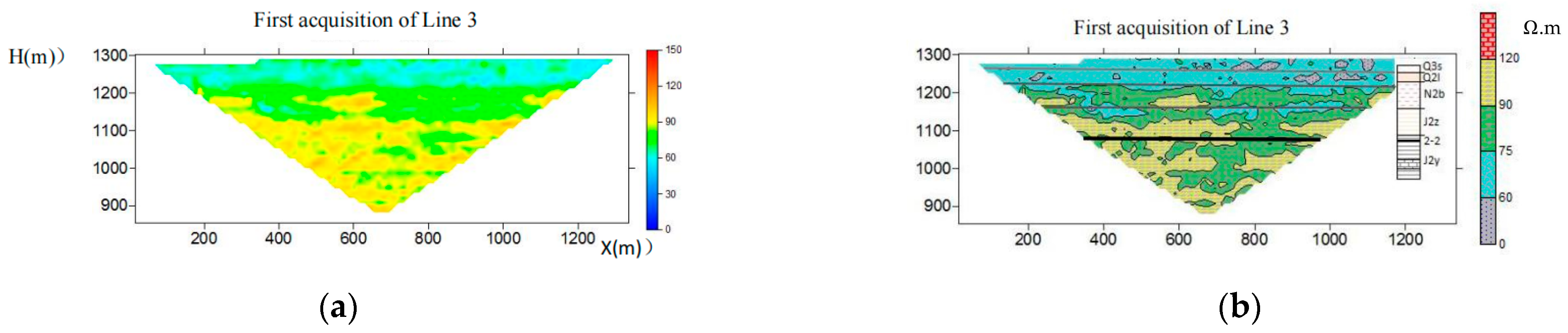
Figure 5a shows the inversion results of the first exploration data of the south flank of the Ningtiaota coal mine’s line 3, and Figure 5b shows the interpretation of the line 3 exploration. There are four main electrical layers developed in the detection area. As seen in the legend in Figure 5b, the main resistivity of the surface sandy soil layer ranges from 35 to 75 Ω.m, while the subsurface loose soil aquifer and the bedrock weathering zone ranges from 75 to 90 Ω.m, and the coal seam overlying the top plate sandstone layer ranges from 90 to 120 Ω.m. Furthermore, the main resistivity of the 2-2 coal seam and its bottom rock layer are higher, and it is worth noting that because 4 m thickness coal seam is determined by previous geological data, it may not be distinguished on the profile.

The first layer is the surface sandy soil layer (Q3s), whose electrical properties are not very uniform, and the resistivity on the right side of the line is generally lower and the low-resistance area increases, which indicates that the water content on the right side of the surface sandy soil layer at the line is relatively strong. The second layer is the subsurface loose soil aquifer (phreatic layer Q2l) and the bedrock weathering zone (N2b), with the overall resistivity becoming slightly higher, and the distribution of this section of the layer is subsurface aquifers and bedrock weathering zone aquifers, presenting low but not uniform resistivity, the local sporadic distribution of some high-resistance areas, and the overall performance of a certain degree of water bearing. The third layer is the coal seam overlying the top plate sandstone layer (J2z and J2y). The distribution of resistivity is also uneven, the overall resistivity becomes high with high and low resistance fluctuations, and lateral continuity is not good because the low-resistivity layer is the top plate sandstone aquifer. The fourth layer is the 2-2 coal seam and its bottom rock layer (J2y), which have high resistivity and poor water content.

In order to make full use of multiple survey line data in the research area, 3D visualization software of electrical data (ED3D V1.1) is developed according to the characteristics of electrical field distribution in this work, and the final results of each survey line are visualized by this software. The visual stereoscopic full view of the four lines of the second test on the south wing of the Ningtiaota mine is shown in Figure 6.

The visualized 3D data body may be used for data extraction in any direction. In the process of interpretation, the vertical and horizontal profiles were combined and verified to repeatedly compare, check, modify, and confirm the data of the district in an all-around way and to ensure that the interpretation results are correct and reliable.

4. Results and Discussion

4.1. Electrical Profile Characteristics of Overlying Strata in Coal Seam Mining

Line 2 is located within the S12002 working face and is directly affected by the working face mining. Figure 7 shows the apparent resistivity profile obtained from the processing of the four times electrical data in line 2.

The electrical profile of the pre-mining period in line 2 is shown in Figure 7a,b. The structure of the four electrical layers is evident in the first acquisition of the electrical profile. The overall performance is that the resistivity increases from shallow to deep, the shallow soil layer and the phreatic layer have low resistivity and good water content, the coal bedrock layer is dominated by higher resistivity, and the bedrock weathering zone and the top plate sandstone layer have an uneven distribution of low resistance and local water content.

The electrical profiles of the in-mining period in line 2 are shown in Figure 7c–f. On the side of the cutting eye of the working face where the coal seam has been mined, the overlying soil and rock layers are obviously affected by mining, the resistivity of the soil and rock aquifers rises to different degrees, the water content deteriorates, and the resistivity of the electrical layer increases in fluctuation, which is more obvious in a particular range near the mining location.

The electrical profile of the post-mining period in line 2 is shown in Figure 7g,h. The electrical structure of each aquifer is similar to that before mining, which indicates that after the mining of the coal seam, the structure of overlying soil and rock layers shows a slow recovery process over time, and the resistivity of local layers in the weathering zone of bedrock and the top and bottom plates of the coal seam decrease, which indicates that the fissure zones formed by damage to overlying rocks of the mined coal seam have not developed into the weathering zone aquifer and that mining makes the water-bearing nature of the coal seam and the bottom plate increase.

4.2. Characteristics of Electrical Changes in the Overlying Aquifer for Coal Seam Mining

Using the data body formed by the monitoring data of four parallel lines in the study area, the resistivity data of different periods of each major aquifer were extracted along the layers, and their changing rules of electrical properties (water content) with the influence of mining were compared and analyzed.

4.2.1. Analysis of the Sandy Soil Layer

Figure 8 is the electrical slice of the surface sand soil layer affected by mining, and its depth is about 10 m.

The surface of the survey area has ups and downs, the composition and thickness of the exposed layer have some changes, and the shallow sand soil layer is dry in the sand-dominated uplift part. The clay in the flat and low-lying parts generally accounts for a large proportion of vegetation development, and the water content is relatively good. As we can see in the first acquisition in Figure 8, before mining (Figure 8a), the electrical properties of the surface sandy soil layer are not uniform, the resistivity of the western part of the survey area is relatively low, and there is a piece of area in the middle southwest with obvious low-resistance characteristics, and the resistivity in the middle east has become higher, with sporadic distribution of high-resistance and low-resistance areas. For the in-mining period (Figure 8b,c), with the advancement of the working face from the south to the north, the resistivity changes, the resistivity of the original low-resistance area of the mined area increases, and the resistivity of the high-resistance area becomes lower. The resistivity near the mining location shows a fluctuating increase phenomenon. The fourth acquisition (Figure 8d) is carried out for about 8 months after the mining of coal seams in the survey area, and the distribution of resistivity in the detection area becomes more uniform at this time, with mainly medium–low resistance (40~70 Ω.m). It shows that mining deforms the sand soil near the mining zone and develops fissures, so the original dry and knotted sand soil is loosened. The resistivity is lowered, the original wet sand soil locally develops fissures, and the resistivity rises due to the influence of mining. The water content of the sand soil layer becomes better and more uniform in general after mining.

4.2.2. Analysis of the Phreatic Layer

The water level of the phreatic layer in the exploration area is about 40 m deep and mainly comprises the sandy soil layer and clay layer. Figure 9 shows the electrical data visual resistivity of the phreatic layer along the layer slice, which was performed four times. Before mining (Figure 9a), the phreatic layer’s visual resistivity was low to medium resistance, and the distribution was relatively uniform, which indicates that the phreatic layer had better and more uniform water content. During the period of mining (Figure 9b,c), the mining causes local groundwater seepage and loss, and the visual resistivity is higher. The resistivity increases more obviously in the zone of influence (about 200 m range before and after) of the mining position. In the post-mining period (Figure 9d), after a period of stability, the resistivity of the phreatic layer becomes low and the uniformity is relatively good, indicating that the water richness of the underground diving layer has recovered to the pre-mining level.

4.2.3. Analysis of the Roof Sandstone Aquifer

The roof sandstone layer in the Zhiluo Formation under the weathering zone of bedrock is selected for analysis. Figure 10 shows the electrical slices of the sandstone aquifer affected by mining. Before mining (Figure 10a), resistivity was relatively high in the western part of the survey area, which is related to the fact that the S12003 working face was mined. The middle and eastern parts of the area are distributed intermittently with medium resistance and low resistance zones, indicating that the roof of the coal seam is unevenly water bearing before mining and has a certain water-rich nature. In the period of mining (Figure 10b,c), due to the influence of mining, the electrical resistivity of the roof aquifer in the mining-affected zone significantly increases, indicating that mining causes damage to the overlying rock, crack development, roof water infiltration, and decreased water content. The detection interval is longer after mining, the range of the detection is no longer under the influence of mining, and the resistivity of this top plate aquifer becomes lower and more uniform (Figure 10d), indicating that at this time, the aquifer is recovering its water-rich nature, and it is even better.

4.2.4. Analysis of the Coal Seam

Figure 11 shows the electrical slice of the 2-2 coal seam affected by mining. Before mining (Figure 11a), the western part of the survey area has some medium resistance areas due to the mining of the S12003 working face, and the middle east coal seam shows high resistance, which indicates that the coal seam in the middle east of the unmined area is dry and does not contain water. In the mining period (Figure 11b,c), the impact of mining makes the resistivity of the coal seam locally decrease, the resistivity is distributed in the middle and high resistance, and the resistivity obviously decreases near the mining position. After mining (Figure 11d), the resistivity of the coal seam generally decreases to medium resistance, indicating that the water from the overlying aquifer seeps down to the goaf, making the coal seam unevenly water bearing, but the water bearing is not strong and is just local weak water bearing. The slice analysis of the bottom plate of the coal seam of the after-mining data body shows that the bottom plate of the coal seam has a localized distribution of water bearing or weak water bearing, which is stronger than that of the water bearing in the coal seam, indicating that the coal seam is filled with water within a certain depth of the subducting bottom plate after mining.

4.3. Analysis of Changes of In-Mining Impacts of Overlying Aquifers for Coal Seam Mining

By adopting data from different observations of the S12002 working face in the south flank of the Ningtiaota mine, the second line located in the middle of the working face was selected. The difference inversion of the dynamic variation of electrical parameters between in-mining and pre-mining and post-mining and in-mining is carried out to reveal the variation law of water-bearing properties in complex rock affected by mining.

By taking the first exploration data before mining of the measuring line 2 as the background value and the difference inversion with the third exploration data in-mining and calculating and obtaining the change amount and change rate of two observation data, the location of the third acquisition was about 800 m north of the survey line.

Figure 12 shows the resistivity change cloud map (Figure 12a) and its interpretation diagram (Figure 12b) obtained by difference inversion. The resistivity changes during and before mining are distributed in the range of −65~55 Ω.m, and ±20 Ω.m is used as the classification criterion for the resistivity change. The figure shows that the roof resistivity increases significantly at about 200 m before and after the mining position of the working face. According to the resistivity distribution in this area, the roof failure electrical zonation can be roughly circled (the height of the fracture zone is about 70–90 m), as shown in Figure 12.

Figure 13 is a cloud map (Figure 13a), and its interpretation (Figure 13b) of the resistivity change rate obtained from the difference inversion between the in-mining and the pre-mining. The resistivity change rate of the in-mining and the pre-mining in the survey line 2 is mainly distributed in the range of −0.9~+0.5. Based on the distribution of the detection data with hydrogeological data of the detection area and the temporal and spatial state affected by mining, ±0.15 was determined as a major criterion for the coloring of the resistivity change rating. It shows that there is a water loss zone with a maximum height of about 90 m in the roof of the coal seam before and after the mining line, and the lower part of the zone is a strong water loss zone (roof damage zone) with a resistivity change rate of more than 15% (below the red line). Upward, there is a water loss fissure zone with a resistivity change rate of 0~15% (between the red line and the yellow line).

It also shows that there are areas of elevated resistivity distributed in the weathered zone of bedrock and loose layers in the upper part of the mined area; there are also areas with increased resistivity, suggesting that mining has certain short-term water loss effects on them.

4.4. Analysis of Changes in Post-Mining Recovery of Overlying Aquifers for Coal Mining

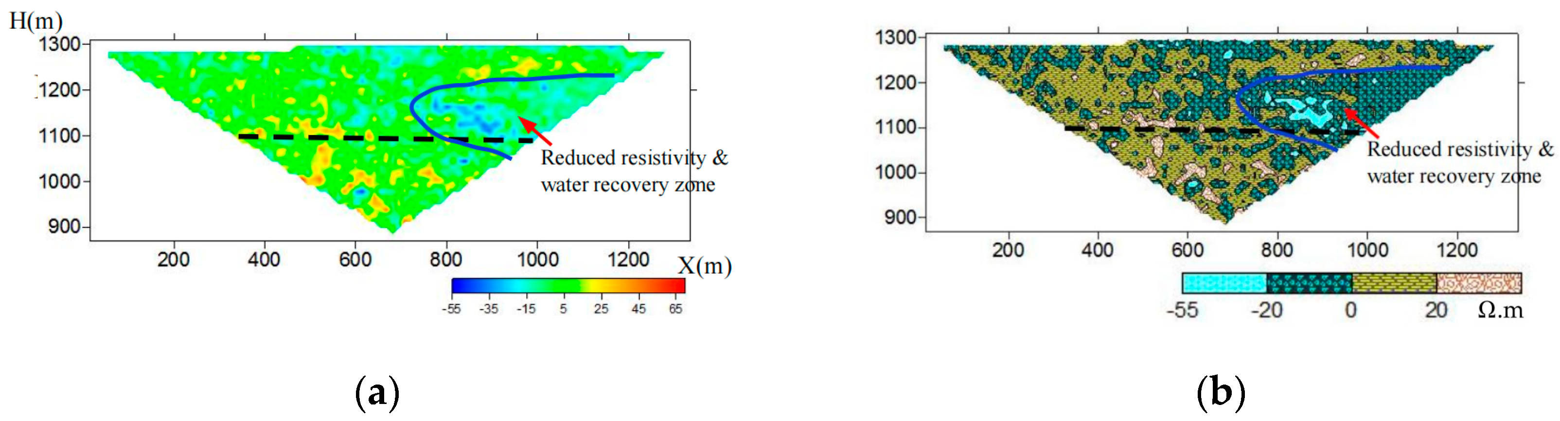
The third acquisition of data from the south flank survey line 2 of the Ningtiaota mine was used as the background value, and the post-mining exploration data were used to perform a difference inversion to find the amount and rate of change in the two observations.

Figure 14 is the survey line 2 of post-mining and in-mining in the third data to find the number of resistivity differences in the plotting of cloud diagrams (Figure 14a) and explanations (Figure 14b). The resistivity changes of post-mining and in-mining are distributed in the range of −55~70 Ω.m to ± 20 Ω.m. As the resistivity changes in grading coloring, resistivity changes at this time reflect the changes from in-mining to post-mining in the last 8 months. They show that the resistivity of the rock layer at the top and bottom of the coal seam located in the middle to the right side is falling. This area should be the part where the rock layer loses water and the resistivity increases due to the influence of mining. During the test interval, this water-losing area recovers and the resistivity decreases, which is equivalent to the result of the gradual self-recovery of water content in the roof aquifer after mining.

Figure 15 shows the inversion of the resistivity change rate using the data difference between post-mining and in-mining in the third data. The resistivity change rate is mainly distributed in the range of −0.90~+0.55, and ±0.15 is used as the main scale value of resistivity change grading and color assignment. It can be seen that the top and bottom plates of the coal seam on the right side of the survey line show the rewatering zone with the decrease in the resistivity, and the aquifer is mainly restored by the recharge, which is called the ‘Reduced resistivity and water recovery zone’ (blue area). The other parts show an irregularly distributed resistivity change rate of >15% (maroon area) in the water loss fissure zone, a resistivity change rate of 0–15% (yellow area) in the part of the water loss zone, and a resistivity change rate of 0–15% (green area) in the part of the water recovery zone, indicating that the mining damage to the overburden rock after mining has the structural and water content of the recovery. The water loss zones are partly recovered in the yellow zone.

The above studies show that the change rule of the water richness of the overlying soil and rock (aquifer) layer under the influence of coal mining can be revealed by time-lapse electrical method monitoring; however, the following aspects still need attention.

• The work carried out in this paper is mainly aimed at mining areas with shallow coal seams, thin bedrock, scarce water resources, and fragile ecological environments. Due to the consistency and stability of time-lapse multiple acquisitions in geophysical methods, the results of this study may have a certain degree of multiplicity of solutions. In future work, we should strengthen the research and improve the acquisition method and inversion algorithm, adopt the spatio-temporal joint inversion method, and use the monitoring data of the mined area to constrain the data of the unmined area to improve the inversion accuracy of the time-lapse method.
• The data in this research result are closely related to the geological and hydrogeological conditions of the overlying soil and rock layer of the 2-2 coal seam in the research area, as well as the mining technology of the S12003 working face. However, the monitoring technology and regularity understanding of the time-lapse electrical method are universal, and the obtained water richness change rule of the overlying soil and rock layer of the 2-2 coal seam can be borrowed by the other mines with similar geological conditions and mining technology in the south flank of the Ningtiaota mine.
• Due to the large time span of this study, there are seasonal rainfall and other climatic factors that may have a certain impact on the interpretation of the final results. In addition, although the phenomenon of gradual self-recovery of aquifer water content was observed in this study, the mechanism of water resource transportation and ecological restoration still needs to be further studied.
• Although there are still some deficiencies in the research methodology, with the rapid advancement of intelligent and green coal mining in China, the use of time-lapse electrical method monitoring technology to study the changing law of water richness of overlying soil and rock layers will play an increasingly important role.

5. Conclusions

Using the time-lapse electrical method to monitor the water richness of the overlying soil and rock layers in the study area, the characteristics of the overlying soil and rock aquifers in the coal system and the changing rules affected by coal mining were revealed, but there are still many areas that can be improved and explored.

• The overlying soil and rock layers in the exploration area are divided into the surface sandy soil layer, phreatic layer (weathering zone aquifer), roof sandstone aquifer, and coal seam, according to their electrical properties. The resistivity distribution characteristics of each electrical layer are clear, the overall performance is that the resistivity gradually increases from the surface downwards, and the electrical layers are not homogeneous in the localization.
• The soil and rock layers overlying the coal seam mining are obviously affected by mining. Within the influence range of mining, the electrical properties of the surface sandy soil layer have been homogenized, the water content of the original dry sandy soil has been enhanced, and the resistivity of each aquifer underneath has been increased to varying degrees. The fluctuation of the resistivity has been increased, indicating that the aquifer’s water content has become poorer.
• After mining and stabilizing for a period of time, the resistivity of the phreatic layer and the overburdened roof aquifer (above the water-conducting fissure zone) become lower and the uniformity becomes relatively better, indicating that the aquifer that has been damaged by mining could be restored to the pre-mining level relatively quick and that there is a certain degree of water accumulation in the goaf and its bottom plate.
• Difference inversion with different simultaneous acquisition data can be used to circle the main influence range of the mining movement using the resistivity change between in-mining and pre-mining to analyze the self-recovery characteristics of the electrical structure of the overburden aquifer using the resistivity change between post-mining and in-mining.

In conclusion, revealing the water richness change rules of the overlying soil and rock before and after mining in the study area can support surface ecological restoration, land reclamation, and water resource protection in the region.

References

- Huang, J.; Yu, H.; Guan, X.; Wang, G.; Guo, R. Accelerated dryland expansion under climate change. Nat. Clim. Change 2016, 6, 166–171. [Google Scholar] [CrossRef]
- Li, C.; Wu, P.; Li, X.; Zhou, T.; Sun, S.; Wang, Y.; Luan, X.; Yu, X. Spatial and temporal evolution of climatic factors and its impacts on potential evapotranspiration in Loess Plateau of Northern Shaanxi, China. Sci. Total Environ. 2017, 589, 165–172. [Google Scholar] [CrossRef] [PubMed]
- Cui, X.; Peng, S.; Lines, L.R.; Zhu, G.; Hu, Z.; Cui, F. Understanding the Capability of an Ecosystem Nature-Restoration in Coal Mined Area. Sci. Rep. 2019, 9, 19690. [Google Scholar] [CrossRef] [PubMed]
- Binley, A.; Hubbard, S.S.; Huisman, J.A.; Revil, A.; Robinson, D.A.; Singha, K.; Slater, L.D. The emergence of hydrogeophysics for improved understanding of subsurface processes over multiple scales. Water Resour. Res. 2015, 51, 3837–3866. [Google Scholar] [CrossRef] [PubMed]
- Du, W.; Peng, S. An application of 4D seismic monitoring technique to modern coal mining. Geophys. Prospect. 2017, 65, 823–839. [Google Scholar] [CrossRef]
- Zou, C.; Zhang, S.; Jiang, X.; Chen, F. Monitoring and characterization of water infiltration in soil unsaturated zone through an integrated geophysical approach. CATENA 2023, 230, 107243. [Google Scholar] [CrossRef]
- Bai, L.; Li, J.; Zeng, Z. Numerical Simulation of Hot Dry Rock Fracture Monitoring by Time-Lapse Magnetotelluric Method. Energies 2022, 15, 7203. [Google Scholar] [CrossRef]
- Ibraheem, I.M.; Tezkan, B.; Bergers, R. Integrated Interpretation of Magnetic and ERT Data to Characterize a Landfill in the North-West of Cologne, Germany. Pure Appl. Geophys. 2021, 178, 2127–2148. [Google Scholar] [CrossRef]
- Ibraheem, I.; Tezkan, B.; Bergers, R. Imaging of a Waste Deposit Site Near Cologne City, Germany Using Magnetic and ERT Methods. In Proceedings of the 25th European Meeting of Environmental and Engineering Geophysics, The Hague, The Netherlands, 8–12 September 2019; Volume 2019, pp. 1–5. [Google Scholar]
- Day, B.; Lachhab, A. Aquifer heterogeneity by mean of ert and bring logs: A case study in peer, susquehanna university. In Abstracts with Programs-Geological Society of America; Society of America: Portland, OH, USA, 2021. [Google Scholar]
- Jodry, C.; Lopes, S.P.; Fargier, Y.; Sanchez, M.; Côte, P. 2d-ert monitoring of soil moisture seasonal behavior in a river levee: A case study. J. Appl. Geophys. 2019, 167, 140–151. [Google Scholar] [CrossRef]
- Cao, Q.; Song, X.; Wu, H.; Gao, L.; Liu, F.; Yang, S.; Zhang, G. Mapping the response of volumetric soil water content to an intense rainfall event at the field scale using GPR. J. Hydrol. 2020, 583, 124605. [Google Scholar] [CrossRef]
- Koestel, J.; Kenna, A.; Javaux, M.; Binley, A.; Verbeeck, H. Quantitative imaging of solute transport in an unsaturated and undisturbed soil monolith with 3-d ert and tdr. Water Resour. Res. 2008, 44, W12411. [Google Scholar] [CrossRef]
- Yu, Y.; Weihermüller, L.; Klotzsche, A.; Lärm, L.; Vereecken, H.; Huisman, J.A. Huisman, Sequential and coupled inversion of horizontal borehole ground penetrating radar data to estimate soil hydraulic properties at the field scale. J. Hydrol. 2021, 596, 126010. [Google Scholar] [CrossRef]
- Blazevic, L.A.; Bodet, L.; Pasquet, S.; Linde, N.; Jougnot, D.; Longuevergne, L. Time-lapse seismic and electrical monitoring of the vadose zone during A controlled infiltration experiment at the Ploemeur hydrological observatory, France. Water 2020, 12, 1230. [Google Scholar] [CrossRef]
- Travelletti, J.; Sailhac, P.; Malet, J.P.; Grandjean, G.; Ponton, J. Hydrological response of weathered clay-shale slopes: Water infiltration monitoring with time-lapse electrical resistivity tomography. Hydrol. Process. 2012, 26, 2106–2119. [Google Scholar] [CrossRef]
- Tesfaldet, Y.T.; Puttiwongrak, A. Seasonal groundwater recharge characterization using time-lapse electrical resistivity tomography in the Thepkasattri watershed on Phuket Island, Thailand. Hydrology 2019, 6, 36. [Google Scholar] [CrossRef]
- Chambers, J.E.; Gunn, D.A.; Wilkinson, P.B.; Meldrum, P.I.; Haslam, E.; Holyoake, S.; Kirkham, M.; Kuras, O.; Merritt, A.; Wragg, J. 4D electrical resistivity tomography monitoring of soil moisture dynamics in an operational railway embankment. Near Surf. Geophys. 2014, 12, 61–72. [Google Scholar] [CrossRef]
- Xu, C.; Zhang, J. Application of time-lapse high-density resistivity method in non-destructive detection for hidden dangers in dikes. Geotech. Investig. Surv. 2023, 51, 73–78. [Google Scholar]
- Lu, J.; Wang, B.; Li, D.; Duan, J. Application of mine-used resistivity monitoring system in working face water disaster control. Coal Geol. Explor. 2022, 50, 36–44. [Google Scholar] [CrossRef]
- Li, F.; Cheng, J.; Chen, S.; Kang, Q.; Li, G.; Liu, D. Fine detection of overburden strata based on time lapse high density resistivity method. J. Min. Sci. Technol. 2019, 4, 1–7. [Google Scholar] [CrossRef]
- Chang, P.Y.; Puntu, J.M.; Lin, D.J.; Yao, H.J.; Chang, L.C.; Chen, K.H.; Lu, W.J.; Lai, T.H.; Doyoro, Y.G. Using time-lapse resistivity imaging methods to quantitatively evaluate the potential of groundwater reservoirs. Water 2022, 14, 420. [Google Scholar] [CrossRef]
- Chambers, J.E.; Meldrum, P.I.; Wilkinson, P.B.; Ward, W.; Jackson, C.; Matthews, B.; Joel, P.; Kuras, O.; Bai, L.; Uhlemann, S.; et al. Spatial monitoring of groundwater drawdown and rebound associated with quarrydewatering using automated time-lapse electrical resistivity tomography and distribution guided clustering. Eng. Geol. 2015, 193, 412–420. [Google Scholar] [CrossRef]
- Meyerhoff, S.B.; Maxwell, R.M.; Revil, A.; Martin, J.B.; Karaoulis, M.; Graham, W.D. Characterization of groundwater and surface water mixing in a semiconfined karst aquifer using time-lapse electrical resistivity tomography. Water Resour. Res. 2014, 50, 2566–2585. [Google Scholar] [CrossRef]
- Ibraheem, I.M.; Bergers, R.; Tezkan, B. Archaeogeophysical exploration in Neuss-Norf, Germany using electrical resistivity tomography and magnetic data. Near Surf. Geophys. 2021, 19, 603–623. [Google Scholar] [CrossRef]
Figure 1.
Survey lines for the working face in the research area.
Figure 2.
Acquisition time of the time-lapse electrical method.
Figure 3.
Comparison of data before and after smoothing.
Figure 4.
Electrical profiles of the second acquisition in line 2: (a) before topography correction; (b) after topography correction.
Figure 5.
First survey inversion result along line 3 on the south flank of the Ningtiaota mine: (a) line 3 second data acquisition resistivity distribution; (b) line 3 second data acquisition interpretation diagram of the electrical structure layer.
Figure 6.
Stereoscopic full view of the second acquisition data of the Ningtiaota mine.
Figure 7.
Electrical profiles of the four acquisitions in line 2: (a), (c), (e), and (g), respectively, represent the resistivity profile for the first (pre-mining), the second (in-mining 1), the third (in-mining 2), and the fourth (post-mining) data acquisition; (b), (d), (f), and (h), respectively, represent the interpretation diagram of the electrical structure layer for the first (pre-mining), the second (in-mining 1), the third (in-mining 2), and the fourth (post-mining) data acquisition.
Figure 8.
Comparison of electrical changes in the surface sandy soil layer affected by mining: (a) resistivity profile for the first (pre-mining) data acquisition; (b) resistivity profile for the second (in-mining 1) data acquisition; (c) resistivity profile for the third (in-mining 2) data acquisition; (d) resistivity profile for the 4th (post-mining) data acquisition.
Figure 9.
Electrical slices of the phreatic layer from four acquisitions: (a) resistivity profile for the first (pre-mining) data acquisition; (b) resistivity profile for the second (in-mining 1) data acquisition; (c) resistivity profile for the third (in-mining 2) data acquisition; (d) resistivity profile for the 4th (post-mining) data acquisition.
Figure 10.
Electrical slices of the top plate aquifer from four acquisitions: (a) resistivity profile for the first (pre-mining) data acquisition; (b) resistivity profile for the second (in-mining 1) data acquisition; (c) resistivity profile for the third (in-mining 2) data acquisition; (d) resistivity profile for the 4th (post-mining) data acquisition.
Figure 11.
Electrical slices of coal seam from four acquisitions: (a) resistivity profile for the first (pre-mining) data acquisition; (b) resistivity profile for the second (in-mining 1) data acquisition; (c) resistivity profile for the third (in-mining 2) data acquisition; (d) resistivity profile for the 4th (post-mining) data acquisition.
Figure 12.
Amount of resistivity change by difference inversion between in-mining and pre-mining for line 2: (a) resistivity change cloud map; (b) electrical structure layer interpretation diagram.
Figure 13.
Rate of resistivity change by difference inversion between in-mining and pre-mining for line 2: (a) resistivity change cloud map; (b) electrical structure layer interpretation diagram.
Figure 14.
Amount of resistivity change by difference inversion between post-mining and in-mining for line 2: (a) resistivity change cloud map; (b) electrical structure layer interpretation diagram.
Figure 15.
Rate of resistivity change by difference inversion between post-mining and in-mining for line 2: (a) resistivity change cloud map; (b) electrical structure layer interpretation diagram.
Disclaimer/Publisher’s Note: The statements, opinions and data contained in all publications are solely those of the individual author(s) and contributor(s) and not of MDPI and/or the editor(s). MDPI and/or the editor(s) disclaim responsibility for any injury to people or property resulting from any ideas, methods, instructions or products referred to in the content. |
© 2024 by the authors. Licensee MDPI, Basel, Switzerland. This article is an open access article distributed under the terms and conditions of the Creative Commons Attribution (CC BY) license (https://creativecommons.org/licenses/by/4.0/).
Share and Cite
MDPI and ACS Style
Zhu, C.; Zhu, G.; Gong, Y.; Zhang, L. Research on the Monitoring of Overlying Aquifer Water Richness in Coal Mining by the Time-Lapse Electrical Method. Energies 2024, 17, 1946. https://doi.org/10.3390/en17081946
AMA Style
Zhu C, Zhu G, Gong Y, Zhang L. Research on the Monitoring of Overlying Aquifer Water Richness in Coal Mining by the Time-Lapse Electrical Method. Energies. 2024; 17(8):1946. https://doi.org/10.3390/en17081946
Chicago/Turabian StyleZhu, Chenyang, Guowei Zhu, Yufei Gong, and Lei Zhang. 2024. "Research on the Monitoring of Overlying Aquifer Water Richness in Coal Mining by the Time-Lapse Electrical Method" Energies 17, no. 8: 1946. https://doi.org/10.3390/en17081946
Note that from the first issue of 2016, this journal uses article numbers instead of page numbers. See further details here.