

Experimental Identification of a Coupled-Circuit Model for the Digital Twin of a Wound-Rotor Induction Machine

Laboratory of Electrical Engineering, Power Electronics and Industrial Control (LEEPEIC), Department of Electrical and Computer Engineering, Laval University, 1065 Avenue de la Médecine, Quebec, QC G1V 0A6, Canada
*
Author to whom correspondence should be addressed.
Energies 2024, 17(8), 1948; https://doi.org/10.3390/en17081948
Submission received: 22 January 2024
/
Revised: 10 March 2024
/
Accepted: 12 April 2024
/
Published: 19 April 2024
(This article belongs to the Special Issue Advanced Topologies and Control Strategies in Electric Machines and Drives)
Abstract
:The development of monitoring and diagnostic methods for electrical machines requires the use of transient models capable of operating in real time and producing signal signatures with high precision. In this context, coupled-circuit models offer numerous advantages due to their speed of execution and accuracy. They have been successfully employed to create real-time digital twins of electrical machines. The main challenge of this modeling method lies in the preparation of the model, which involves numerous preliminary calculations and takes time to identify all its parameters. This is particularly due to the variation in inductances based on the rotor position. To determine these inductance values with great precision, the classical approach involves using finite-element field calculation software. However, the computation time quickly becomes an issue due to the large number of values to calculate and simulations to perform. This article introduces an innovative experimental approach to identify a coupled-circuit model and develop a digital twin of a wound-rotor induction machine. This method relies solely on simple electrical measurements and tests conducted at extremely low rotation speeds (1 rpm) to obtain inductance variations as a function of the rotor position. By employing this technique, the need for analytical models or finite-element field calculation simulations, which typically require precise knowledge of the machine’s geometry and materials, is circumvented. The measurement processing employs optimization methods to extract the inductances as a function of the rotor position, which are then used as input data for the coupled-circuit model. The final parameters are specific to each machine and replicate all its manufacturing imperfections such as eccentricity and geometric or winding defects. This experimental identification method significantly enhances the model’s accuracy and reduces the usually required preliminary calculation time in a finite-element-based identification process.
1. Introduction
Wound-rotor induction machines, commonly referred to as slip-ring induction motors, present an enticing solution for applications demanding robust starting torque and precise variable speed control. Their versatility extends across a wide array of industrial sectors, encompassing tasks ranging from crushing, grinding, and conveying to elevating. Furthermore, these machines exhibit adaptability in specific power generation domains, such as small hydroelectric plants and small-scale wind turbines. At the forefront of research in this field lies a predominant focus on enhancing condition monitoring methodologies and fault diagnosis techniques for early fault detection [1,2]. The efficacy of these methodologies hinges on a comprehensive understanding of machine behavior under various operational conditions, often necessitating a thorough analysis of data from simulation models and the identification of anomalous signatures [3].
In the realm of machine simulation, the objective is to produce results that accurately reflect the behavior of real-world machines while keeping computational time to a minimum [4]. This is crucial for various reasons, including the optimization of designs, predictive maintenance, and understanding complex system interactions [2,5]. Real-time transient simulations pose significant challenges when very high accuracy is required for voltage and current waveforms, as in the case of signature analysis for diagnostic purposes [6]. To achieve this level of accuracy, researchers and engineers have developed the concept of a digital twin. A digital twin is essentially a virtual replica of a physical machine or system, capturing its characteristics, behavior, and performance in real time or near real time [2,7]. The electromagnetic representation of the machine must be able to reproduce all interactions between the time and space harmonics that are characteristic of the geometry and winding [2]. One notable approach in the development of digital twins for electrical motors is the Multiple Magnetically Coupled Circuits (MMCC) model. This model is particularly renowned for its ability to emulate wound-rotor asynchronous machines with remarkable precision and efficiency. The MMCC model stands out due to its comprehensive consideration of the machine’s geometry and space harmonics [8]. By integrating these factors into its framework, the MMCC model can provide highly accurate simulations of machine behavior under different operating conditions. This level of detail and accuracy makes the MMCC model promising for real-time operation, allowing for dynamic adjustments and monitoring of machine performance [8]. Overall, the development of advanced simulation models like the MMCC model plays a crucial role in advancing various fields, including machine design, optimization, and predictive maintenance. These models enable engineers and researchers to gain deeper insights into machine behavior, leading to more efficient and reliable systems in practice.
However, an important challenge in the practical application of this model lies in the identification of its time-dependent parameters. Indeed, the inductances vary depending on the position of the rotor [8], and their determination requires a very large number of calculations or measurements. This identification process is inherently intricate and often requires other analytical or numerical models to accurately calculate these values. Among the common methods employed for parameter identification are the Winding Functions Method (WFM) [9,10,11] and the utilization of precomputed inductance functions with the finite-element method (FEM) [12]. The WFM involves using mathematical functions to represent the magnetic field distribution within the machine, allowing for the calculation of parameters [2]. On the other hand, employing precomputed inductance functions with the FEM entails utilizing detailed numerical simulations to compute inductance values for different rotor positions [8]. The finite-element method (FEM) is renowned for its versatility and ability to model complex systems with high accuracy [13]. One of its strengths lies in its capability to incorporate detailed geometric effects, such as magnetic leakage flux, which can significantly impact machine performance [7]. However, despite its advantages, implementing the FEM for parameter identification requires comprehensive data on the geometry, materials, and windings of the machine under investigation [8,13]. This necessitates thorough knowledge and detailed characterization of the machine components, which may not always be readily available. Furthermore, the creation and solution of the FEM can be time-consuming and computationally intensive, especially for complex systems. The process involves discretizing the machine geometry into small elements and solving complex equations iteratively to obtain accurate results [8,12,13,14]. As a result, utilizing the FEM for parameter identification may require a considerable investment of time and computational resources, particularly for large-scale or intricate machine designs.
The methodology proposed in [15] represents a notable advancement, as it integrates empirical data with analytical methods to estimate the parameters of a coupled-circuit model. This hybrid approach offers promise for more accurate parameter estimation of induction motors with squirrel-cage rotors. However, a significant challenge arises from the lack of a specialized experimental technique solely focused on measuring inductance variations. Current experimental methods often lack the precision and detail required to match the accuracy achieved through finite-element method (FEM) analysis-based identification. Thus, the method presented in [15] is a promising avenue, even though parameter generation requires some information on motor geometry. This paper presents a revolutionary approach to accurately measure the variation in inductances as a function of the rotor position through experiments conducted at very low speed, similar to standstill tests. By meticulously capturing current and voltage waveforms across different power conditions, advanced analysis and processing techniques are employed to extract the parameters of the machine’s coupled-circuit model utilizing optimization methods. The identified inductance variations are then compared to the finite-element method (FEM) simulations, and the coupled-circuit model simulation is validated through experimental comparisons to demonstrate the very high accuracy of this digital twin.
2. Formulation for the Coupled-Circuit Model
The wound-rotor induction machine is a variant of the asynchronous machine, in which the rotor is equipped with coils and slip rings. This machine offers several advantages over the standard squirrel-cage asynchronous machine, including greater flexibility in terms of speed and torque control [8]. However, modeling a wound-rotor asynchronous machine is complex due to the interactions between the stator and the rotor. The coupled-circuit model is one of the most commonly used methods for modeling the wound-rotor asynchronous machine, especially for the diagnosis and development of digital twins.
Figure 1 illustrates an electrical diagram, which represents the three windings of the rotor (a, b, c) and those of the stator (A, B, C). The angle is the rotation angle of the rotor relative to the stator. In this study, the following assumptions are utilized for constructing the coupled-circuit model [12]:
- The magnetic induction of materials is considered linear, allowing for the neglect of hysteresis and magnetic saturation effects;
- Eddy currents and capacitive effects in winding are negligible;
- Iron losses in magnetic circuits are neglected.
The magnetic flux received at a given circuit from another one depends on the current I flowing in the sender and the magnetic coupling L between the two. The coupling is a function of the rotor angular position .
represents the self-inductance of circuit i and denotes the mutual inductance between circuit i and j. All these inductances vary depending on the rotor position .
It is possible to consolidate all the flux equations describing the electric machine into a single matrix equation.
Using a passive convention, the voltage equation is:
where is the vector of the stator and rotor voltages [V], is the matrix of the stator and rotor resistances [], and is the vector of the stator and rotor currents [A].
As and are functions of time t:
where is the angular velocity in rad/s.
3. Experimental Method for the Measurement of Inductances as a Function of the Rotor Position
3.1. Description of Identification Protocol
This identification method is designed to derive the parameters of a coupled-circuit model for a wound-rotor induction machine (WRIM) based on the rotor position. It uses only standstill tests, which are repeated for a large number of rotor positions. With a sinusoidal power supply, it is possible to use the fundamental electromagnetic equation in a steady state, in phasor, when the rotor is stopped in a given position .
where is the impedance matrix for the rotor position ; is the vector of the voltage phasors, represented as phasors; and is the vector of the current phasors.
Equations (7) and (8) are obtained with the electrical pulsation of the electrical supply.
Equation (8) relates the voltage , resistance R, current , electrical angular frequency , rotor position , and inductance L of the machine. The steps followed are as follows:
- Step 1—Experimental Tests: A series of experiments on the electrical machine are conducted with a 60 Hz sinusoidal voltage supply. The electrical quantities (voltage and current) of all the stator and rotor windings are measured simultaneously to obtain the phasor values. These values are used to extract the circuit parameters from a given rotor position. The set of tests to be carried out is described in more detail in the next paragraphs.
- Step 2— Low-speed Rotation: Considering the dependence of inductances on the rotor position, the rotor is driven to a stable and very low speed of 1 RPM during each test. This approach is based on three key assumptions:
- The electromotive force induced by the rotation of the rotor is considered negligible, thus having no impact on the current and voltage measures.
- The supply frequency (60 Hz) must be significantly higher than the rotation speed (1 Hz). This allows for consideration that the signals over one electrical period remain periodic for the phasor analysis, suggesting constant impedances, equivalent to a standstill rotor test.
- It is important to prevent any significant magnetic saturation that could result from excessive current values.
- Step 3—Data Acquisition: While the rotor is in motion, various waveforms over time can be recorded using an oscilloscope. This includes the voltages and currents flowing through the stator and rotor windings. Additionally, the rotor position is acquired throughout the test.
- Step 4—Data Storage: Each test ends after one complete revolution, which lasts for one minute at a speed of 1 RPM. The collected data are then stored in files and loaded into analysis software such as Matlab.
- Step 5—Processing: The final step involves processing the collected data. The inductance matrix is intended to be computed as a function of the rotor position.
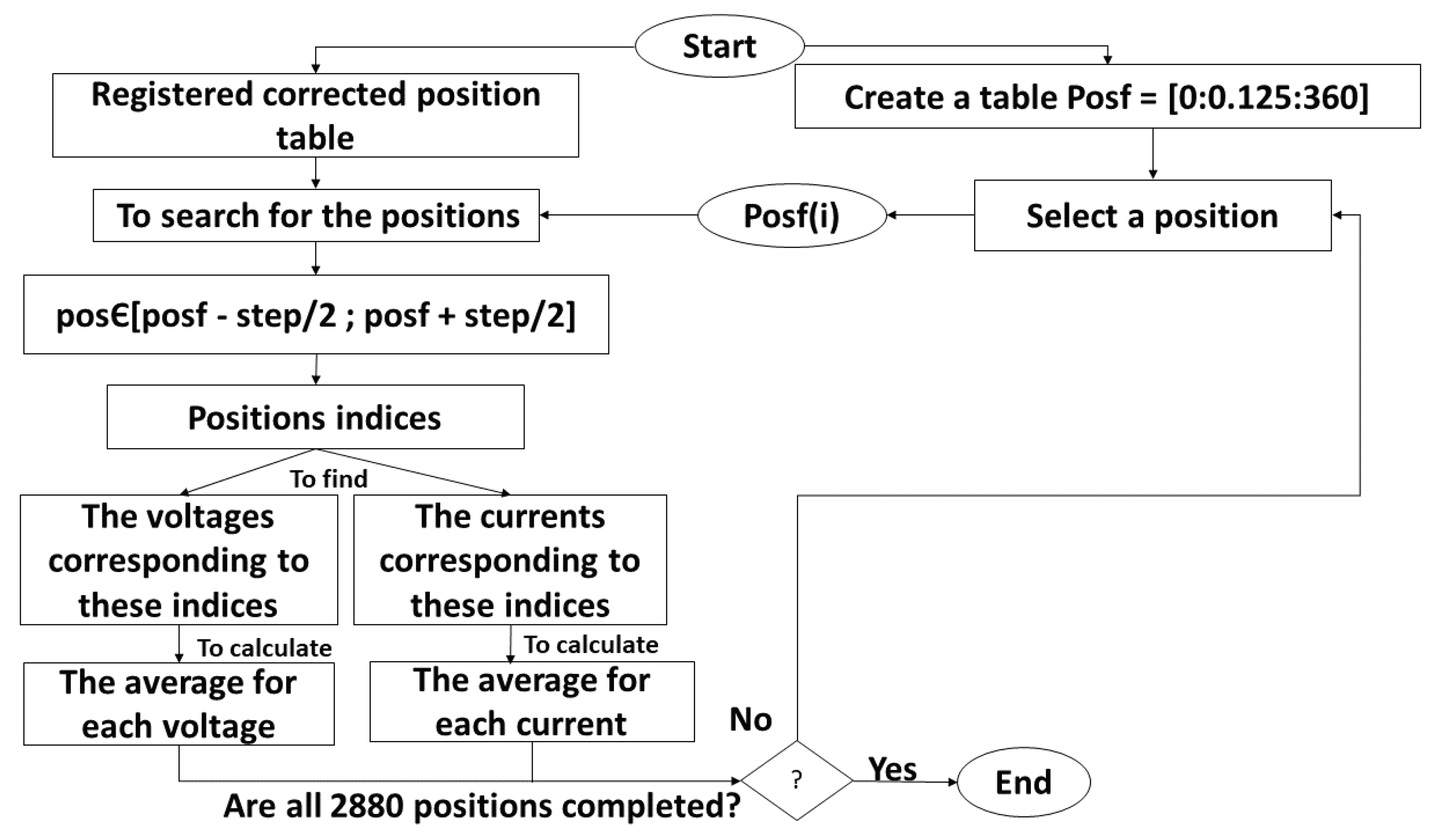
Figure 2 summarizes the procedure for the identification of inductances using the experimental method.
After identifying all parameters, the model performance can be evaluated by comparing the simulated and experimental waveforms. Additionally, the obtained parameters can be compared to those identified through a finite-element field calculation model [8].
3.2. Description of the Wound-Rotor Induction Motor (WRIM)
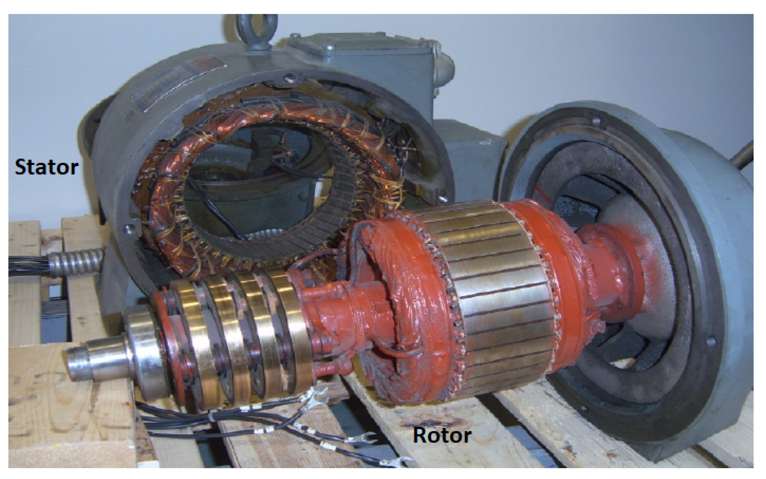
The experiments are conducted on a 2.5 HP wound-rotor induction machine. To validate the measurement method, it is repeated for four identical machines. Appendix A provides further details on the dimensions, winding, and nameplate of this machine. Figure 3 shows a disassembled motor.
This machine has 6 electrical circuits to identify: 3 stator windings and 3 rotor windings (Figure 3). In total, 42 parameters need to be determined for each rotor position. These parameters are as follows:
- The 6 resistances of the windings;
- The 6 self-inductances of the windings;
- The 30 mutual inductances between the windings.
The winding diagram is illustrated in Figure 1. The indices represent the three stator windings, and represent the three rotor windings.
The resistance matrix is diagonal.
represent the resistances of the three stator windings, and represent the resistances of the three rotor windings.
The inductances matrix to be identified for a given rotor position has the following form:
The inductance matrix varies depending on the rotor position. For each position, 36 parameters need to be determined. The machine has 48 slots in the stator, resulting in a slot pitch of 7.8° (360/48). Consequently, a coupled-circuit model was chosen, employing a discrete rotation step of 0.125°. This distribution provides a sufficiently adequate representation of the spatial harmonics [16]. Therefore, there are 2880 discrete positions (360°/0.125°), and each rotor position has a different inductance matrix.
Ensuring the accuracy of representing the spectral content of inductance curves hinges on maintaining a small angle step size. In our investigation of a machine featuring 48 stator slots and 36 rotor slots, we discovered that the fundamental slot generates 144 periods per revolution (LCM(48, 36) = 144). To effectively capture this phenomenon, we opted for 20 points per period, culminating in a total of 2880 positions per revolution.
While it may seem tempting to increase the step size to reduce the computational workload, doing so compromises precision and filters out crucial slot harmonics. Our research, extensively documented in [17], has underscored this effect. Therefore, the approach of using 20 points for each fundamental slot harmonic period is consistently adhered to.
3.3. Test Bench
The power supply comes from a balanced 60 Hz three-phase electrical network. The three-phase network is connected to the motor via an autotransformer, through which the supply voltage can be varied, offering the possibility to adjust the voltage from 0 to 208 volts.
Several oscilloscopes are utilized as waveform acquisition systems, employing differential voltage probes and current clamps.
The main challenge lies in ensuring the perfect synchronization of recordings across multiple oscilloscopes to guarantee the integrity and accuracy of the data. To achieve simultaneous startup of all devices, a common trigger signal is utilized for all acquisition systems.
The rotor position sensor provides a 12-bit signal, which is an analog-to-digital converter with the manufacturing reference AD7245AAN. Ultimately, a signal ranging from −5 to +5 V DC over 360 mechanical degrees of rotation of the machine is obtained. This signal can be captured via a BNC connector, directly connected to an oscilloscope.
The passive convention has been adopted in accordance with the coupled-circuit model equations. Consequently, the direction of the current and the polarity of the voltage for each winding are clearly defined. A common rotor position reference for all tests is essential for accurate results processing.
The decision was made to initialize the rotor position by aligning the axes of the stator winding A and the rotor winding a.
To correctly align the rotor, it is possible to power stator phases B and C in series and connect a voltmeter to the terminals of the rotor phase a. The rotor is moved until the voltage on the voltmeter is zero.
3.4. The Tests and Measurements to Be Carried Out
3.4.1. Measurement of Resistances
In the context of electric machines, the winding resistance has a significant influence on performance. This resistance does not vary with the rotor position.
The classical measurement method involves using a direct current (DC) power source to supply a stationary winding. By measuring the current and applied voltage, one can deduce the value of the internal resistance of the respective winding using Ohm’s law.
3.4.2. Tests for the Identification of Inductances
In total, 13 different tests were performed. During the first six tests, a separate phase was supplied each time with a sinusoidal voltage, providing us with 6 equations with 6 unknowns for each test. Although these six tests are sufficient to define the parameters of the 6 circuits, additional tests were incorporated into the process to characterize the zero-sequence inductance and leakage inductances. Increasing the number of tests improves precision in reproducing varied operating conditions. Throughout the tests, the rotor was driven at 1 RPM while measuring the voltages and currents of the stator and rotor windings, along with the rotor position.
- Test 1: The first phase of the stator, denoted as A, was powered, while the other phases were left open-circuited, as illustrated in Figure 4. This test allows for identifying the first line of the inductance matrix.Figure 4. Test 1 circuit.
![Energies 17 01948 g004]()
- Test 2: The second phase of the stator, denoted as B, was powered, while the other phases were left open-circuited, as illustrated in Figure 5, to identify the second line.Figure 5. Test 2 circuit.
![Energies 17 01948 g005]()
- Test 3: The third phase of the stator, denoted as C, was powered, while the other phases were left open-circuited, as illustrated in Figure 6, to identify the third line.Figure 6. Test 3 circuit.
![Energies 17 01948 g006]()
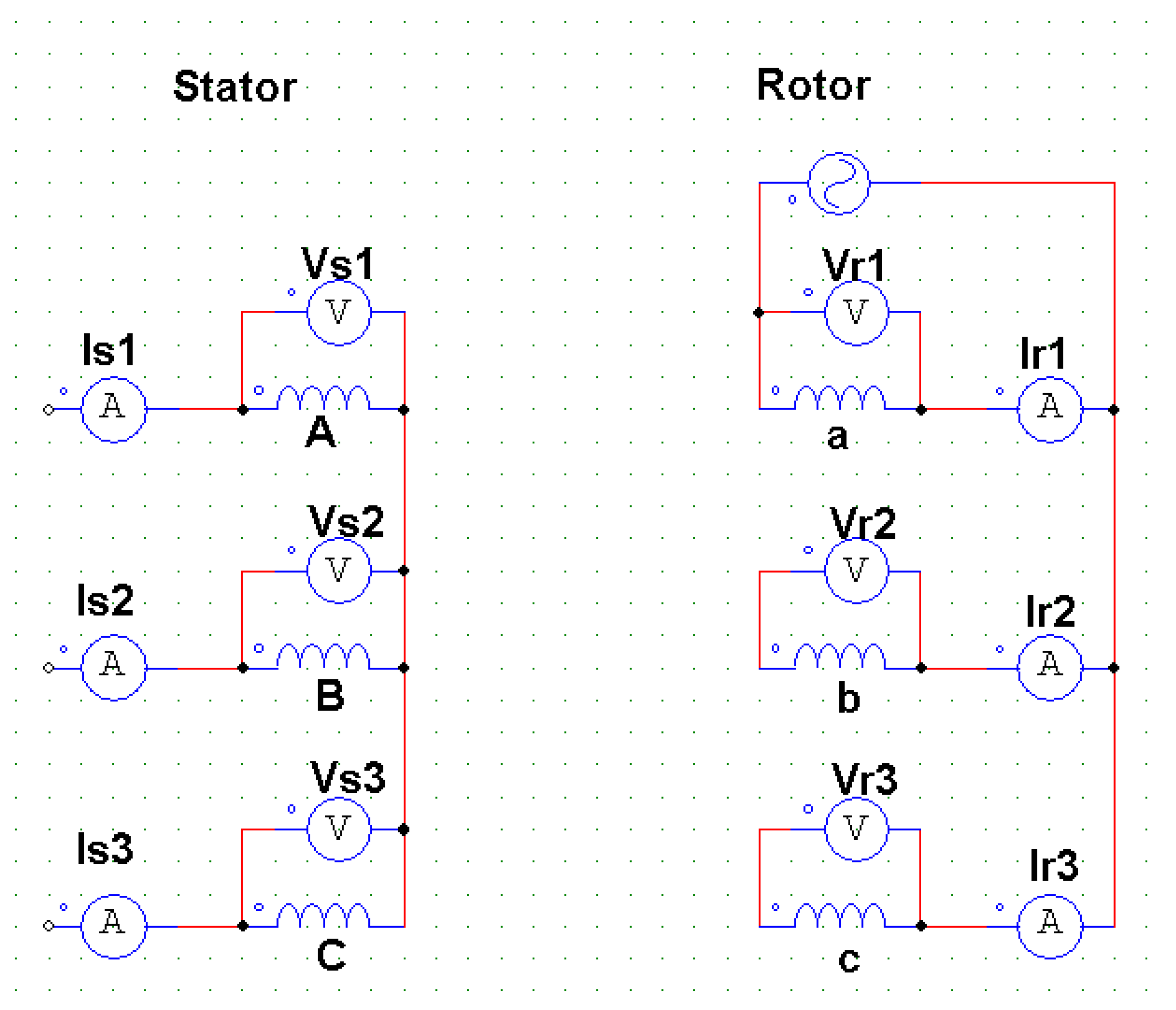
- Test 4: The first phase of the rotor, denoted as a, was powered, while the other phases were left open-circuited, as illustrated in Figure 7, to identify the fourth line.Figure 7. Test 4 circuit.
![Energies 17 01948 g007]()
- Test 5: The second phase of the rotor, denoted as b, was powered, while the other phases were left open-circuited, as illustrated in Figure 8, to identify the fifth line.Figure 8. Test 5 circuit.
![Energies 17 01948 g008]()
- Test 6: The third phase of the rotor, denoted as c, was powered, while the other phases were left open-circuited, as illustrated in Figure 9, to identify the sixth line.Figure 9. Test 6 circuit.
![Energies 17 01948 g009]()
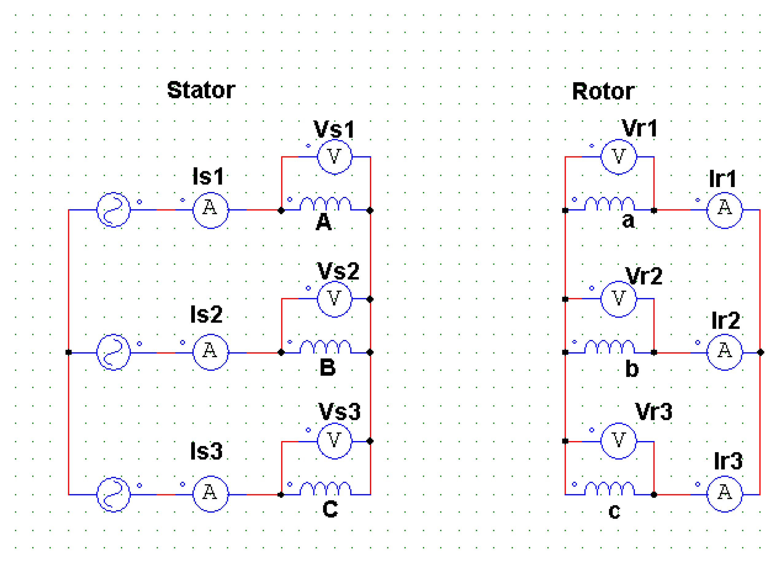
- Test 7: All three phases of the stator, denoted as A, B and C, were powered with a balanced, direct-sequence voltage source, while the star-connected rotor winding was short-circuited, as illustrated in Figure 10. This test highlights the stator-side leakage inductance.Figure 10. Test 7 circuit.
![Energies 17 01948 g010]()
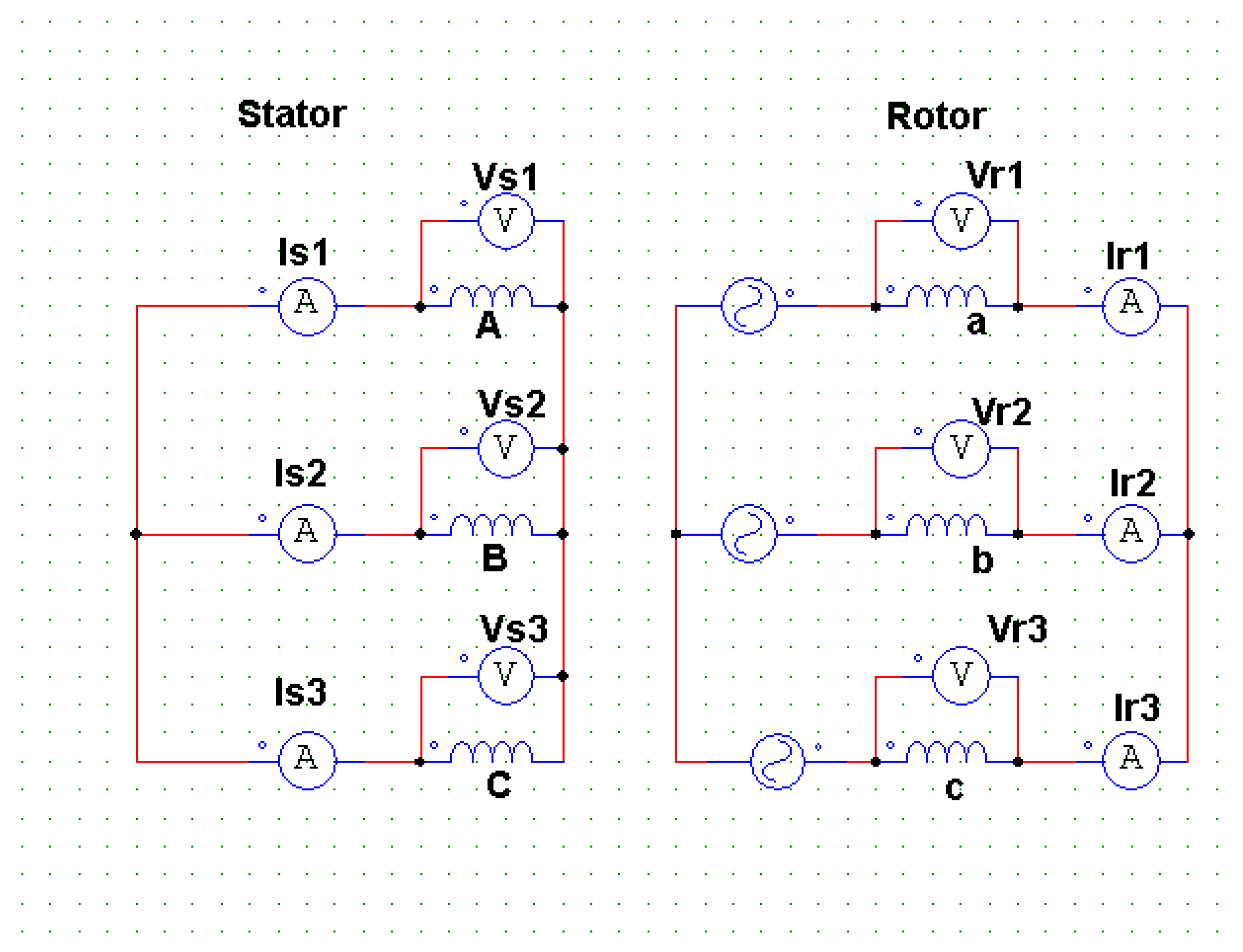
- Test 8: All three phases of the rotor, denoted as a, b and c, were supplied with a balanced, direct-sequence voltage source, while the star-connected stator winding was short-circuited, as illustrated in Figure 11. This test highlights the rotor-side leakage inductance.Figure 11. Test 8 circuit.
![Energies 17 01948 g011]()
- Test 9: Two phases of the rotor, a and b, were supplied, while the other phases were left open-circuited, as illustrated in Figure 12.Figure 12. Test 9 circuit.
![Energies 17 01948 g012]()
- Test 10: Two phases of the stator, A and B, were supplied, while the other phases were left open-circuited, as illustrated in Figure 13.Figure 13. Test 10 circuit.
![Energies 17 01948 g013]()
- Test 11: Two phases of the stator, A and B, were supplied. The first phase of the rotor, a, was short-circuited, while the other phases remained open-circuited, as illustrated in Figure 14.Figure 14. Test 11 circuit.
![Energies 17 01948 g014]()
- Test 12: All three phases of the stator, A, B and C, were supplied with an unbalanced voltage amplitude source in a direct sequence, while the star-connected rotor winding was short-circuited, as illustrated in Figure 15.Figure 15. Test 12 circuit.
![Energies 17 01948 g015]()
- Test 13: The stator phase was connected in series to the voltage power supply, while the rotor winding was left open-circuited, as illustrated in Figure 16. This test highlights the zero-sequence inductance of the machine.Figure 16. Test 13 circuit.
![Energies 17 01948 g016]()


3.5. Experimental Data Processing
A three-step processing method is used to compute the inductances and their variations based on the rotor position. The first step is the computation of the voltage and current phasor values with a Fourier analysis. The second step is the conversion of time-dependent measurements into data, expressed according to discrete angular positions. The third step is an optimization process to extract the inductance values corresponding to each rotor position.
3.5.1. Phasor Computation Using Fourier Analysis
Fourier analysis is used to convert signals into phasors in the frequency domain. The signals recorded by the oscilloscopes may exhibit a significant amount of noise or harmonics, making it challenging to identify the inductances. To address this, only the fundamental frequency of 60 Hz is analyzed, and the magnitude and phase of the fundamental component of each signal in a given rotor position are extracted. Signals captured by oscilloscopes can be disturbed and may not be perfectly sinusoidal, but the use of the phasor method makes the inductance identification method more robust and less sensitive to these disturbances.
3.5.2. Time-Angular Conversion and Angular Position Discretization
The conversion of data measured as a function of time into data expressed as a function of the rotor angle makes it possible to simplify inductance calculation processing. It is also necessary to discretize the position of the rotor with constant intervals to construct the different inductance matrices that will be used by the coupled-circuit model. In this example, the measured values of the steady-state phasors are expressed as a function of 2880 discrete rotor positions before calculating the inductances.
The diagram in Figure 17 summarizes the angular discretization process according to the rotor position.
3.5.3. Calculation of Inductances with an Optimization Procedure
The last step of the processing concerns the calculation of the inductance matrix for each discrete position of the rotor. The least-squares method is utilized, which involves minimizing the mean square error between the voltage phasors calculated with the circuit equations and the measured values by iteratively adjusting the inductance values. For a given rotor position, the inductance values are the variables of the optimization problem, and the least-square error is the function to be minimized. The electrical pulsation and the resistance values are imposed to compute the values of the impedances. The voltages are then calculated using the values of the measured currents, and the sum of the squared errors between the measured voltages and the calculated voltages (refer to Figure 18) is computed. The optimization problem can be solved with the Matlab function fmincon to minimize the error and find the inductance values that best reproduce the behavior of the machine. This process is repeated for the 2880 positions to obtain all inductance matrices. Figure 19 illustrates the procedure for calculating the inductances with the optimization process. To further refine the results, a second optimization can be performed using the calculated inductances as the initial values.
where represents the measured voltage phasors of each test and represents the calculated voltage phasors using the estimated impedances and measured currents.
For each position, the optimization performed between 70 and 83 iterations before reaching the final result and the average execution time is 0.9 s. Considering the 2880 positions, the total time required to identify the inductance matrices is about 29 min. It should be noted that this calculation can be easily parallelized by processing a number of rotor positions with multiple computers. This performance highlights the efficiency of the tool in managing and optimizing inductances.
4. Results
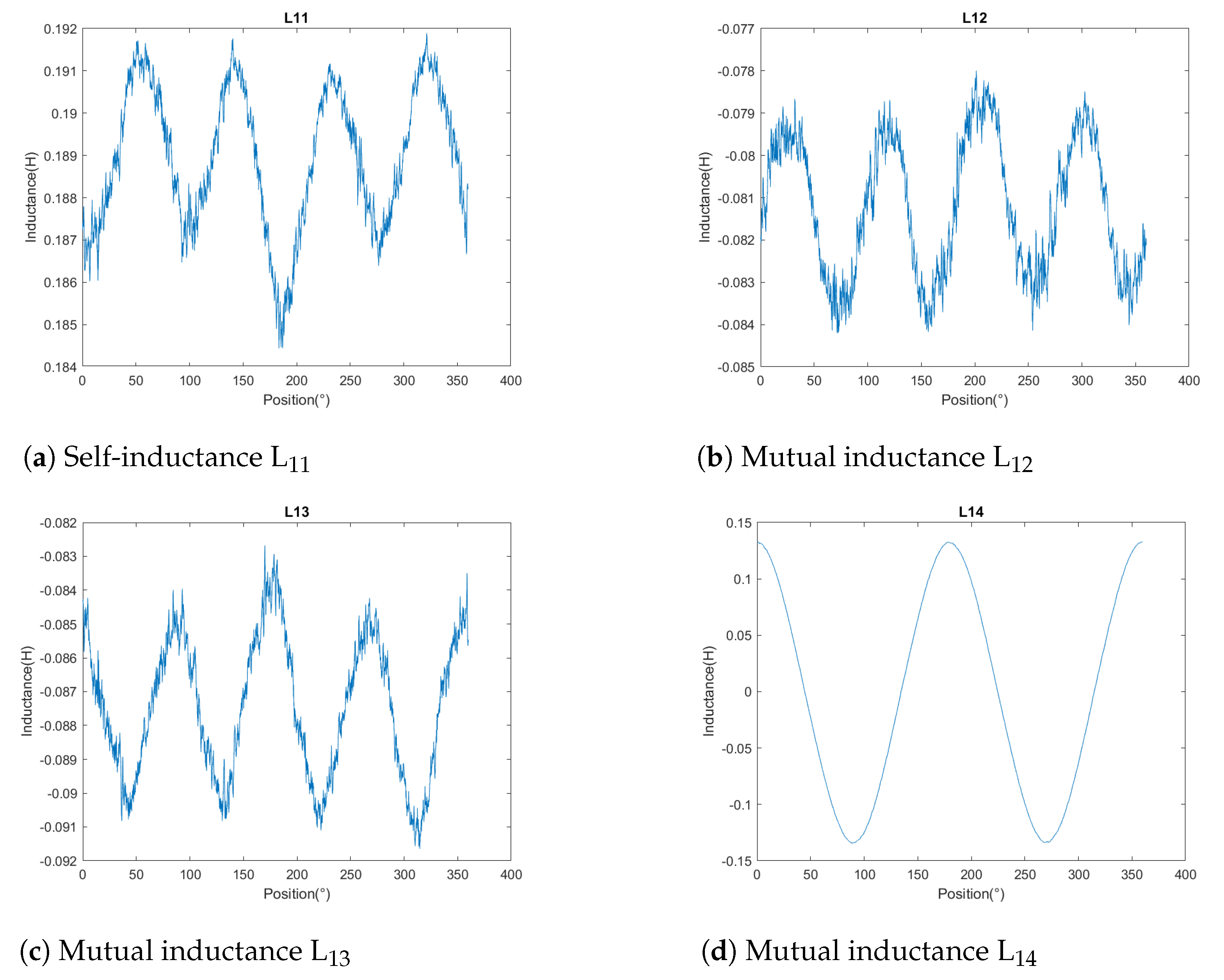
Figure 19a–d depict the various shapes of the inductances measured using this method. Figure 19a illustrates , representing the self-inductance of the first stator phase. Figure 19b shows , indicating the mutual inductance between the first stator phase and the second stator phase. Figure 19c displays , representing the mutual inductance between the first stator phase and the third stator phase. Finally, Figure 19d depicts , illustrating the mutual inductance between the first stator phase and the first rotor phase.
It can be observed that the self-inductances and mutual inductances of the stator are not constant and symmetrical with respect to the rotor position. There are four oscillations per revolution, corresponding to the number of poles on the rotor. The slotting effect is also obvious. Regarding the mutual inductance between the stator and rotor, the profile is strongly sinusoidal, but the slot effect is less obvious.
Error Criterion and Validation
In order to assess the performance of this identification method, the final value of the least mean square error of each test was compared with those obtained from the 2D finite-element analysis-derived inductance matrices [8]. It should be noted that the inductance matrices calculated by the finite-element method (FEM) have been corrected to take into account the coil heads and the effect of rotor slot skewing [8]. Additionally, a comparison was conducted among four copies of identical machines from the same mass production.
Table 1 displays the total relative error of each test with the finite-element method and each motor. The error varies from one test to another. It can be observed that the circuit model with the parameters identified through field calculation has a larger error compared to the measurements for tests 12 and 13. Test 12 involves a voltage imbalance, while test 13 involves a zero-sequence flux when the stator windings are series-connected to the power supply. It can be seen that identification using the experimental method is more efficient than identification based on the finite-element method. Indeed, the penultimate line of the table shows the deviation from the calculation of the finite-element method using a relative error calculated in % with Equation (13). For three motors, the total error is reduced to about 40–50%. It is also evident that there are some differences between the four motors of the same construction, while the finite-element method cannot highlight these differences. Motors and show the largest deviations from motors and .
5. Comparison with Inductances Calculated by the Finite-Element Method
Due to the time-consuming nature of the finite-element method [14] and the periodic geometry of the machine, the study domain was limited to half of the machine [8], assuming perfect symmetry of the geometry and no eccentricity. The angular discretization step for the rotor position was set at 0.125°, resulting in 1440 different positions between 0° and 180°. While this allowed for obtaining 20 points per period of the fundamental slot harmonic in this machine, the computation time exceeded 4.8 h. This issue of computation time with finite-element field calculation software was also highlighted in [13] for another example of ABC model identification. The following figures depict the variations in the inductances over 180 degrees. Here, CAL denotes the inductances obtained by the FEM, while EXP represents the measured inductances using the experimental method.
Figure 20 shows the variation in the self-inductance of the second phase of the stator with respect to the position, and Figure 21 shows the variation in the mutual inductance between the second and third phases of the stator.
The variation in the inductance calculated with FEM is very regular and corresponds to the slotting effect of the rotor and the stator. The number of periods per revolution of this oscillation is obtained by calculating the least common multiple between the number of stator slots (48) and the number of slots in the rotor (36). Here, there are 144 periods, and the amplitude of this oscillation is approximately 0.1 mH for the stator (Figure 20).
Even though the mean values of the measured and calculated inductances are very similar, the experimental result highlights other imperfections of the machine that are not taken into account in the finite-element model. There is an oscillation of four periods per revolution of 0.3 mH, which corresponds to the number of poles. This oscillation is also observed in the self- and mutual inductances of the rotor. This is probably due to a variation in permeability in the magnetic circuit or a geometric defect that causes a variation in the magnetic air gap. It can also be noticed that the oscillations linked to the slotting are observable in the measured inductance, but their amplitude is reduced.
The waveforms of the self-inductance and mutual inductance on the rotor side are shown in Figure 22 and Figure 23, respectively. The same observations can be made regarding the average value and oscillations. It can be noticed that the experimental form is not perfectly periodic, which may reflect the presence of an eccentricity. This comparison shows that the experimental method is able to capture the effects of machine imperfections in the shape of the inductances, whereas analytical or numerical field calculation methods cannot show them since the geometry is idealized and the materials are perfectly homogeneous.
6. Validation of Current and Voltage Waveforms with the Coupled-Circuit Model
The coupled-circuit model, its assumptions, and its implementation in Matlab Simulink were detailed by Gbegbe [12] and Bouzid [8] for the creation of a digital twin. The same method was used here to compare the voltage and current waveforms, with the coupled-circuit model using the measured inductance matrices rather than the inductances calculated by the finite-element method.
Figure 24 shows the Simulink diagram of the coupled-circuit model for the wound-rotor asynchronous machine.
Offline simulation was carried out using the voltages measured during an experimental start-up test. Unlike the method described by Bouzid [12], it should be noted that the Simulink model does not use information from a position sensor. The rotor speed was adjusted in the simulation using an estimator to track the frequency and phase shift of the currents measured at the rotor during the experiment. How this estimator works will be detailed in another article.
During this start-up test, the rotor winding was always short-circuited, and the amplitude of the stator voltage was gradually increased to its nominal value to limit the amplitude of the inrush current.
6.1. Start-Up Test
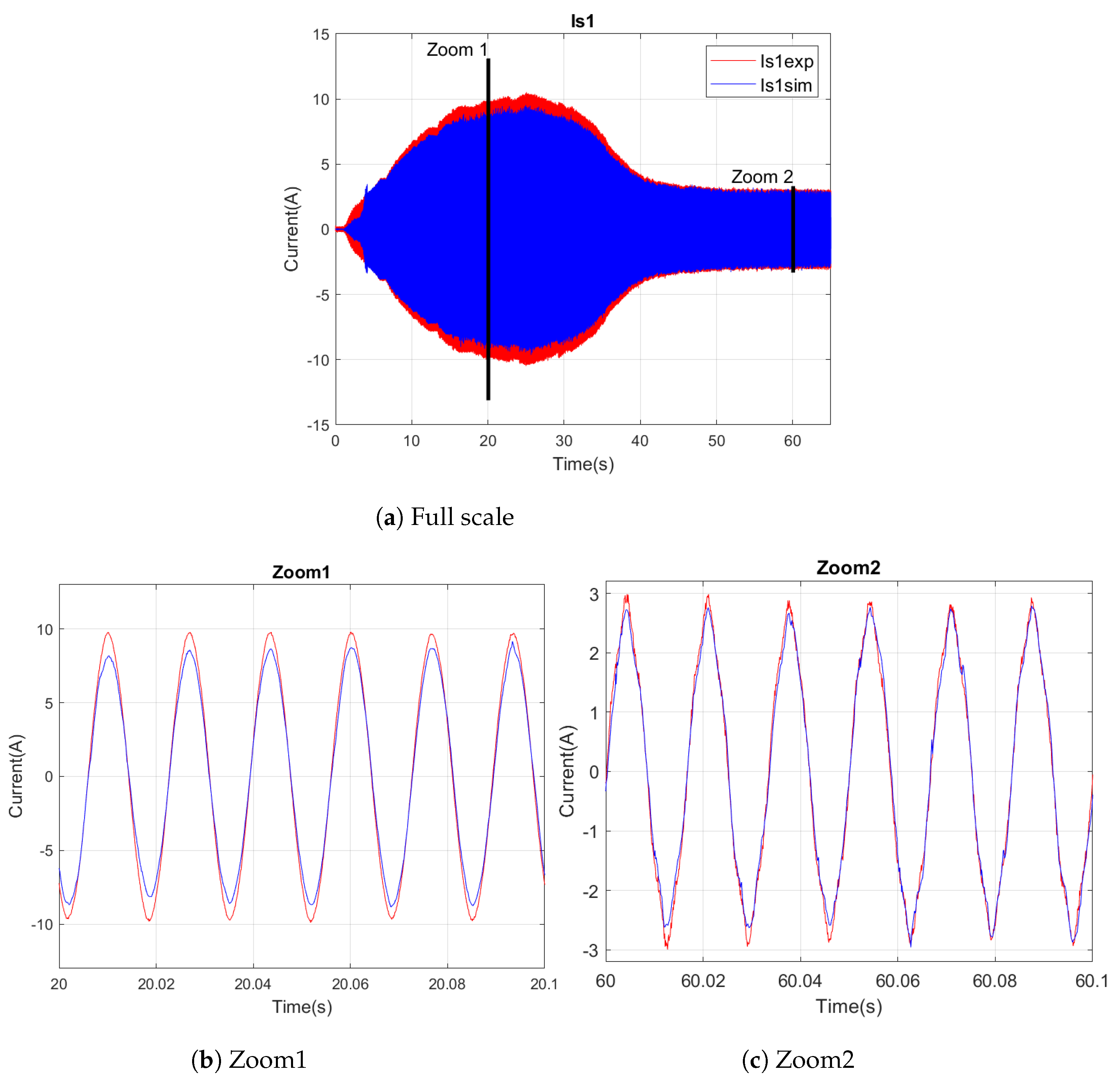
Figure 25 illustrates a comparison between the measured stator currents and the simulated ones during the start-up phase. The red curve represents the measured stator current, while the blue curve represents the simulation result. It is important to note that any differences observed before the first 4 s should be disregarded, as they are solely related to the operation of the speed and position estimator.
The largest difference appears in the amplitude of the current (Figure 25b), but the harmonic content of the current is generally very well reproduced (Figure 25c).
In Figure 25b, the amplitude error is about 18%, but it becomes less than 1% at the rated speed (Figure 25c).
Figure 26 shows a comparison of the rotor currents. The amplitude error reaches 5% in Figure 26b, but at nominal speed, the amplitude difference is about 1.2% (Figure 26d).
Here again, the currents are very well reproduced, and the effect of the spatial harmonics is very obvious.
An analysis of the results displayed in the graphs reveals an exceptional agreement between the measured experimental currents and those generated by the Simulink model. This near-perfect similarity was consistently observed throughout the experimental tests, providing robust evidence for the accuracy of both the model and the experimental parameter identification method employed.
The systematic superposition of these curves across various conditions and test parameters underscores the reliability of this digital twin. It demonstrates an impressive capability to accurately reproduce the actual behavior of the machine across diverse operational scenarios. Such fidelity is crucial for ensuring the reliability and effectiveness of the digital twin in practical applications.
6.2. Comparison of Several Copies of Identical Machines
To evaluate the sensitivity of this identification method, the simulated current waveforms of four examples of identical machines with the same geometry and characteristics were compared. The same simulation was repeated using the coupled-circuit model, replacing only the measured parameters of each machine.
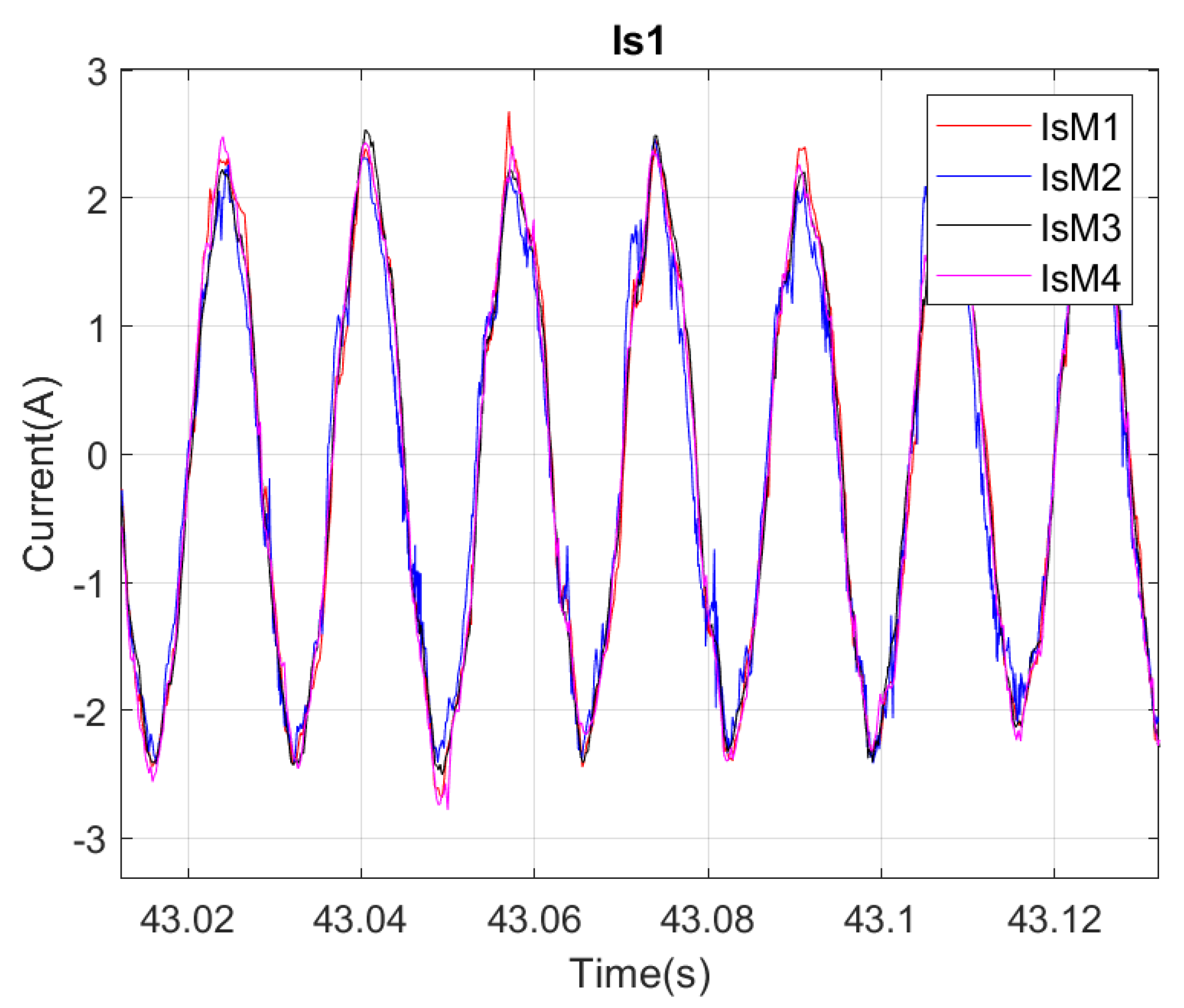
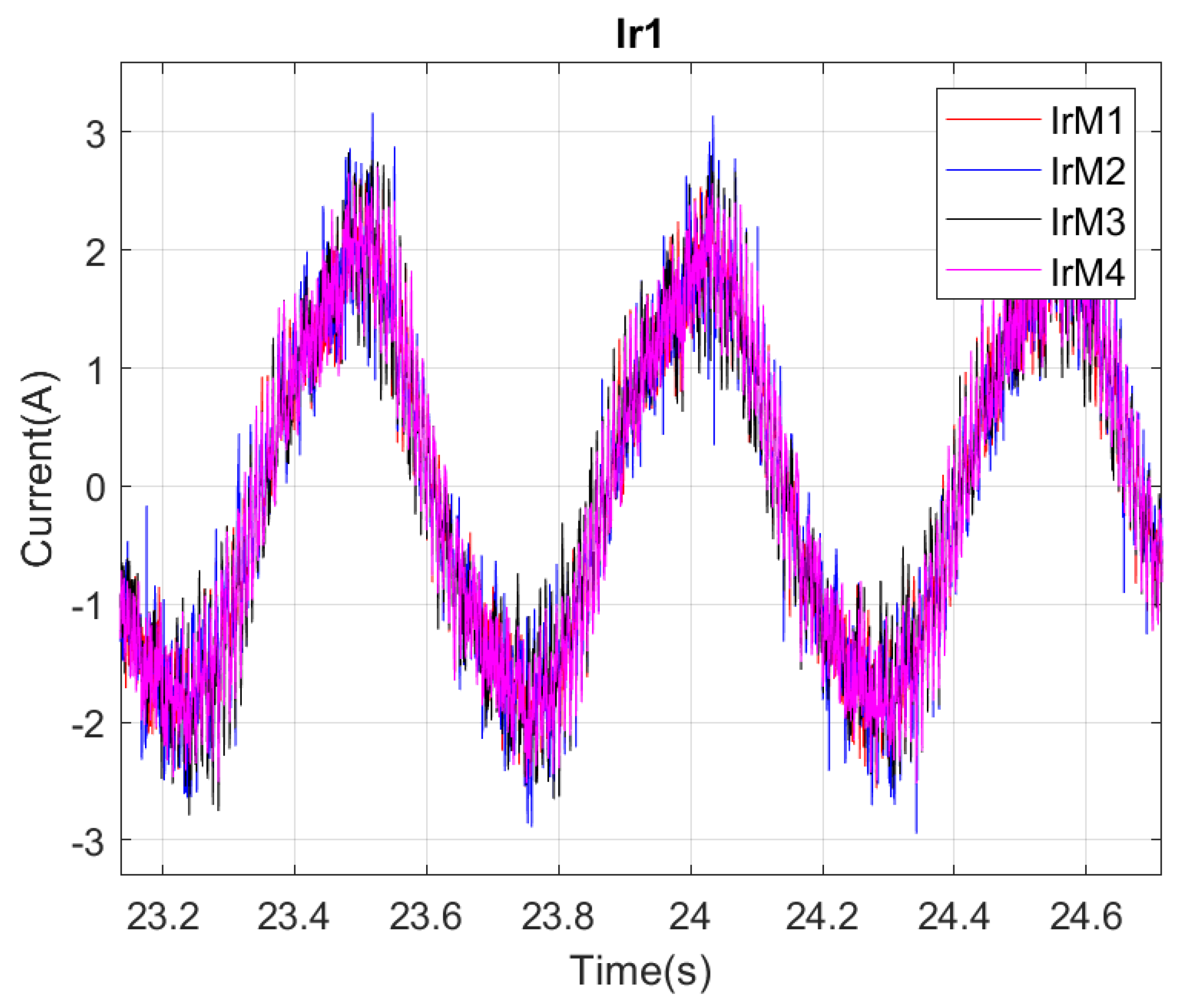
Figure 27 presents a comparison of the stator currents for operation at 1700 RPM, and Figure 28 shows the rotor current waveforms.
The signals are always very close, but the slight differences in parameters lead to specific oscillations, which are clearly observable in the currents. This shows that this model and the identification method developed are sufficiently sensitive to highlight the particularities of each machine. This is an essential characteristic for establishing a high-performance digital twin and for the development of diagnostic or aging analysis methods.
7. Conclusions
This study shows an innovative approach for the experimental identification of a coupled-circuit model, making it possible to develop a high-performance digital twin for a specific motor. This approach is based on simple, standstill electrical measurements and does not require specific data on the studied machine or expensive measuring equipment. Compared to identification methods based on the finite-element method, this experimental approach stands out for its speed and precision. The results align closely with those of a real machine. The identification of a machine is accomplished in half a day for 2880 discrete positions, and it is shown that there is a significant improvement in the results compared to the finite-element method. This allows for the creation of specific signatures for a given machine and the differentiation of supposedly identical machines from the same mass production.
Author Contributions
Conceptualization, F.Z.A. and J.C.; methodology, F.Z.A.; software, F.Z.A. and A.M.; validation, F.Z.A., A.M. and J.C.; formal analysis, F.Z.A., A.M. and J.C.; investigation, F.Z.A.; resources, F.Z.A.; data curation, F.Z.A.; writing—original draft preparation, F.Z.A.; writing—review and editing, F.Z.A. and J.C.; visualization, F.Z.A. and J.C.; supervision, J.C. and I.K.; project administration, J.C. and I.K.; funding acquisition, J.C. and I.K. All authors have read and agreed to the published version of the manuscript.
Funding
This work was supported in part by the Canada National Sciences and Engineering Research Council through Laval University, Grant ALLRP567550-21.
Data Availability Statement
Data sharing is not applicable to this article.
Conflicts of Interest
The authors declare no conflicts of interest.
Abbreviations
The following abbreviations are used in this manuscript:
| FEM | Finite-element method. |
| WRIM | Wound-rotor induction machine. |
| Machine #1. | |
| Relative error. | |
| Objective function error of finite-element method. | |
| Objective function error of Motor 1. |
Appendix A. The Dimensions of the Identified Asynchronous Machine
Table A1 presents the nameplate of our identified machine.

Table A1.
The nameplate of the wound-rotor induction motor (WRIM).
| Parameter | Value | Unit |
|---|---|---|
| Power | 2.5 | HP |
| Voltage | 208 | V |
| Number of Phases | 3 | |
| Frequency | 60 | Hz |
| Angular Velocity | 0.12 | rad/s |
| Number of Pole Pairs | 2 | |
| Power Factor | 0.81 | |
| Current | 8 | A |
| Temperature Rise | 40 | °C |
References
- Fernando, A.-G.; Antonio, G.; Sen, B.; Wang, J. Real-time hardware-in-the-loop simulation of permanent-magnet synchronous motor drives under stator faults. IEEE Trans. Ind. Electron. 2017, 64, 6960–6969. [Google Scholar]
- Ma, J.; Yuan, Y.; Chen, P. A fault prediction framework for Doubly-fed induction generator under time-varying operating conditions driven by digital twin. IET Electr. Power Appl. 2023, 17, 499–521. [Google Scholar] [CrossRef]
- Terron-Santiago, C.; Martinez-Roman, J.; Puche-Panadero, R.; Sapena-Bano, A. A review of techniques used for induction machine fault modelling. Sensors 2021, 21, 4855. [Google Scholar] [CrossRef] [PubMed]
- Sapena-Bañó, A.; Chinesta, F.; Pineda-Sanchez, M.; Aguado, J.; Borzacchiello, D.; Puche-Panadero, R. Induction machine model with finite element accuracy for condition monitoring running in real time using hardware in the loop system. Int. J. Electr. Power Energy Syst. 2019, 111, 315–324. [Google Scholar] [CrossRef]
- Pineda-Sanchez, M.; Puche-Panadero, R.; Martinez-Roman, J.; Sapena-Bano, A.; Riera-Guasp, M. Partial inductance model of induction machines for fault diagnosis. Sensors 2018, 18, 2340. [Google Scholar] [CrossRef] [PubMed]
- Yakhni, M.-F.; Cauet, S.; Sakout, A.; Assoum, H.; Etien, E.; Rambault, L.; El-Gohary, M. Variable speed induction motors’ fault detection based on transient motor current signatures analysis: A review. Mech. Syst. Signal Process. 2023, 184, 109737. [Google Scholar] [CrossRef]
- Ebrahimi, A. Challenges of developing a digital twin model of renewable energy generators. In Proceedings of the IEEE 28th International Symposium on Industrial Electronics (ISIE), Vancouver, BC, Canada, 12–14 June 2019; pp. 1059–1066. [Google Scholar]
- Bouzid, S.; Cros, J.; Viarouge, P. Real-time digital twin of a wound rotor induction machine based on finite element method. Energies 2020, 13, 5413. [Google Scholar] [CrossRef]
- Tessarolo, A. Accurate computation of multiphase synchronous machine inductances based on winding function theory. IEEE Trans. Energy Convers. 2012, 27, 895–904. [Google Scholar] [CrossRef]
- Wei, X.; Guangyong, S.; Guilin, W.; Zhengwei, W.; Paul, K.C. Equivalent circuit derivation and performance analysis of a single-sided linear induction motor based on the winding function theory. IEEE Trans. Veh. Technol. 2012, 61, 1515–1525. [Google Scholar]
- Houdouin, G.; Barakat, G.; Dakyo, B.; Destobbeleer, E. A winding function theory based global method for the simulation of faulty induction machines. In Proceedings of the IEEE International Electric Machines and Drives Conference, Madison, WI, USA, 1–4 June 2003; Volume 1, pp. 297–303. [Google Scholar]
- Gbégbé, A.Z.; Rouached, B.; Cros, J.; Bergeron, M.; Viarouge, P. Damper Currents Simulation of Large Hydro-Generator Using the Combination of FEM and Coupled Circuits Models. IEEE Trans. Energy Convers. 2017, 32, 1273–1283. [Google Scholar] [CrossRef]
- Elsherbiny, H.; Szamel, L.; Ahmed, M.; Elwany, M. High accuracy modeling of permanent magnet synchronous motors using finite element analysis. Mathematics 2022, 10, 3880. [Google Scholar] [CrossRef]
- Queval, L.; Ohsaki, H. Nonlinear abc-model for electrical machines using N-D lookup tables. IEEE Trans. Energy Convers. 2014, 30, 316–322. [Google Scholar] [CrossRef]
- Benninger, M.; Liebschner, M.; Kreischer, M. Automated Parameter Identification for Multiple Coupled Circuit Modeling of Induction Machines. In Proceedings of the International Conference on Electrical Machines (ICEM), Valencia, Spain, 5–8 September 2022; pp. 1307–1313. [Google Scholar]
- Rouached, B.; Bergeron, M.; Cros, J.; Viarouge, P. Transient fault responses of a synchronous generator with a coupled circuit model. IEEE Int. Electr. Mach. 2015, 32, 583–589. [Google Scholar]
- Mathault, J.; Bergeron, M.; Rakotovololona, S.; Cros, J.; Viarouge, P. Influence of discrete inductance curves on the simulation of a round rotor generator using coupled circuit method. Electrimacs 2014, 61, 19–22. [Google Scholar]
Figure 1.
Schematic representation of a three-phase wound-rotor asynchronous machine.

Figure 2.
Identification process.

Figure 3.
Wound-rotor induction machine [8].
Figure 3.
Wound-rotor induction machine [8].

Figure 17.
Sampling principle based on the rotor position.

Figure 18.
Procedure for calculating inductances with Matlab2021a.

Figure 19.
Shapes of identified inductances.

Figure 20.
Self-inductance, , with respect to the position.

Figure 21.
Mutual inductance, , with respect to the position.

Figure 22.
Self-inductance, , with respect to the position.

Figure 23.
Mutual inductance, , with respect to the position.

Figure 24.
Implementation of the coupled-circuit model in Matlab Simulink.

Figure 25.
Stator current during start-up test until steady-state operation.

Figure 26.
Rotor current during start-up test until steady-state operation.

Figure 27.
Stator current waveforms of the four identical motors.

Figure 28.
Rotor current waveforms of the four identical motors.

Table 1.
Comparison of least mean square errors for the initial position.
| FEM | |||||
|---|---|---|---|---|---|
| Test 1 | 62 | 50 | 61 | 51 | 53 |
| Test 2 | 50 | 52 | 48 | 39 | 45 |
| Test 3 | 79 | 45 | 49 | 38 | 52 |
| Test 4 | 143 | 50 | 47 | 43 | 53 |
| Test 5 | 66 | 52 | 51 | 44 | 54 |
| Test 6 | 100 | 57 | 71 | 44 | 54 |
| Test 7 | 64 | 73 | 152 | 21 | 46 |
| Test 8 | 57 | 71 | 51 | 38 | 53 |
| Test 9 | 78 | 41 | 62 | 45 | 44 |
| Test 10 | 166 | 53 | 64 | 31 | 47 |
| Test 11 | 51 | 40 | 44 | 12 | 41 |
| Test 12 | 63 | 20 | 59 | 49 | 25 |
| Test 13 | 104 | 49 | 49 | 41 | 53 |
| Sum of errors | 1081 | 651 | 805 | 494 | 618 |
| Comparison with FEM | 39% | 25% | 54% | 43% | |
| Comparison to | −24% | 24% | 6% |
Disclaimer/Publisher’s Note: The statements, opinions and data contained in all publications are solely those of the individual author(s) and contributor(s) and not of MDPI and/or the editor(s). MDPI and/or the editor(s) disclaim responsibility for any injury to people or property resulting from any ideas, methods, instructions or products referred to in the content. |
© 2024 by the authors. Licensee MDPI, Basel, Switzerland. This article is an open access article distributed under the terms and conditions of the Creative Commons Attribution (CC BY) license (https://creativecommons.org/licenses/by/4.0/).
Share and Cite
MDPI and ACS Style
Aboubi, F.Z.; Maïga, A.; Cros, J.; Kamwa, I. Experimental Identification of a Coupled-Circuit Model for the Digital Twin of a Wound-Rotor Induction Machine. Energies 2024, 17, 1948. https://doi.org/10.3390/en17081948
AMA Style
Aboubi FZ, Maïga A, Cros J, Kamwa I. Experimental Identification of a Coupled-Circuit Model for the Digital Twin of a Wound-Rotor Induction Machine. Energies. 2024; 17(8):1948. https://doi.org/10.3390/en17081948
Chicago/Turabian StyleAboubi, Fatma Zohra, Abdrahamane Maïga, Jérôme Cros, and Innocent Kamwa. 2024. "Experimental Identification of a Coupled-Circuit Model for the Digital Twin of a Wound-Rotor Induction Machine" Energies 17, no. 8: 1948. https://doi.org/10.3390/en17081948
Note that from the first issue of 2016, this journal uses article numbers instead of page numbers. See further details here.