
Influence of the TABS Material, Design, and Operating Factors on an Office Room’s Thermal Performance

AGH University of Krakow, Faculty of Mechanical Engineering and Robotics, Department of Power Systems and Environmental Protection Facilities, al. A. Mickiewicza 30, 30-059 Krakow, Poland
*
Author to whom correspondence should be addressed.
†
These authors contributed equally to this work.
Energies 2024, 17(8), 1951; https://doi.org/10.3390/en17081951
Submission received: 18 March 2024
/
Revised: 16 April 2024
/
Accepted: 17 April 2024
/
Published: 19 April 2024
(This article belongs to the Collection Energy Efficiency and Environmental Issues)
Abstract
:Reducing energy consumption in residential and commercial buildings is an important research topic. Thermally activated building systems are a promising technology for significantly reducing energy consumption. The high thermal inertia, large surfaces, and radiative nature are advantages of these systems, but, on the other hand, this makes the system control and design complex. A transient simulation is also required to address the dynamic behavior of the system. The influence of 19 factors (material, design, and operating parameters) on the air temperature and mean radiant temperature inside the room as well as the required cooling equipment power were analyzed to better understand the system. The screening experiment was conducted using the random balance design method, and measurement data were used to validate the resistance–capacitance model. The analysis was performed using the Plackett–Burman design and a design with randomly selected points from a full factorial experiment. The results show that internal heat gains and the inlet water temperature have a significant influence on the system, and the influence of the screed’s properties is insignificant compared to other parameters. It should be borne in mind that the obtained results and conclusions are valid for the assumed range of factors’ variability.
1. Introduction
Thermally activated building systems (TABS) are commonly used for heating and cooling multi-story buildings. They cover a wide range of various constructions [1], including one with pipes embedded in the concrete core of the slab. This type of TABS was introduced in Switzerland in the early 1990s and, since then, it has been installed in numerous buildings around the world [2]. TABS are known in German as Betonkerntemperierung (BKT) systems, or in English as Concrete Core Activation (CCA) or Concrete Core Cooling (CCC) [3,4,5]. During periods of high thermal load, heat is transferred through the floor and ceiling and stored in concrete; it can then be removed by water flowing in pipes when the occupants are absent [6]. Spreading the removal of heat over a longer period results in lower peak power requirements for cooling systems, which can lead to energy savings up to 50% [7].
The high thermal inertia, large surfaces, and radiative nature are advantages of TABS; however, on the other hand, this makes the system control and design complex. A transient simulation is also required to address the dynamic behavior of the system [8,9]. In [10], thermal comfort issues in a room located in an office building with TABS were experimentally investigated. Measurements performed during the everyday operation of the room revealed very low differences in indoor air temperature (between 22.5 °C and 23.1 °C during the working days) in its vertical profile and good thermal conditions provided by TABS cooperating with a balanced ventilation system. The average temperature of the floor’s surface ranged from 20.6 °C to 26.2 °C. However, this study was not oriented to dynamic thermal analysis of TABS. Such works are very rare because multi-floor buildings with thermally activated slabs exchanging heat between upper and bottom adjacent zones are, in general, large commercial facilities. Hence, they are normally very difficult to access, and measurements are very troublesome for occupants during their normal operation. That is why most of the experimental studies on TABS concern control-oriented applications in terms of energy use [11,12,13,14] or were performed under laboratory conditions in simple test rooms [15,16].
One way of estimating system performance is through computational fluid dynamics (CFD). It can provide detailed information about the system, but it is time-consuming and therefore impractical [17,18]. Simplified methods based on ordinary differential equations can be an alternative to detailed simulations because they require less time to solve. Nageler et al. [18] compared the results of CFD simulations and simplified physical models with measurement data. They found that simplified models can provide satisfying results. Sharifi et al. [9] used a simplified resistance–capacitance model of TABS to develop the control algorithm for optimal load splitting between TABS and the secondary cooling system. The utilization of the simplified model allowed authors to run the optimization algorithm for a one-year period (8760 h long time steps) within 2 h, which would not be possible with detailed simulations. To make the calculations easier, the method for simulating a room with TABS was standardized in ISO 11855-4 [19]. This standard proposes a one-dimensional simplified resistance–capacitance mathematical model of the room and slab, which is solved with the finite difference method (FDM). The method has been utilized by Behrendt [20] to develop a computer program for simulating TABS. Catalano [6] has modified the ISO 11855-4 method to deal with unrealistic behavior of the system in the case of high thermal load and low cooling power, which resulted in internal temperature exceeding 40 °C. The author has proposed a correction factor that was calculated based on air temperature inside the room and was used to modify heat gain value. However, simplified methods still require detailed information on room design as well as on internal and external conditions. Therefore, identifying parameters with the highest influence on the performance of TABS would simplify the calculations and result in a better understanding of the system.
Due to the complexity of TABS, many studies have been conducted to establish the influence of various parameters on conditions in the TABS-equipped building and control strategy. Lu et al. [21] examined building energy flexibility under the influence of various parameters that included thermal transmittance of the external wall (U-value), total structural thermal mass, internal heat gains, and methods of cooling. They found that the U-value of the external wall had a slight effect on cooling performance when compared to other parameters. It should be kept in mind that this is valid for the assumed input parameters’ variability range. Saelens et al. [22] evaluated the influence of occupants’ behavior on internal heat gains. They concluded that changes in various aspects of occupants’ behavior, such as their mobility, the probability that they appear in the office during the day, or manual operation of the lights and shading devices, have a significant influence on cooling demand and thermal comfort in the office. Their results show that switching off the lights reduces cooling demand by 8% and shortens the time that the temperature is outside the thermal comfort zone by 15%. Rijksen et al. [23] examined the influence of internal heat gains and window area on the peak-shaving performance of cooling in an office building with TABS and without it. The authors discovered that TABS combined with a smaller area of the windows resulted in a reduction of required cooling power by 50% when compared to a system without energy buffering. Samuel et al. [24] experimentally assessed the effect of parameters on thermal comfort in a room with TABS installed. The authors concluded that increasing the number of cooling surfaces had a positive effect on thermal comfort and that, with all surfaces cooled (ceiling, floor, and four walls), thermal comfort was maintained throughout the day. They also found out that the use of ventilation could result in rapid temperature changes as external air was mixed with internal. Ning et al. [25] examined the influence of geometric and thermal parameters on the system response time. They found that concrete thickness and pipe spacing have a significant impact on TABS response time. Samuel et al. [26] performed a sensitivity analysis based on CFD simulations to investigate the influence of pipe diameter, pipe thermal conductivity, and slab thickness on thermal comfort in a room with TABS. They found that increasing pipe thermal conductivity from 0.14 to 1.4 and increasing its inner diameter from 9 to 17 mm reduced the operative temperature by 2.8 °C and 1.8 °C, respectively. However, increasing the floor and ceiling slab thickness from 0.1 to 0.2 m reduced the operative temperature by only 0.3 °C. Chandrashekar and Kumar [27] experimentally studied the influence of various floor covering materials on TABS performance. They found that using a granite floor resulted in lowering air temperature in the room by 1.5 °C and reduced cooling load by 10% compared to the vinyl floor, which had lower thermal conductivity than granite. Rakesh et al. [28] experimentally evaluated the influence of inlet water velocity on the temperature in a room with TABS. They found that increasing the water velocity from 0.35 to 1 reduced internal air temperature by 1.5 °C; however, further a increase in the water velocity to 1.5 reduced air temperature by only 0.2 °C. The review presented in this section has been summarized in Table 1.
As presented above, materials, design, and operating parameters have important effects on the performance of TABS. However, the influence of these parameters has not been widely discussed in terms of the internal air and mean radiant temperature, which is very important in terms of thermal comfort. Moreover, the researchers examined the influence of a limited number of factors at the same time (all factors at a time analysis). Therefore, the possibility of comparing the influence of the parameters is limited. To fill those gaps, we conducted a sensitivity analysis based on a random balance design and found which parameters significantly affect the temperature inside a room with TABS and required cooling power. We examined the influence of 19 parameters, including the slab material properties, properties of walls, circuit operating parameters, and heat gains. The calculations were performed using the modified method presented in ISO 11855-4 [19] and validated using measurement data.
2. Details of Research Objective
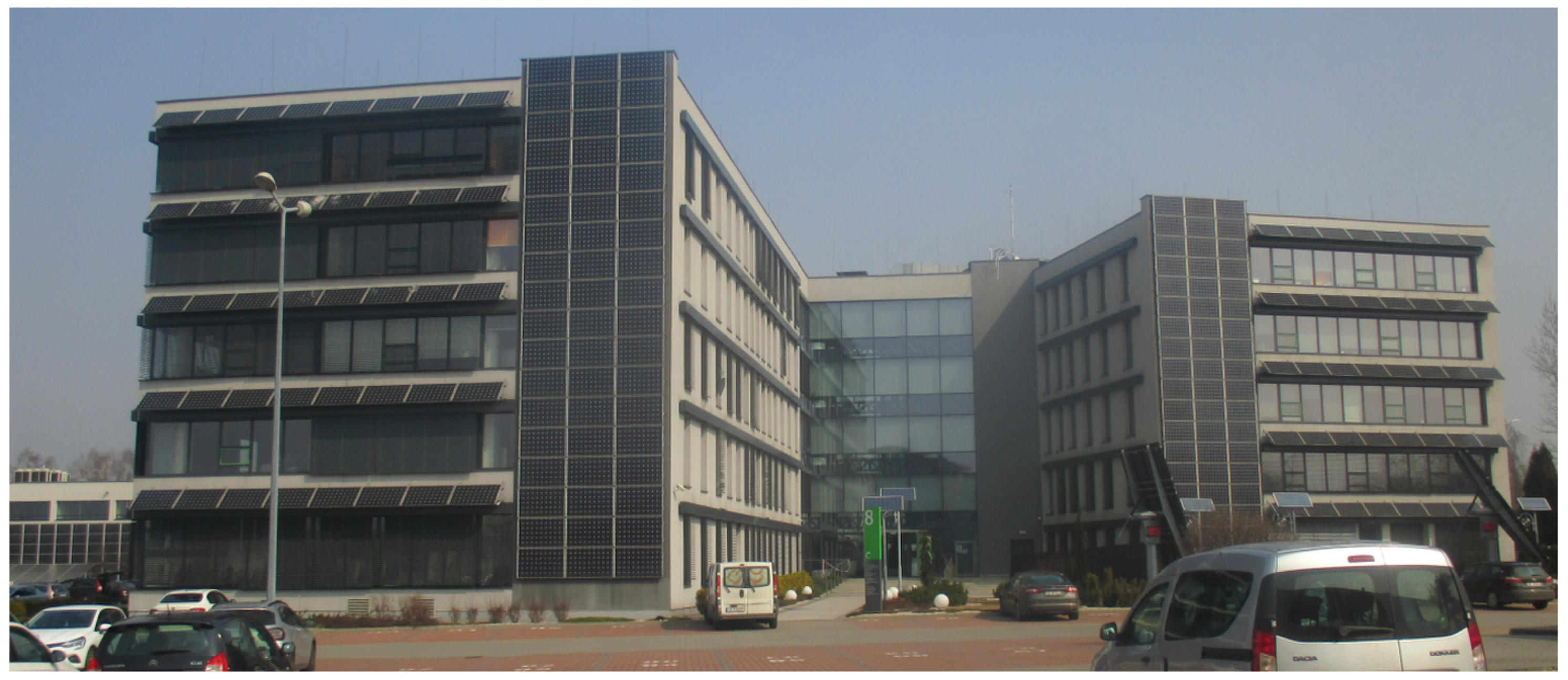
The experimental part of this study was performed in a single office room in the passive office building (Figure 1) located in Katowice in south Poland. This facility has been described recently [10,29]. It has a total and usable area of 8100 m2 and 7500 m2, respectively.
Ceiling slabs (Figure 2b) and the basement floor were made from 30 cm thick reinforced concrete with embedded modules and with polymer pipes with a total area of 4500 m2 and 1870 m2, respectively. This is the main heating and cooling system in the building. It is supported by five air handling units with heating and cooling coils, creating a complete heating, ventilation, and air conditioning (HVAC) system. Four units have a common intake and exhaust collector on the roof, and they supply fresh air to office and social rooms. The fifth unit supplies fresh air to sanitary facilities and toilets and is equipped with a separate air intake and exhaust on the roof. The HVAC system is supplied with water from the set of six water/water heat pumps with a total heating and cooling capacity of 244 kW and 187 kW, respectively. Additionally, 10 vacuum solar collectors are used to support the heating and tap water systems. As a peak cooling source, two chillers can be used.
The office rooms are located around the outer perimeter of the building, facilitating the use of daylight. The large area of triple-glazed external windows (U = 0.7 ) increases the share of solar energy in the thermal balance of the building. External blinds, on the other hand, make it possible to reduce excessive solar gains during the summer. The corridors are located on the inner perimeter of the building and, thanks to the glazing in its central part, they are naturally illuminated. Photovoltaic modules with a total power of 107 kWp mounted on the roof and on the facade, as well as the three trackers in front of the building, reduce electricity consumption in the building. For effective energy management and data analysis, a building management system (BMS) is used. An office room (Figure 2a), located on the west side of the second floor of the building was chosen for the research. It has a floor area of 46.11 m2 and a height of 3.10 m. During measurements, it was not occupied.
3. Research Strategy
A sensitivity analysis for 19 (material, design, and operating) parameters for the real TABS is impossible due to the high cost and the long time needed to perform each experiment. One solution is to perform a series of simulation experiments. There are basic CFD-based calculations that are detailed and accurate but time-consuming, so reduced-order methods for the calculation of such complex systems are required. However, even the use of supercomputers and distributed computing to perform sensitivity studies for 19 parameters is time-consuming. Therefore, there is a need to utilize an efficient research strategy by using effective and time-reducing methods.
3.1. Research Algorithm
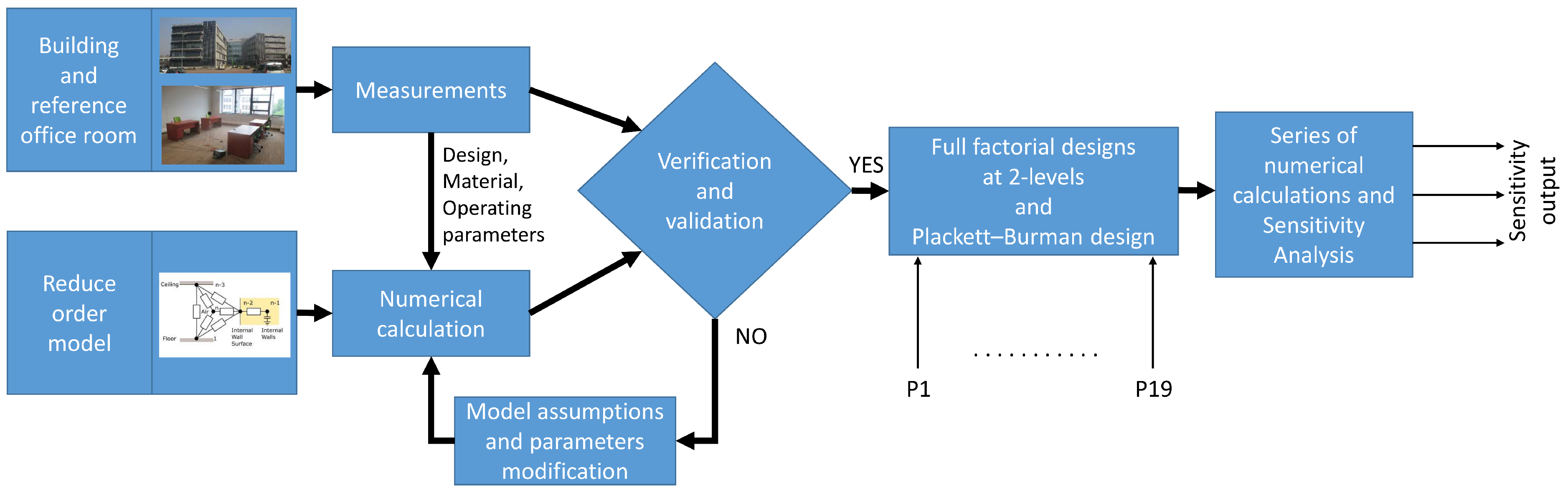
According to the research algorithm outlined in Figure 3, the initial phase of the study involved meticulous identification of design specifications, material properties, and operational parameters of the building room with TABS (Section 2). Simultaneously, a decision was made to adopt a reduced computational model, aligning with the established methodology outlined in ISO 11855-4 [19] (Section 5). The assumed computational model of the office room with TABS was verified and validated (Section 5.2) using measurement results (Section 4). The mean air temperature and mean radiant temperatures of the room were compared in the validation analysis. For a full factorial design experiment, there was a need to conduct = 524,288 computational experiments. It is still impossible to conduct the full experiment due to time-consuming calculations.
It was decided to conduct research using the random balance design method, and experiments were generated by the use of the Plackett–Burman (PB) design. The PB designs are mainly used for screening research. This design is efficient, but the main effects are, in general, heavily confounded with two-factor interactions. For this reason, we decided to extend this research and conduct 512 randomly selected experiments from a full factorial design. This allowed the results to be confirmed or rejected. Consequently, we assess the impact of 19 factors on five output parameters. This screening experiment has been performed using scripts written in Python 3.10, and the pyDOE3 version 1.0.1 [30] library has been used to prepare the design of the experiments.
3.2. Assumptions
Using data from diverse sources, an extensive array of cases within the TABS across varied geographical locations can be analyzed. The ranges of variability (Table 2) in the parameters under analysis were determined by synthesizing information based on existing literature. Consequently, we assumed parameters such as a cooling surface area () equal to 50% and 100% of the total floor area on low and high levels, respectively, and the material parameters’ variability values. The thermal conductivity of the concrete layer () and pipe spacing () are limited by the assumptions of the method described in [19]; the thermal conductivity, the specific heat, the density of the screed layer (, , ), the specific heat, and the density of the concrete layer (, ) are based on [31].
The construction of the slab is based on Figure 2b, and properties of the 2nd layer (screed) and the 3rd layer (concrete) have been considered as parameters in the sensitivity analysis. The water pipes were always located in the middle of the concrete layer. The 1st layer (carpet) has been ignored due to its negligible thermal capacity; hence, it has not been considered a slab layer in the numerical model (there is no node representing the carpet layer). However, the influence of the thermal resistance of the carpet has been examined by introducing additional thermal resistance () at the floor. We have assumed that, at the high level, the value of is equal to the thermal resistance of the carpet in the considered room, and the low level of the parameter represents the situation where the carpet is not present and therefore the additional thermal resistance is equal to 0 . The properties of the 4th layer (plaster gypsum) have been considered constant in the sensitivity analysis, and they are presented in Table 3.
The internal building walls consist of two layers of plasterboard and a layer of mineral wool between them. Their structure is the same as in the building for which the measurements were made. The high level for the internal wall thickness parameter decomposed into layers equaled 25 mm for plasterboard and 200 mm for the mineral wool layer () and, for the low value, . To calculate internal walls’ thermal resistance and specific heat capacity, which are the parameters in the mathematical model, we have evaluated the substitute values of walls’ thermal conductivity () and specific thermal capacity () according to the following equations:
where is thickness of the ith layer [m], is the thermal conductivity of the ith layer [], is the specific heat of the ith layer [], and is the density of the ith layer []. The thermal properties of the walls’ materials were determined according to [31]. The values of and are presented in Table 3.
The values of water flow () and inlet water temperature () have been estimated according to measurement results. The values of the parameters at low and high levels denote the minimum and maximum values provided by the building management system (BMG), respectively.
Thermal transmittance of window variability is based on values provided by [32]. We have assumed that the values of the window area () equaled 30% and 70% of the external wall area at the low and high levels, respectively. Additionally, we have assumed that the area of glazing () used in the process of calculating solar heat gains equals 90% of the total window area ().
Thermal transmittance of the opaque part of the external wall () is calculated according to [33]. The wall consists of four layers: (i) plaster, (ii) styrofoam with a thickness of 300 mm, (iii) hollow bricks, and (iv) plaster. The values of the parameter were determined by changing the thickness of the styrofoam layer, and for low and high values, the thickness was equal to 50 mm and 300 mm, respectively.
The values of primary air gains () have been based on the results of measurements conducted in the considered room. The ventilation system provided constant airflow of 95 between 3 a.m. and 7 p.m.; however, the difference between supply and exhaust air temperature was greatest between 3 a.m. and 9 a.m. After 9 a.m., the difference between the supply and exhaust air temperature was reduced significantly; hence, the heat gain was considered to be 0 W despite the ventilation system still working. To simplify the model, we have assumed that the ventilation system provides constant airflow of 240 , which is the maximum value that can be provided by the HVAC system. To estimate the value of the parameters, we have assumed that the difference between supply and exhaust air temperature equals −4.5 °C and 0 °C at low and high levels, respectively, which results in the value of equal to −350 W and 0 W, respectively.
Internal heat gains () originate from occupants, office equipment, and lighting in the room. In a sensitivity analysis, we have assumed that the occupants are present and that they use the equipment between 7 a.m. and 5 p.m.; otherwise, the internal heat gains are equal to 0 W. We have determined that the value of the parameter at a low level, assuming that the room is not used, is 0 W. For the high level, the value of internal heat gains was estimated according to [34]. To carry out the calculations, we have assumed that five people work in the room and that each person uses a personal computer with two monitors; additionally, there is one printer in the room. The internal heat gains estimated according to those assumptions are equal to 1500 W. We have assumed that half of the internal heat gain is transferred through radiation () and the other half is through convection () [22]. All parameters considered in the sensitivity analysis along with their variability ranges are presented in Table 2.

Table 2.
Variability ranges of the input parameters.
| No | Parameter | Symbol | Value | Unit | |
|---|---|---|---|---|---|
| Low | High | ||||
| P1 | Cooling surface area | 23 | 46 | m2 | |
| P2 | Concrete thermal conductivity | 1.15 | 2 | W/(m·K) | |
| P3 | Screed thermal conductivity | 1.4 | 1.8 | W/(m·K) | |
| P4 | Concrete-specific heat | 900 | 1100 | J/(kg·K) | |
| P5 | Screed-specific heat | 900 | 1100 | J/(kg·K) | |
| P6 | Concrete density | 1800 | 2400 | kg/m3 | |
| P7 | Screed density | 1800 | 2000 | kg/m3 | |
| P8 | Concrete layer thickness | 0.2 | 0.4 | m | |
| P9 | Screed layer thickness | 0.005 | 0.03 | m | |
| P10 | Internal wall thickness | 0.066 | 0.25 | m | |
| P11 | Floor additional resistance | 0 | 0.032 | m2·K/W | |
| P12 | Water flow | 0.028 | 0.08 | kg/s | |
| P13 | Pipe spacing | L | 0.15 | 0.3 | m |
| P14 | Window area | 5.4 | 12.5 | m2 | |
| P15 | Thermal transmittance of window | 0.5 | 3.3 | W/(m2·K) | |
| P16 | Thermal transmittance of external wall (opaque) | 0.088 | 0.203 | W/(m2·K) | |
| P17 | Primary air heat gain | 1 | 0 | W | |
| P18 | Internal heat gains | 0 | 1500 2 | W | |
| P19 | Inlet water temperature | 16 | 22 | °C | |
1 Between 3 a.m. and 9 a.m.; otherwise 0 W. 2 Between 7 a.m. and 5 p.m.; otherwise 0 W.
To provide information about thermal comfort inside the room and the cooling power necessary for maintaining constant water temperature in the circuit, we have selected the following output parameters:
- Maximum and minimum air temperature (, ),
- Maximum and minimum mean radiant temperature (, ),
- Maximum power received by the circuit ().
The maximum/minimum air temperature (, ) and maximum/minimum mean radiant temperature (, ) have been considered only between 7 a.m. and 5 p.m. when occupants are present, while power () received by the circuit has been considered throughout the day.
Other parameters that have not been considered in the sensitivity analysis but that are necessary for calculations are presented in Table 3.
Table 3.
Other system parameters.
| Parameter | Symbol | Value | Unit |
|---|---|---|---|
| Room width | X | 5.8 | m |
| Room length | Y | 7.95 | m |
| Room height | Z | 3.1 | m |
| Convection coefficient on the floor | W/(m2·K) | ||
| Convection coefficient on the ceiling | W/(m2·K) | ||
| Convection coefficient on the internal walls | W/(m2·K) | ||
| Radiant heat transfer coeff. between floor and ceiling | W/(m2·K) | ||
| Radiant heat transfer coeff. between floor and internal walls | W/(m2·K) | ||
| Ceiling additional resistance | 0 | m2·K/W | |
| Water-specific heat | 4183 | J/(kg·K) | |
| Plaster layer thickness | m | ||
| Plaster thermal conductivity | W/(m·K) | ||
| Plaster-specific heat | 1000 | J/(kg·K) | |
| Plaster density | 1200 | kg/m3 | |
| Internal wall thermal conductivity | W/(m·K) | ||
| Substitute internal wall-specific thermal capacity | J/(m3·K) | ||
| Pipe external diameter | m | ||
| Pipe wall thickness | s | m | |
| Pipe wall thermal conductivity | W/(m·K) | ||
| Time step | 3600 | s | |
| Maximum iteration error allowed | °C | ||
| Maximum number of iterations allowed | - |
4. Details of Measurements
The measurements were carried out in a specially prepared office room with 46.11 m2 (Figure 2a). All sensors were placed in the room according to the layout presented in Figure 4a,b. For the sake of clarity, supply and exhaust channels of the ventilation system were indicated only for the ceiling.
All air and surface temperature measurements were performed using Pt100 platinum resistance sensors. Heat flux of the ceiling and the floor was measured using the HFP01 sensors of Hukseflux [35]. Global solar irradiance entering the room was measured by the LP PYRA03 pyranometer of DeltaOhm [36]. At the center of the room, a tripod was placed with a globe temperature sensor (diameter of 150 mm) at a height of 1.5 m. Based on [37,38], it was assumed that the mean radiant temperature is the same as the measured globe temperature. However, as noted in [39,40], this assumption may result in underestimation of the mean radiant temperature. As the room was unoccupied during measurements, this effect was minimized, but its precise assessment requires further analysis. Additionally, three air temperature sensors were attached to a tripod at heights of 0.2 m, 0.6 m, and 1 m above floor level. They were covered with low-emissivity () coating to minimize the impact of heat transfer by radiation. The wall temperature sensors were placed 1.5 m above the floor. All sensors are listed in Table 4. All sensors were connected directly to the Fluke 2638A data logger [41].
According to [43], combined uncertainty of measured variable x, when using a measurement sensor and a signal processing and display unit (device), is given by:
Both sensor and device uncertainties can be obtained from the relevant standards or manufacturer documentation. Following IEC 60751 [42] for the known temperature (T), the tolerances of the A and AA class sensors are given by the following relationships, respectively:
At 25 °C for the A class sensor, we obtain from Equation (4): = 0.116 °C. According to the manufacturer [41], for a 4-wire Pt100 sensor, uncertainty = 0.024 °C at 25 °C. Hence, from Equation (3): °C. Apart from variables listed in Table 4, inlet water temperature and flow rate were obtained from the heat meter connected to the BMS. For the second class heat meter [44] the maximum permissible error (MPE), expressed in %, is defined for the flow rate () and for the temperature difference measured by the pair of sensors () by the following relationships:
where means flow rate, is the maximum permissible flow rate, is the current inlet/outlet temperature difference, and is the minimum temperature difference ( = 5 K in the considered case). Based on available data, it was established that both and do not exceed 3%. Finally, according to the manufacturer’s data, it was assumed that the ventilation flow rate was measured with an accuracy of ±5%. The most troublesome to assess is the accuracy of heat flux sensors. Following the manufacturer’s recommendations [35] in buildings physics, it varies from ±6% in ideal conditions to ±20% in typical on-site applications. In the presented case, the second value seems to be reasonable in the analysis of the measurement results.
5. Computational Model Description
5.1. Mathematical Model Description
The mathematical model of the room is based on resistance–capacitance simplification introduced in ISO 11855-4 [19]. The mathematical model includes the slab, internal walls (walls between the considered room and adjacent ones), and air filling the room, which are divided into thermal nodes and, in each node, the heat balance is calculated according to the following equation:
where C is the thermal capacity of the node [], and the right-hand side of the equation is the sum of heat transfer rates received or delivered to the considered node in [W].
The RC representations of the slab and the room are presented in Figure 5a and Figure 5b, respectively. The heat transport in the slab is simplified by the use of the thermal resistance method provided in ISO 11855-2 [45], where is the thermal resistance between inlet water and concrete at the pipe level. It is introduced to calculate heat transfer between water flowing in pipes and concrete. In the part of the mathematical model representing the room, nodes representing the floor, ceiling, and internal wall surface are connected, which represents radiant heat transfer between them. The convective heat transfer is also present, and it is represented by connections between surface nodes and air nodes. Several simplifying assumptions were also made:
- The heat transport in the perpendicular direction to the floor is taken into consideration,
- Water mass flow in the pipes is constant throughout the simulation time,
- Radiant heat gains are distributed evenly to all surfaces,
- Conditions in rooms above and below are the same as in the considered room,
- All thermophysical properties are constant and independent of temperature.
The mathematical model is solved through the implicit scheme of the finite difference method, and the equation used for calculating temperature in the considered node can be written as follows:
where is the temperature of the considered node in the previous time step [°C], is the temperature of the previous node [°C], is the temperature of the next node [°C], is total radiant heat gain [W], is total convective heat gain [W], and is inlet water temperature [°C]. H represents the heat transfer coefficients, which depend on the type of node that is currently being considered. An iterative method is used for determining temperatures in the nodes, and with each iteration, the error is calculated as follows:
where is the temperature calculated in the previous iteration. Calculations are carried out until the iteration error is smaller than the maximum allowed error () or until the maximum number of iterations () is achieved. The values of maximum iteration error and maximum iterations allowed are presented in Table 3.
The initial and specific conditions have to be determined before calculating the heat delivered or received from the considered room. Specific conditions can be divided into three categories:
- Radiant heat gains delivered to surface nodes (floor, ceiling, and internal wall surface (Figure 5b)),
- Convective heat gains delivered to the air node,
- Heat received by the circuit from the pipe-level node.
Both radiant and convective heat gains depend on internal and external conditions and are calculated for every time step of the simulation according to the following equations:
where is the transmission heat gain [W], is the solar heat gain [W], is the primary air heat gain [W], and and are internal radiant and convective heat gains [W], respectively. The value of each term in Equations (11) and (12) has to be known for every time step of the simulation. Primary air and internal heat gains have been determined according to measurement data and the literature (see Section 3.2). The solar heat gains have been determined according to the following:
where is total solar irradiance entering the room [], and is the area of glazing [m2].
According to Catalano [6], adopting the value of transmission heat gain independent of temperature may lead to errors. Hence, the value of the transmission heat gain has been determined using the difference between external and internal temperatures according to PN-EN 12831-1 [46], and it is equal to the following:
where is the thermal transmittance of the opaque part of the external wall [], is the thermal transmittance of the window [], is the area of the opaque surface [m2], is the area of the window [m2], and is the external temperature [°C]. Since transmission heat gain is dependent on air temperature, it has to be calculated with every iteration. The external temperature has been obtained from weather data. To examine the influence of external conditions on the room, the weather data chosen for the experiment contained outside temperatures differing from measured room temperatures. The maximum value of the external temperature considered in the experiment was equal to 18 °C.
Convective heat transfer coefficients on the surfaces in the room were calculated according to equations developed by Awbi [47], presented in Table 5. It is assumed that the difference between the surface and air temperatures () in each case is constant and equal to 1.5 K, so the coefficients are constant.
The initial temperature of the nodes has been set to 22 °C by default. However, due to the high thermal inertia of the system, the time required by the node temperatures to reach their final distribution may exceed the simulation time. For that reason, a startup period has been added to the simulation [20]. During the startup period, node temperatures can reach their final values without altering the solution. To verify whether the final results are achieved, the difference between the maximum temperatures of the considered and the previous day is calculated. If the difference is smaller than 0.005 K, the solution is considered valid.
5.2. Validation and Verification
The mathematical model was validated using experimental data to assess whether the model parameters and the specific conditions are properly set. During the process, a six-day-long period was simulated, and the results were compared with data collected during measurements. The specific conditions were based on measurements of solar irradiation, external temperature, and air temperature delivered by an air conditioning system. Since there were no occupants in the room during the measurements, the internal heat gains resulted from measurement equipment only. They were assumed to have a constant value of 10 W throughout the simulation time. The specific conditions used in the simulation have been doubled to form a startup period; therefore, the total simulation time was equal to 12 days, but only the second half of it was considered valid and not affected by initial conditions. The simulation was performed with a time step () equal to 1 h and a maximum iteration error () equal to K.
A comparison of simulation results and measurements for air temperatures is presented in Figure 6a. The mean absolute error is equal to 0.16 °C, and the maximum error is 0.65 °C, which are acceptable values. In the case of mean radiant temperature, the error values were higher when compared to the air temperature mean, and the maximum absolute errors are equal to 0.18 °C and 2.02 °C, respectively. The high value of the maximum error may result from high sun radiation entering the room and heating the thermometer responsible for collecting the data. Despite the relatively high maximum error for the mean radiant temperatures, both air and radiant temperatures show good agreement with experimental data.
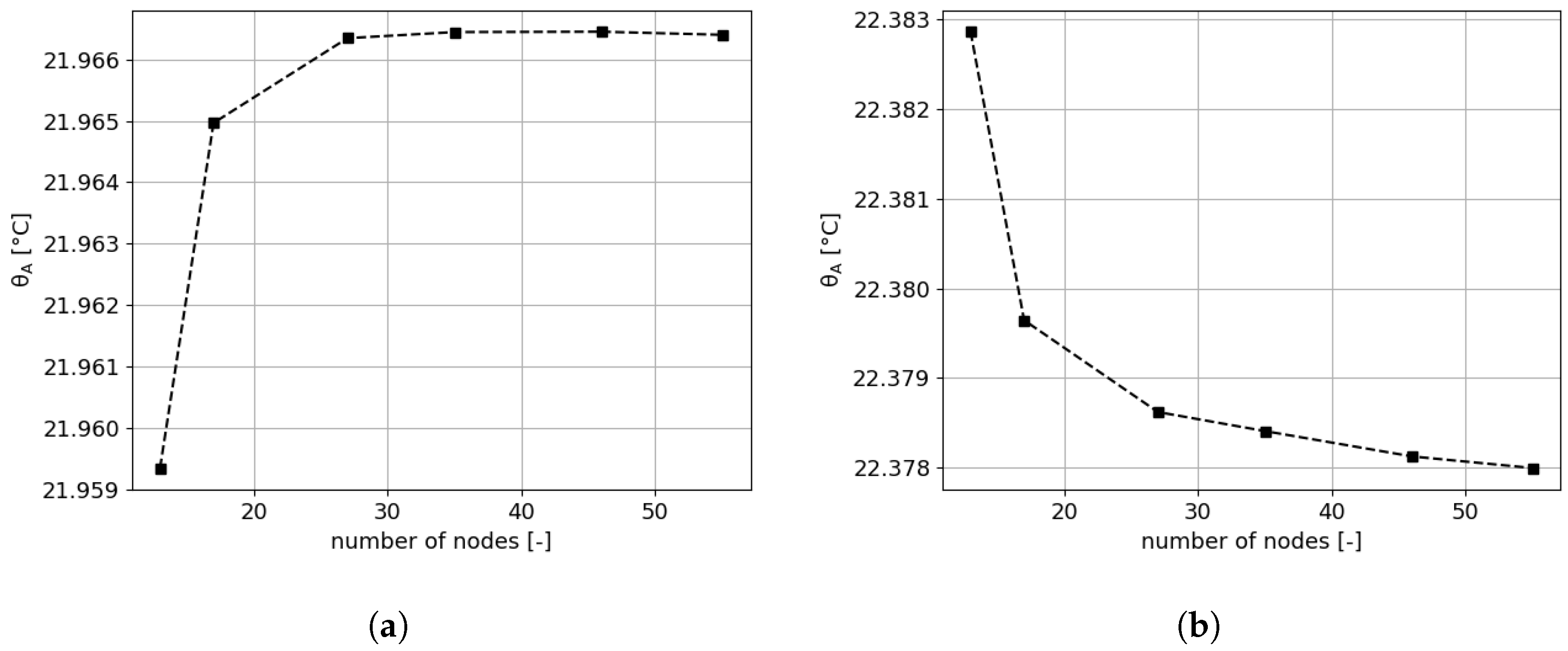
To assess that the results would converge, a grid independence study was conducted. A calculation with the number of nodes varying from 13 to 55 was considered. The grid independence study was performed for the air temperature at 12 a.m. and at 11 a.m. on the first day of the simulation time (1st and 12th time steps, respectively, after rejecting the startup period). The results are shown in Figure 7a and Figure 7b, respectively. In both cases, temperatures reach a steady value, with the number of nodes equal to 35. Beyond this value, no significant change in the solution can be reported; thus, we have chosen the model with approximately 35 nodes for sensitivity analysis. However, the number of nodes may differ depending on the experiment, since the geometry of the slab varies, as the thickness of the screed and concrete layer are parameters in the sensitivity analysis.
6. Results of Sensitivity Analysis
The sensitivity analysis was conducted using two experimental design methods—Plackett–Burman and full factorial design—from which 512 experiments were randomly selected. The medians of the appropriate output parameters were calculated for a series of design points when the specific factor assumed low or high levels. Scatter diagrams with marked medians (dashed lines) for all design points and medians for low and high levels (point) for both methods are presented in Figure 8, Figure 9, Figure 10, Figure 11 and Figure 12. The influence of the parameters’ changes on maximum air temperature () is presented in Figure 8. According to both experiment designs, the area of the cooling surface (), internal heat gains (), and inlet water temperature () have a significant impact on , as the differences in their medians have values greater than 2.2 °C. In the case of water flow (), the difference in the medians obtained with the full factorial design is at the same level as the difference in the area of the cooling surface (). However, the value obtained with the PB design is lower and equals 0.6 °C. Since the full factorial design contains more experiments, it is considered to be more informative in the case of uncertainty; therefore, parameter is also considered to have an impact on . The influence of the specific heat of concrete () cannot be confirmed, since its influence should be considered according to PB design. In contrast, according to full factorial design, its influence is negligible. The discrepancy between the two methods suggests that further study may be necessary to evaluate the impact of the concrete-specific heat.
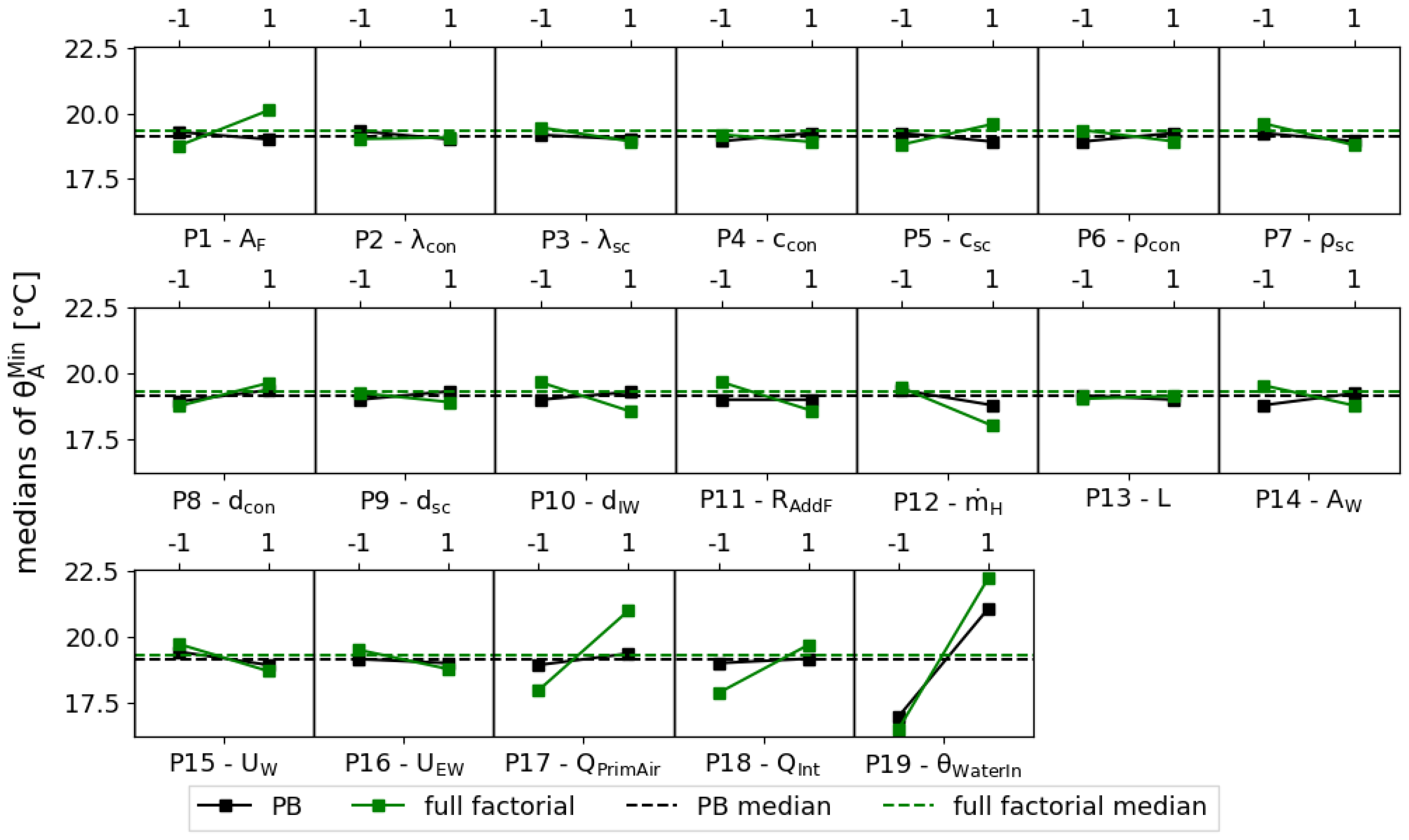
In the case of minimum air temperature () presented in Figure 9, the assumed DOEs show more inconsistency compared to the case of . According to the PB design (dark lines), only the inlet water temperature () has a significant impact on , with the difference in the medians equal to 4.1 °C, while for other parameters, the difference in the medians is smaller than 1 °C. However, according to the full factorial design, the area of the cooling surface (), internal wall thickness (), floor additional resistance (), water flow (), thermal transmittance of the window (), primary air heat gains (), internal heat gains (), and inlet water temperature () have considerable influence on , with the difference in the medians above 1 °C. Due to the more informative nature of the full factorial design, we consider parameters , , , , , , , as influences on .
The result of sensitivity analysis for the maximum value of mean radiant temperature () is presented in Figure 10. Both methods indicate that the cooling surface area (), internal heat gains (), and inlet water temperature () have a significant influence on the results, with differences in the medians greater than 1 °C. The results of the PB design indicate that the specific heat of concrete (), screed density (), and the window area () also have considerable influence on the maximum value of the mean radiant temperature. However, this is not confirmed by the results of the full factorial design, according to which the differences in the medians for parameters , , and are smaller than 1 °C. Therefore, the influence of parameters and is not considered significant. The significance of the window area () cannot be confirmed. According to the PB design, the difference in the medians is equal to 2.3 °C; however, the value obtained with a randomly selected design from a full factorial experiment equals 0.7 °C. Due to the inconsistency between the results of both methods, further study is necessary to confirm the influence of parameter .
The results for minimum mean radiant temperature () are presented in Figure 11. Similarly to the case of minimum air temperature (), the results obtained with the PB design indicate that only the influence of the inlet water temperature () can be considered significant, with the difference in the medians equal to 5 °C. The significance of parameter is confirmed by the results of the full factorial design, with the difference in the medians equal to 5.7 °C. The results obtained with the full factorial design indicate that the parameters , , , , , , and should also be considered significant. However, further study may be necessary to establish the influence of these parameters. According to both methods, the differences in the medians for thermal conductivity of concrete (), concrete-specific heat (), and distance between pipes () are smaller than 0.6 °C, which means that the influence of these parameters on is negligible.
The last output parameter examined in this study was the maximum power received by the circuit (). Its value corresponds with the power required by water cooling equipment to maintain the constant inlet water temperature. According to the results presented in Figure 12, both DOEs indicate that the cooling surface area (), thermal transmittance of the window (), and internal heat gains () have a significant impact on the value of , with the differences in the medians greater than 120 W. The results of both methods show that the properties of the screed layer (parameters , , and ) and thermal transmittance of the opaque part of the external wall () have insignificant influence on the cooling power demand. In the case of the window area () and primary air heat gains (), the PB design indicates a significant influence on the results, with a difference in the medians greater than 110 W. However, according to the results of the full factorial design, parameters and have no impact on the value of , as differences in the medians are smaller than 15 W. The inconsistency between the two methods indicates that further study may be necessary to evaluate the influence of parameters and .
A comparison of the results shows that the internal heat gains () have the most significant influence on , , and , which is consistent with the results presented in [22]. However, in this study, we have assumed that the internal heat gains are constant within working hours and that their value is independent of the temperature inside the room, which is a considerable simplification. According to [22], even minor changes in occupants’ presence and behavior (such as switching off the lights) might notably influence the temperature inside the room and the demand for cooling power. Therefore, designers should pay particular attention to properly evaluate the value of internal heat gains.
The results show that the inlet water temperature () has a significant impact on both air and mean radiant temperature in the room, while the impact of water flow has been considered significant only in the case of . The amount of water delivered to the pipes and its temperature is controlled by the cooling system. Therefore, developing the proper control strategy for the cooling system is essential for maintaining the temperature inside the room at comfortable levels. However, keeping the appropriate value of the inlet water temperature is more important than the water flow, since the water temperature has a greater influence on the internal room temperature than does the water flow.
In every experiment, the influence of the screed properties (parameters , , , and ), the thermal conductivity of concrete (parameter ), and pipe spacing () is insignificant when compared to other parameters. This means that, in the process of dimensioning the room with TABS, designers do not have to pay particular attention to those parameters, since their influence on internal conditions is negligible; instead, they should focus on more influential ones.
The results show that the primary air gain () does not influence or , which may be an effect of the assumption that the ventilation cools the room only in the hours following its activation. In the case of high thermal load, the air temperature delivered by the ventilation system and the air temperature in the room may differ significantly. Therefore, the primary air gain would have a non-zero value throughout the time the ventilation system is on. To consider the influence of the internal temperature on the primary air gain, a further modification of the numerical model of the room is necessary.
The results of both the PB and full factorial design methods show that the transmittance of the opaque part of the external wall () has no significant influence on temperatures inside the room nor on the power received by the circuit. The insignificant influence of the parameter may be caused by the fact that its values are approximately one order of magnitude lower than the values of the thermal transmittance of the window (). This resulted in low heat flux transmitted by the opaque part of the external wall and low heat loss to the environment, which is consistent with the results obtained by Lu et al. [21]. It should be borne in mind that the obtained results and conclusions are valid for the assumed range of factors’ (–) variability.
7. Conclusions
In this study, we performed a sensitivity analysis to find which of the selected 19 factors (material, design, and operating parameters) affect the maximum/minimum air temperature, maximum/minimum mean radiant temperature inside the room, and the maximum required cooling equipment power. The analysis was performed using the PB design and a randomly selected design from a full factorial experiment. The resistance–capacitance model introduced in ISO 11855-4 was used for simulation research. The specific conditions considered in the mathematical model and parameters assumed in the sensitivity analysis were based on the measurement results collected in the office building. The measurement data were also used to validate the mathematical model. Below, we provide a summary of the key findings from the research:
- The internal heat gains () and the inlet water temperature () significantly influence the maximum/minimum air temperature, maximum/minimum mean radiant temperature, and the maximum required cooling equipment power. Therefore, special attention should be paid to the internal heat gain model and control strategy for TABS while it is being designed.
- The impact of the analyzed factors on the mean radiant temperature, however, is influenced by simplifications resulting from the set of the experimental equipment used. Hence, in the study, the globe temperature was assumed to be equal to . Precise measurement of air velocity near the globe sensor would be of special interest in terms of obtaining the correct value of .
- The primary air heat gains () significantly influence the minimum air temperature.
- The influence of the screed’s properties (, , ) is insignificant compared to other parameters, and it does not need to be considered in the process of dimensioning the cooling system or in the cooling control strategy. However, it should be borne in mind that this is valid for the assumed range of factors’ (–) variability.
- Thermal transmittance of the external wall does not have a significant effect on internal conditions because, even at a high level, its value is small compared to the thermal transmittance of the window.
- The water inlet temperature () has a considerably larger influence on the temperature in the room than does the water mass flow rate () in the pipes.
The simulation conditions have been simplified and are based on measurement data, which may limit the results to specific situations. The authors of this study propose to extend the research, such as by making primary air heat gains dependent on air temperature.
Author Contributions
Conceptualization, J.W. and P.M; investigation, M.B., J.W. and P.M.; methodology, M.B., P.M. and J.W.; software, M.B.; supervision, J.W.; validation, M.B. and P.M.; writing—original draft, M.B., J.W. and P.M.; writing—review & editing, M.B., J.W. and P.M. All authors have read and agreed to the published version of the manuscript.
Funding
This research project was partly supported by the program “Excellence initiative—research university” for the AGH University of Science and Technology and by Poland national subvention, Poland no. 16.16.130.942.
Institutional Review Board Statement
Not applicable.
Informed Consent Statement
Not applicable.
Data Availability Statement
The original contributions presented in the study are included in the article, further inquiries can be directed to the corresponding authors.
Conflicts of Interest
The authors declare no conflicts of interest.
Abbreviations
The following abbreviations are used in this manuscript:
| BMS | Building management system |
| DOE | Design of experiment |
| FDM | Finite difference method |
| HVAC | Heating, ventilation, and air conditioning |
| MPE | Maximum permissible error |
| PB | Plackett–Burman |
| TABS | Thermally activated building systems |
| Nomenclature | |
| A | Surface area, m2 |
| c | Specific heat, |
| C | Specific thermal capacity, ; Substitute specific thermal capacity, |
| d | Thickness, m |
| Pipe outer diameter, m | |
| D | Characteristic dimension, m |
| E | Maximum permissible error, [-] |
| Grashof number, [-] | |
| h, H | Heat transfer coefficient, |
| Solar irradiance, | |
| L | Pipe spacing, m |
| Flow rate, [] | |
| Water flow in pipes, [] | |
| n | Number of iterations, [-] |
| P | Parameter |
| Q | Heat gain, W |
| R | Thermal resistance, |
| Ceiling additional thermal resistance, | |
| Floor additional thermal resistance, | |
| Thermal resistance between inlet water and concrete at pipe level, | |
| s | Pipe wall thickness, m |
| t | Time, [s] |
| T | Temperature, °C |
| u | Uncertainty |
| U | Thermal transmittance, |
| X, Y, Z | Room dimensions, m |
| Greek symbols | |
| Emissivity, [-] | |
| Temperature, °C | |
| Thermal conductivity, | |
| Pipe wall thermal conductivity, | |
| Iteration error, K | |
| Density, | |
| Subscripts | |
| A | Air |
| C | Ceiling |
| Concrete layer | |
| Conduction to next node | |
| Conduction to previous node | |
| Convective | |
| Device | |
| External wall (opaque) | |
| External | |
| Ventilation exhaust | |
| f | Flow |
| F | Floor |
| g | Glazing |
| h | Time step number |
| Internal | |
| Internal convective | |
| Internal radiant | |
| Internal walls | |
| Internal wall surface | |
| Medium radiant | |
| p | Node number |
| Permissible | |
| Plaster gypsum layer | |
| Radiant | |
| Sensor | |
| Screed layer | |
| Ventilation supply | |
| T | Temperature |
| Transmission | |
| W | Water |
| W | Window |
| Water inlet |
References
- Kalz, D.E. Heating and Cooling Concepts Employing Environmental Energy and Thermo-Active Building Systems for Low-Energy Buildings—System Analysis and Optimization. Ph.D. Dissertation, Karlsruhe Institute of Technology, Karlsruhe, Germany, 2010. [Google Scholar]
- Olesen, B. Using Building Mass To Heat and Cool: Thermo Active Building Systems (TABS). ASHRAE J. 2012, 54, 44–52. [Google Scholar]
- Stefan, W.; Dentel, A.; Madjidi, M.; Dippel, T.; Schmid, J.; Gu, B. Design Handbook for Reversible Heat Pump Systems with and without Heat Recovery. Final Report of the IEA-ECBCS Annex 48 Project. February 2010. Available online: https://iea-ebc.org/Data/publications/EBC_Annex_48_Final_Report_R4.pdf (accessed on 26 January 2024).
- Kalz, D.; Pfafferott, J.; Koenigsdorff, R. Betriebserfahrungen mit thermoaktiven Bauteilsystemen. Bauphysik 2021, 34, 66–75. [Google Scholar] [CrossRef]
- van der Heijde, B.; Sourbron, M.; Arance, F.; Salenbien, R.; Helsen, L. Unlocking flexibility by exploiting the thermal capacity of concrete core activation. Energy Procedia 2017, 135, 66–75. [Google Scholar] [CrossRef]
- Catalano, L. Development of a Simplified Method for Sizing Thermo-Active Building Systems (TABS). Master’s Thesis, University of Padua, Padua, Italy, 2014. [Google Scholar]
- Villar-Ramos, M.M.; Hernández-Pérez, I.; Aguilar-Castro, K.M.; Zavala-Guillén, I.; Macias-Melo, E.V.; Hernández-López, I.; Serrano-Arellano, J. A Review of Thermally Activated Building Systems (TABS) as an Alternative for Improving the Indoor Environment of Buildings. Energies 2022, 15, 6179. [Google Scholar] [CrossRef]
- Romaní, J.; Gracia, A.D.; Cabeza, L.F. Simulation and control of thermally activated building systems (TABS). Energy Build. 2016, 127, 22–42. [Google Scholar] [CrossRef]
- Sharifi, M.; Mahmoud, R.; Himpe, E.; Laverge, J. A heuristic algorithm for optimal load splitting in hybrid thermally activated building systems. J. Build. Eng. 2022, 50, 104160. [Google Scholar] [CrossRef]
- Michalak, P. Selected Aspects of Indoor Climate in a Passive Office Building with a Thermally Activated Building System: A Case Study from Poland. Energies 2021, 14, 860. [Google Scholar] [CrossRef]
- Hu, R.; Li, X.; Liang, J.; Wang, H.; Liu, G. Field study on cooling performance of a heat recovery ground source heat pump system coupled with thermally activated building systems (TABSs). Energy Convers. Manag. 2022, 262, 115678. [Google Scholar] [CrossRef]
- Li, Z.; Zhang, J. Study of distributed model predictive control for radiant floor heating systems with hydraulic coupling. Build. Environ. 2022, 221, 109344. [Google Scholar] [CrossRef]
- Mork, M.; Xhonneux, A.; Müller, D. Nonlinear Distributed Model Predictive Control for multi-zone building energy systems. Energy Build. 2022, 264, 112066. [Google Scholar] [CrossRef]
- Sui, X.; Huang, L.; Han, B.; Yan, J.; Yu, S. Multi-objective optimization of intermittent operation schemes of thermally activated building systems using grey relational analysis: A case study. Case Stud. Therm. Eng. 2023, 45, 102987. [Google Scholar] [CrossRef]
- Krajčík, M.; Šimko, M.; Šikula, O.; Szabó, D.; Petráš, D. Thermal performance of a radiant wall heating and cooling system with pipes attached to thermally insulating bricks. Energy Build. 2021, 246, 111122. [Google Scholar] [CrossRef]
- Junasová, B.; Krajčík, M.; Šikula, O.; Arıcı, M.; Šimko, M. Adapting the construction of radiant heating and cooling systems for building retrofit. Energy Build. 2022, 268, 112228. [Google Scholar] [CrossRef]
- Feng, J.; Borrelli, F. Design and Control of Hydronic Radiant Cooling Systems. Ph.D. Thesis, University of California, Berkeley, CA, USA, 2014. [Google Scholar]
- Nageler, P.; Schweiger, G.; Pichler, M.; Brandl, D.; Mach, T.; Heimrath, R.; Schranzhofer, H.; Hochenauer, C. Validation of dynamic building energy simulation tools based on a real test-box with thermally activated building systems (TABS). Energy Build. 2018, 168, 42–55. [Google Scholar] [CrossRef]
- ISO 11855-4:2021; Building Environment Design—Desig Installation and Control of Embedded Cooling Systems: Part 4: Dimensioning and Calculation of the Dynamic Heating and Cooling Capacity of Thermo Active Building Systems (TABS). International Organization for Standardization: Geneva, Switzerland, 2021.
- Behrendt, B. General Rights Possibilities and Limitations of Thermally Activated Building Systems Simply TABS and a Climate Classification for TABS. Ph.D. Thesis, Technical University of Denmark, Kongens Lyngby, Denmark, 2016. [Google Scholar]
- Lu, F.; Yu, Z.; Zou, Y.; Yang, X. Cooling system energy flexibility of a nearly zero-energy office building using building thermal mass: Potential evaluation and parametric analysis. Energy Build. 2021, 236, 110763. [Google Scholar] [CrossRef]
- Saelens, D.; Parys, W.; Baetens, R. Energy and comfort performance of thermally activated building systems including occupant behavior. Build. Environ. 2011, 46, 835–848. [Google Scholar] [CrossRef]
- Rijksen, D.O.; Wisse, C.J.; Schijndel, A.W.M.V. Reducing peak requirements for cooling by using thermally activated building systems. Energy Build. 2010, 42, 298–304. [Google Scholar] [CrossRef]
- Samuel, D.L.; Nagendra, S.S.; Maiya, M.P. Parametric analysis on the thermal comfort of a cooling tower based thermally activated building system in tropical climate-An experimental study. Appl. Therm. Eng. 2018, 138, 325–335. [Google Scholar] [CrossRef]
- Ning, B.; Schiavon, S.; Bauman, F.S. A novel classification scheme for design and control of radiant system based on thermal response time. Energy Build. 2017, 137, 38–45. [Google Scholar] [CrossRef]
- Samuel, D.L.; Nagendra, S.S.; Maiya, M. A sensitivity analysis of the design parameters for thermal comfort of thermally activated building system. Sadhana 2019, 44, 48. [Google Scholar] [CrossRef]
- Chandrashekar, R.; Kumar, B. Experimental investigation of thermally activated building system under the two different floor covering materials to maximize the underfloor cooling efficiency. Int. J. Therm. Sci. 2023, 188, 108223. [Google Scholar] [CrossRef]
- Rakesh, C.; Vivek, T.; Balaji, K. Experimental investigation on cooling surface heat transfer behavior of a thermally activated building system in warm and humid zones. Case Stud. Therm. Eng. 2023, 49, 103254. [Google Scholar] [CrossRef]
- Szpytma, M.; Rybka, A. Ecological ideas in Polish architecture—Environmental impact. J. Civ. Eng. Environ. Arch. 2016, XXXIII, 321–328. [Google Scholar] [CrossRef]
- pyDOE3 1.0.1. Available online: https://pypi.org/project/pyDOE3/1.0.1/ (accessed on 10 January 2024).
- ISO 10456:2007; Building Materials and Products. Hygrothermal Properties. Tabulated Design Values and Procedures for Determining Declared and Design Thermal Values. International Organization for Standardization: Geneva, Switzerland, 2007.
- ISO 10077-1:2017; Thermal Performance of Windows, Doors and Shutters. Calculation of Thermal Transmittance. Part 1: General. International Organization for Standardization: Geneva, Switzerland, 2017.
- ISO 6946:2017; Building Components and Building Elements. Thermal Resistance and Thermal Transmittance. Calculation Methods. International Organization for Standardization: Geneva, Switzerland, 2017.
- 2021 ASHRAE® Handbook—Fundamentals (SI Edition); American Society of Heating, Refrigerating and Air-Conditioning Engineers, Inc. (ASHRAE): Atlanta, GA, USA, 2021.
- Heat Flux Plate, Heat Flux Sensor HFP01 & HFP03. User Manual. Hukseflux Manual v1721. Available online: https://www.fiedler.company/sites/default/files/dokumenty/hfp01_hfp03_manual_v1721.pdf (accessed on 10 January 2024).
- LPPYRA03… Series—Spectrally Flat Class C Pyranometers. Available online: https://pvl.co.uk/products/lppyra03-series-spectrally-flat-class-c-pyranometers (accessed on 10 January 2024).
- Walikewitz, N.; Jänicke, B.; Langner, M.; Meier, F.; Endlicher, W. The difference between the mean radiant temperature and the air temperature within indoor environments: A case study during summer conditions. Build. Environ. 2015, 84, 151–161. [Google Scholar] [CrossRef]
- Kazkaz, M.; Pavelek, M. Operative temperature and globe temperature. Eng. Mech. 2013, 20, 319–325. [Google Scholar]
- d’Ambrosio Alfano, F.R.; Ficco, G.; Frattolillo, A.; Palella, B.I.; Riccio, G. Mean Radiant Temperature Measurements through Small Black Globes under Forced Convection Conditions. Atmosphere 2021, 12, 621. [Google Scholar] [CrossRef]
- d’Ambrosio Alfano, F.R.; Pepe, D.; Riccio, G.; Vio, M.; Palella, B.I. On the effects of the mean radiant temperature evaluation in the assessment of thermal comfort by dynamic energy simulation tools. Build. Environ. 2023, 236, 110254. [Google Scholar] [CrossRef]
- 2638A Hydra Series III Data Acquisition System/Digital Multimeter. Available online: https://www.fluke.com/en-ca/product/precision-measurement/data-acquisition/fluke-2638a (accessed on 10 January 2024).
- IEC 60751:2022; Industrial Platinum Resistance Thermometers and Platinum Temperature Sensors. International Electrotechnical Commission: Geneva, Switzerland, 2022.
- BIPM. Evaluation of Measurement Data—Guide to the Expression of Uncertainty in Measurement (GUM 1995 with Minor Correction); JCGM 100: 2008; BIPM: Geneva, Switzerland, 2008. [Google Scholar]
- Directive 2014/32/EU of the European Parliament and of the Council of 26 February 2014 on the harmonisation of the laws of the Member States relating to the making available on the market of measuring instruments (recast). Off. J. Eur. Union 2014, L96, 149–250.
- ISO 11855-2:2021; Building Environment Design—Embedded Radiant Heating and Cooling Systems Part 2: Determination of the Design Heating and Cooling Capacity. International Organization for Standardization: Geneva, Switzerland, 2021.
- PN EN 12831-1:2017; Energy Performance of Buildings—Method for Calculation of the Design Heat Load. Polish Committee of Standardisation: Warsaw, Poland, 2017.
- Awbi, H.B. Calculation of convective heat transfer coefficients of room surfaces for natural convection. Energy Build. 1998, 1998, 219–227. [Google Scholar] [CrossRef]
Figure 1.
General view of the building from the south.

Figure 2.
Experimental room: (a) General view; (b) Cross-section of the floor and the ceiling slabs (dimensions in mm, 1-carpet, 2-cement screed, 3-reinforced concrete, 4-gypsum plaster).
Figure 2.
Experimental room: (a) General view; (b) Cross-section of the floor and the ceiling slabs (dimensions in mm, 1-carpet, 2-cement screed, 3-reinforced concrete, 4-gypsum plaster).

Figure 3.
The research algorithm.

Figure 4.
Location of the measurement equipment in the room (all dimensions in meters): (a) Floor; (b) Ceiling.
Figure 4.
Location of the measurement equipment in the room (all dimensions in meters): (a) Floor; (b) Ceiling.

Figure 5.
Scheme of the model (based on [19]): (a) Resistance network representing the slab; (b) Resistance network representing the room.
Figure 5.
Scheme of the model (based on [19]): (a) Resistance network representing the slab; (b) Resistance network representing the room.

Figure 6.
Comparison of simulation and experimental results. (a) Air temperature. (b) Mean radiant temperature.
Figure 6.
Comparison of simulation and experimental results. (a) Air temperature. (b) Mean radiant temperature.

Figure 7.
Results of grid independence analysis: (a) Results for the beginning of the simulation; (b) Results for the 12th hour of the simulation.
Figure 7.
Results of grid independence analysis: (a) Results for the beginning of the simulation; (b) Results for the 12th hour of the simulation.

Figure 8.
Results of sensitivity analysis for maximum air temperature.

Figure 9.
Results of sensitivity analysis for minimum air temperature.

Figure 10.
Results of sensitivity analysis for maximum mean radiant temperature.

Figure 11.
Results of sensitivity analysis for minimum mean radiant temperature.

Figure 12.
Results of sensitivity analysis for maximum power received by the circuit.

Table 1.
Literature review summary.
| Reference | Method 1 | Examined Parameters | Findings |
|---|---|---|---|
| [21] | S | external wall thermal transmittance, total thermal mass, internal heat gains, cooling method | little effect of thermal transmittance of the wall |
| [22] | S | internal heat gains (occupants’ behavior) | significant influence on internal conditions, encouraging occupants to switch off lights may reduce cooling demand by 8% |
| [23] | E, S | window area, internal heat gains | internal heat gains have a significant effect on cooling power |
| [24] | E | number of cooled surfaces, use of other cooling system | cooling all surfaces allows for maintenance of thermal comfort in the room throughout the day (tropical climate) |
| [25] | S | concrete thickness, pipe spacing, concrete type, pipe diameter, water flow pattern, water temperature, room operating temperature | concrete thickness and pipe spacing have the most significant influence on TABS response time |
| [26] | S | pipe diameter, pipe thermal conductivity, slab thickness | increasing pipes’ thermal conductivity and diameter is more influential on operative temperature than increasing slab thickness |
| [27] | E | floor covering properties | granite floor with higher thermal conductivity reduces cooling load by 10% and air temperature in the room by 1.5 °C |
| [28] | E | water inlet velocity | increasing the water velocity from 0.35 to 1 reduced internal air temperature by 1.5 °C, but further velocity increase has little effect on the temperature |
1 E—Experiment, S—Simulation.
Table 4.
Measurement sensors.
| Symbol | Type, Class | Measured Variable |
|---|---|---|
| , | HFP01 | Floor heat flux |
| , | HFP01 | Ceiling heat flux |
| , , , | Pt100, class AA | Floor surface temperature |
| , | Pt1000, class A | Floor surface temperature |
| , | Pt1000, class A | Ceiling surface temperature |
| , | Pt1000, class A | Internal wall surface temperature |
| Pt1000, class A | Exhaust ventilation air temperature | |
| Pt1000, class A | Supply ventilation air temperature | |
| Pt100, class A | Globe temperature | |
| Pt100, class AA | Indoor air temperature at 0.2 m above the floor | |
| Pt100, class AA | Indoor air temperature at 0.6 m above the floor | |
| Pt100, class AA | Indoor air temperature at 1.0 m above the floor | |
| LP PYRA03 | Global solar irradiance entering the room |
Accuracy classes of Pt100 and Pt1000 follow IEC 60751 [42].
Table 5.
Convective heat transfer coefficient for the surfaces [47].
Table 5.
Convective heat transfer coefficient for the surfaces [47].
| Surface | Convective Coefficient | Range |
|---|---|---|
| Floor | ||
| Ceiling | ||
| Walls |
Disclaimer/Publisher’s Note: The statements, opinions and data contained in all publications are solely those of the individual author(s) and contributor(s) and not of MDPI and/or the editor(s). MDPI and/or the editor(s) disclaim responsibility for any injury to people or property resulting from any ideas, methods, instructions or products referred to in the content. |
© 2024 by the authors. Licensee MDPI, Basel, Switzerland. This article is an open access article distributed under the terms and conditions of the Creative Commons Attribution (CC BY) license (https://creativecommons.org/licenses/by/4.0/).
Share and Cite
MDPI and ACS Style
Bobula, M.; Michalak, P.; Wołoszyn, J. Influence of the TABS Material, Design, and Operating Factors on an Office Room’s Thermal Performance. Energies 2024, 17, 1951. https://doi.org/10.3390/en17081951
AMA Style
Bobula M, Michalak P, Wołoszyn J. Influence of the TABS Material, Design, and Operating Factors on an Office Room’s Thermal Performance. Energies. 2024; 17(8):1951. https://doi.org/10.3390/en17081951
Chicago/Turabian StyleBobula, Mikołaj, Piotr Michalak, and Jerzy Wołoszyn. 2024. "Influence of the TABS Material, Design, and Operating Factors on an Office Room’s Thermal Performance" Energies 17, no. 8: 1951. https://doi.org/10.3390/en17081951
Note that from the first issue of 2016, this journal uses article numbers instead of page numbers. See further details here.