Distribution Network Reconfiguration Based on an Improved Arithmetic Optimization Algorithm

Abstract

Aiming to address the defects of the arithmetic optimization algorithm (AOA), such as easy fall into local optimums and slow convergence speed during the search process, an improved arithmetic optimization algorithm (IAOA) is proposed and applied to the study of distribution network reconfiguration. Firstly, a reconfiguration model is established to reduce network loss, and a cosine control factor is introduced to reconfigure the math optimization accelerated (MOA) function to coordinate the algorithm’s global exploration and local exploitation capabilities. Subsequently, a reverse differential evolution strategy is introduced to improve the overall diversity of the population and Weibull mutation is performed on the better-adapted individuals generated in each iteration to ensure the quality of the optimal individuals generated in each iteration and strengthen the algorithm’s ability to approach the optimal solution. The performance of the improved algorithm is also tested using eight basis functions. Finally, simulation analysis is carried out by taking the IEEE33 and IEEE69 node systems and a real power distribution system as examples; the results show that the proposed algorithm can help to reconfigure the system quickly, and the system node voltages and network losses were significantly improved after the reconfiguration.

1. Introduction

Distribution network reconfiguration is a nonlinear planning problem in switch combinations, which optimizes the network structure by changing the on/off situation of sectional and contact switches [1,2]. Artificial intelligence algorithms have certain advantages for solving nonlinear planning problems, and they are widely used in the research of distribution network reconfiguration [3,4]. Domestic and foreign scholars have continuously proposed new artificial intelligence algorithms and improved them based on observations of the social behaviors of organisms or physical phenomena in nature, including particle swarm algorithms [5,6], genetic algorithms [7,8], ant colony algorithms [9,10], and so on. In this paper, we use the arithmetic optimization algorithm based on addition, subtraction, and multiplication operations proposed by Abualigah et al. in 2021 [11], which has good search and optimization ability, but the convergence speed is slow and it is easy to fall into the local optimum; this has been improved by many scholars for research and engineering applications. The research of [12] proposes a transition phase strategy to make the AOA transition better from the high discretization strategy in the exploration phase to the low discretization strategy in the exploitation phase and then introduces the Gaussian variation strategy and boundary function strategy to strengthen the ability of the AOA to jump out of the local optimum. The research of [13] introduces the adaptive t-distribution variation strategy to improve the quality of the population and at the same time introduces the cosine control factor to optimize the optimization search process of the AOA. The research of [14] uses the Sobol sequence to initialize the AOA population and reconstruct the mathematical optimization acceleration function, and then uses the chaotic elite mutation strategy to enhance the ability of the AOA to jump out of the local extremes; finally, it verifies the feasibility of the proposed improved algorithm using two engineering problems, namely, the design of pressure vessels and the design of press springs. The research of [15] enhances the local exploitation capability of the AOA using a differential evolution strategy and applies the improved AOA to the multilevel queue-value segmentation problem in image segmentation. The research of [16] applied the arithmetic optimization algorithm to the study of fault segment localization in low-voltage distribution networks, and for a scenario in which the fault segment localization problem required fuller local exploration, the MOA was improved from monotonically increasing to monotonically decreasing, and the accuracy of the local search in the pre-iteration period was guaranteed; after this, it was simulated and analyzed in the IEEE33 node system. In [17], circle chaotic mapping was used, the MOA was improved using the Q-learning strategy, and the optimal solution neighborhood perturbation was designed to improve the overall performance of the algorithm; after this, the improved arithmetic optimization algorithm was used in the study of 3D trajectory planning for UAVs.

A number of scholars have i2020mproved the arithmetic optimization algorithm, which has included improving the algorithm’s optimization ability and applicability to a certain extent, and it has been applied in engineering. However, the arithmetic optimization algorithm still has the disadvantages of low solution accuracy and slow convergence speed in general. In this regard, this paper proposes an improved arithmetic optimization algorithm (IAOA) that mixes multiple strategies. The algorithm begins with a nonlinear reconstruction of MOA that controls the exploration and exploitation phases, coordinating global search and local exploitation capabilities. Subsequently, a reverse differential evolution strategy is introduced to improve the quality of the population generated at each iteration and strengthen the global exploitation capability of the algorithm. Finally, a Weibull mutation is performed on the higher-fitness individuals generated in each iteration to ensure the quality of the optimal solution while strengthening the ability of the algorithm to approach the global optimal solution. Then, taking the minimum network loss as the objective function, the reconfiguration study of the distribution network is carried out based on AOA and IAOA in the IEEE33 node system and IEEE69 node system, respectively, and IAOA is applied to an actual distribution network system, which verifies the feasibility and validity of the proposed algorithm as well as the reconfiguration operation, which can effectively improve the node voltage quality and reduce the system network loss.

2. Mathematical Modeling of Distribution Network Reconfiguration

2.1. Objective Function

The objective function of distribution network reconfiguration mainly includes the minimum of the network active power loss, the minimum of the node voltage offset, the minimum of the switching operation time, etc. Considering the economy of distribution network operation, this paper chose the minimum loss in active power network as the objective function, and its function expression is

$$minF={\sum }_h^n{R}_h\left(\frac{P_h^2+Q_h^2}{U_h^2}\right),$$

(1)

where $minF$ denotes the total network loss in the system, $n$ denotes the number of branches, $R_h$ denotes the resistance value of the branch $h$, $U_h$ denotes the voltage value of the node at the end of branch $h$, and $P_h$ and $Q_h$ denote the active and reactive power at the end of the branch, respectively.

2.2. Constraints

2.2.1. Network Topology Constraints

The topology of the distribution network operation is radial.

2.2.2. Trend Equation Constraints

$$\left\{\begin{array}{c}{P}_i=P_{Li}+U_i{\sum }_{i=1}^m{U}_j\left(G_{ij}\cos {\theta }_{ij}+B_{ij}\sin {\theta }_{ij}\right)\\ Q_i=Q_{Li}+U_i{\sum }_{i=1}^m{U}_j\left(G_{ij}\sin {\theta }_{ij}-B_{ij}\cos {\theta }_{ij}\right)\end{array}\right.,$$

(2)

where $P_{Li}$ and $Q_{Li}$ denote the active and reactive power of the load at node $i$, $U_i$ and $U_j$ are the voltages at nodes $i$ and $j$, $G_{ij}$ and $B_{ij}$ denote the conductance and the susceptance of the branch $ij$, ${\theta }_{ij}$ denotes the difference in the phase angle between node $i$ and node $j$, and $m$ is the number of the total nodes.

2.2.3. Nodal Voltage Constraints

$$U_{imin}\le U_i\le U_{imax},$$

(3)

where $U_i$ denotes the voltage amplitude at node $i$ and $U_{imin}$ and $U_{imax}$ denote the maximum and minimum values of the voltage at node $i$, respectively.

2.2.4. Branch Circuit Capacity Constraints

$$S_k\le S_{kmax},$$

(4)

where $S_{kmax}$ is the upper limit of branch $k$ capacity.

3. Arithmetic Optimization Algorithms

The arithmetic optimization algorithm is used by the addition, subtraction, multiplication, and division of the four operations to achieve global optimization. The optimization strategy is selected by the acceleration function of the mathematical optimizer and the multiplication and division strategies are used in the exploration phase to perform a global search; the addition and subtraction strategies are used in the exploitation phase to perform local optimization, and the specific principles of implementation are described as follows.

3.1. Initialization Phase

The arithmetic optimization algorithm starts with a set of candidate solutions X, i.e., a randomly generated initial population, and the optimal result generated in each iteration is assumed to be the best solution; the optimal solution is continuously updated as the number of iterations increases. The mathematical model is shown in Equation (5).

$$X=\left[\begin{array}{cccc}{x}_{\mathrm{1,1}}& \cdots & x_{1,n-1}& x_{1,n}\\ ⋮& \cdots & ⋮& x_{2,n}\\ ⋮& \cdots & ⋮& ⋮\\ x_{N,1}& \cdots & x_{N,n-1}& x_{N,n}\end{array}\right].$$

(5)

After initialization, the AOA explores and exploits the current solution space and the MOA serves as the coefficient that determines whether exploration or exploitation is performed, with a value of

$$MOA\left(t\right)=Min+t\times \left(\frac{Max-Min}{T_{max}}\right),$$

(6)

where $MOA\left(t\right)$ is the function value obtained at t iterations, $Max$ and $Min$ are the maximum and minimum values of the optimizer, respectively, and $T_{max}$ is the maximum number of iterations.

Take $r_1$ as a random number between [0, 1] and compare it with the function value of $MOA\left(t\right)$; if it is less than the function value of $MOA\left(t\right)$ then the algorithm enters into the exploration phase and if vice versa it enters into the exploitation phase.

3.2. Exploration Phase

When the AOA is in the exploration phase, the high dispersion of multiplication and division operators is utilized to fully explore the solution space, and although the optimal solution cannot be obtained, the candidate solution that may be closest to the optimal solution can be obtained after many iterations; the mathematical expression of the search mechanism is shown in Equation (7).

$$x_{i,j}\left(t+1\right)=\left\{\begin{array}{ll}{Best}_j÷\left(MOP+\epsilon \right)\times F_j& \hfill r_2<0.5\hfill \\ {Best}_j\times MOP\times F_j& \hfill others\hfill \end{array}\right.,$$

(7)

$$F_j=\left(\left({UB}_j-{LB}_j\right)\times \mu +{LB}_j\right),$$

(8)

where $r_2$ is a random number obeying [0, 1] uniform distribution and $x_{i,j}\left(t+1\right)$ is the position of the $i$th solution in the $j$th dimension in the $t+1$ iteration; ${Best}_j$ is the position of the best solution in the $j$th dimension in the iterative process; $\epsilon$ is set to be a small integer, to prevent the formula from making an error when the denominator is zero; ${UB}_j$ and ${LB}_j$ denote the upper and lower bounds for the optimal value in the $j$th dimension, respectively, so as to prevent the solution from overstepping the bounds after updating the individuals; and μ is a control parameter to adjust the exploration process. The math optimizer probability (MOP) is a coefficient whose formula is

$$MOP\left(t\right)=1-\frac{t^{\raisebox{1ex}{$1$}\!\left/ \!\raisebox{-1ex}{$\alpha $}\right.}}{t_{max}^{\raisebox{1ex}{$1$}\!\left/ \!\raisebox{-1ex}{$\alpha $}\right.}},$$

(9)

where $\alpha$ is the sensitivity parameter, set to a value of 5.

3.3. Exploitation Phase

Based on arithmetic operators, mathematical computations using subtraction or addition yield high-density results and are therefore well suited for the exploitation phase. In the algorithm, the operators (subtraction and addition) are utilized to deeply explore several dense regions and to find a better solution based on two main search strategies, i.e., the subtraction search strategy (S) and the addition search strategy (A):

$$x_{i,j}\left(t+1\right)=\left\{\begin{array}{cc}best\left(x_j\right)-MOP\times F_j ,& r_3\le 0.5\hfill \\ best\left(x_j\right)+MOP\times F_j,& r_3>0.5\hfill \end{array}\right.,$$

(10)

where $x_{i,j}\left(t+1\right)$ denotes the $j$th dimensional position of the $i$th solution at the next iteration, i.e., the $t+1$st iteration. $best\left(x_j\right)$ denotes the $j$th dimensional position in the optimal solution obtained so far, $\mu$ is a control parameter for tuning the search process and is fixed to 0.5, and $r_3$ denotes a random number in the interval [0, 1].

The exploitation phase effectively improves the algorithm search accuracy until the iteration cutoff, when the algorithm stops working.

4. Improved Arithmetic Optimization Algorithm

4.1. Reconstruction of MOA by Introducing Cosine Control Factor

The linear incremental coefficient MOA applied by the standard AOA in the initialization phase determines whether to proceed to the exploration phase or the exploitation phase. When the MOA takes a large value, the algorithm is more likely to proceed to the exploitation phase, i.e., it is more capable of a local search; when the MOA takes a small value, the algorithm is more likely to proceed to the exploration phase, i.e., it is more capable of a global search. A linearly varying MOA with equal gradients at all points will cause the AOA to easily fall into a local optimum early in the iteration and converge less efficiently later in the iteration. In order to balance the global search ability and local search ability of the AOA, therefore, the cosine control factor [18,19] is introduced to nonlinearly improve the MOA, which is called the CMOA, and the improved formula is shown in Equation (11). The trend of the improved MOA and the original MOA with the number of iterations is shown in Figure 1, which shows that the coefficients are smaller in the pre-iteration period of the improved MOA, with stronger global search ability, meaning it can search for a larger solution space; the coefficients are larger in the late period of the iteration period, with stronger local search ability, meaning it can approach the optimal solution more quickly.

$$MOA\left(t\right)=1-0.8\times {\left(cos\left(\frac{t}{t_{max}}\times \frac{\pi }{2}\right)\right)}^2$$

(11)

4.2. Reverse Difference Evolution Strategy

The standard AOA generates populations through random initialization, which has the problem of low population diversity. Therefore, this paper combines the advantages of reverse learning and differential evolution to propose a population mutation mechanism based on reverse differencing and applies it to iteratively generated new populations, which can introduce more randomness and diversity in the search space, thus increasing the ability of global search. The reverse learning strategy has been shown to produce solutions that are close to the global optimum with a probability that is nearly 50% higher than the current solution [20]; so, in the initialization phase, reverse learning is used in this paper to improve the quality of the population. In the initial search space, the inverse solution of the randomly generated candidate solution X is

$$X^{\prime }=U_b+l_b-X,$$

(12)

where $U_b$ and $l_b$ are the upper and lower bounds of the search space.

The differential evolutionary algorithm is a global optimization algorithm which is essentially an improved genetic algorithm that can find the global optimal solution by continuously generating and updating candidate solutions [21]. Specifically, the differential evolutionary algorithm generates new candidate solutions by introducing a difference operation and a mutation operation and updates the current optimal solution via a selection operation. In this paper, differential evolution is performed on the basis of reverse learning to further improve the quality of the population.

4.2.1. Variation

The expression is

$$v_i^{t+1}=x_{z_1}^t+\mathrm{ℇ}\times \left(x_{z_2}^t-x_{z_3}^t\right),$$

(13)

where $z_1$, $z_2$, and $z_3$∈ [1, N] are three unequal integers, $\mathrm{ℇ}$ is the variance factor, and $t$ is the current iteration number.

4.2.2. Cross

The expression is

$${\mu }_{ij}^t=\left\{\begin{array}{cc}{v}_{ij}^{t+1}& rand\le P_c\hfill \\ M_{ij}^t& rand>P_c\hfill \end{array}\right.,$$

(14)

where $rand$ denotes a random number between [0, 1] and $P_c$ is the crossover probability.

4.2.3. Selection

A greedy strategy is used with the expression

$$M_i^{t+1}=\left\{\begin{array}{cc}{\mu }_i^t& f\left({\mu }_i^t\right)\le f\left(M_i^t\right)\hfill \\ M_i^t& f\left({\mu }_i^t\right)>f\left(M_i^t\right)\hfill \end{array}\right.,$$

(15)

where $M_i^{t+1}$ denotes the population after replacement and $f\left(·\right)$ denotes the fitness value.

4.3. Mechanisms of Variation in the Weibull Distribution

The Weibull distribution is a widely used heavy-tailed distribution function, while lighter tails are less likely to generate extreme step sizes, and its generation of large and small step sizes helps to improve the ability of the algorithm to jump out of the local optimum; furthermore, the population mutated by the Weibull distribution has better search efficiency. In this paper, the Weibull mutation is performed on the individuals with higher fitness generated in each iteration to ensure the quality of the optimal solution [22,23]. The position update formula after the Weibull mutation is shown below:

$$x_{new}=x+\omega \times weibull\left(k_1,k_2,k_3\right)\times q_1\times q_2,$$

(16)

where $\omega$ is a scaling factor to adjust the variance step, taking the value of 0.01, $k_1$, $k_2$, and $k_3$ are the scale parameter, shape parameter, and scaling parameter of the Weibull distribution, $q_1$ is a vector of differences between the optimal individual and one of the top three best-adapted individuals after the extraction of the ranked order, and $q_2$ is a vector of random numbers with the value of zero and variance of one.

4.4. Algorithm Performance Testing

For verifying the optimization-seeking performance of the improved arithmetic optimization algorithm proposed in this paper, eight benchmark functions with different characteristics were selected for testing in this section, and the function information is shown in

Table 1. Basic test functions.

	Function Name	Dimensionality	Realm	Theoretical Optimum
$f_1={\displaystyle \sum _{i=1}^n} {x_i}^2$	Sphere	30	[−100, 100]	0
$f_2={\displaystyle \sum _{i=1}^n} \left|x_i\right|+{\displaystyle \prod _{i=1}^n} \left|x_i\right|$	Schwefel’s problem 2.22	30	[−10, 10]	0
$f_3={\displaystyle \sum _{i=1}^n} ({\displaystyle \sum _{j-1}^i} x_j{)}^2$	Schwefel’s problem 1.2	30	[−100, 100]	0
$f_4=ma{x}_i \left\{\begin{array}{c}\left|x_i\right|,1⩽i⩽n\end{array}\right\}$	Schwefel’s generalized problem 2.21	30	[−100, 100]	0
$f_5={\displaystyle \sum _{i=1}^n} \left[\begin{array}{cc}100& (x_{i+1}-x_i^2{)}^2+(x_i-1{)}^2\end{array}\right]$	Rosenbrock’s function	30	[−30, 30]	0
$f_6={\displaystyle \sum _{i=1}^n} i{x}_i^4+random[\mathrm{0,1})$	Quartic	30	[−1.28, 1.28]	0
$f_7={\displaystyle \sum _{i=1}^n} \left[x_i^2-10\mathrm{c}\mathrm{o}\mathrm{s}\left(2\pi x_i\right)+10\right]$	Rastrigin’s generalized function	30	[−5.12, 5.12]	0
$\begin{array}{c}{f}_8=-20\mathrm{e}\mathrm{x}\mathrm{p}(-0.2\sqrt{\frac{1}{n}{\displaystyle \sum _{i=1}^n} x_i^2})-\mathrm{e}\mathrm{x}\mathrm{p}({\displaystyle \sum _{i=1}^n} \mathrm{c}\mathrm{o}\mathrm{s}(2\pi x_1))\\ +20+\mathrm{e}\end{array}$	Ackley’s function	30	[−32, 32]	0

. Then, the classical particle swarm optimization algorithm (PSO) and snake optimization algorithm (SO) [24] proposed later than the AOA and AOA were selected and compared with the proposed multi-strategy fusion improved arithmetic optimization. To ensure the accuracy of the results, the population sizes were all set to be 30, the number of iterations was set to be 200, and each algorithmic parameter was set according to the initial settings. There were ten independent runs on eight benchmark functions, and of which, f1–f6 were unimodal benchmark functions to test the convergence of the algorithm as well as the accuracy, and f7 and f8 were multimodal benchmark functions to test the exploration ability of the algorithm in different dimensions and the ability to jump out of the local optimum; the results are shown in

Table 2. Function test results.

Function	SO		PSO		AOA		IAOA
	Mean	Std	Mean	Std	Mean	Std	Mean	Std
$f_1$	4.39 × 10−44	2.18 × 10−33	19.24	2.87	1.30 × 10−46	2.18 × 10−33	7.75 × 10−92	7.75 × 10−92
$f_2$	3.53 × 10−12	2.38 × 10−12	15.17	3.99	8.07 × 10−139	2.55 × 10−138	0	0
$f_3$	2.15 × 10−20	6.01 × 10−20	6.51 × 102	2.98 × 102	0.012	0.015	1.59 × 10−139	5.04 × 10−139
$f_4$	2.98 × 10−13	3.09 × 10−13	3.13	0.57	0.034	0.017	9.56 × 10−61	2.88 × 10−60
$f_5$	23.74	11.04	3.81 × 103	1.21 × 103	28.70	0.19	28.90	0.041
$f_6$	5.47 × 10−4	6.31 × 10−4	41.31	17.95	2.08 × 10−4	1.74 × 10−4	1.18 × 10−4	7.91 × 10−5
$f_7$	22.85	18.81	2.47 × 102	29.59	0	0	0	0
$f_8$	3.16 × 10−12	2.88 × 10−12	4.22	0.54	9.12 × 10−16	0	8.88 × 10−16	0

. Through the results in the table, we can easily see that the improved arithmetic optimization algorithm performed better in terms of both mean and standard deviation. Specifically, in the test of the three base functions f1, f3, and f4, the IAOA performed significantly better than the other three algorithms in terms of mean and standard deviation, showing strong stability and good convergence accuracy. For the test of the basis function f2, the improved arithmetic optimization algorithm could even reach the theoretical optimal value. For the benchmark function f5, which is called the “banana function” because it is difficult to find the global optimal value, the IAOA is slightly inferior to the SO in the average value and similar to the AOA, but its standard deviation is better than the others, which indicates that its stability is better. For the benchmark function f6, the IAOA performs slightly better than the SO and AOA, and the PSO performs worse. For benchmark function f7, both the AOA and IAOA perform very well and maintain good stability while searching for the theoretical optimum. In the test of benchmark function f8, the performance of the AOA and IAOA is also similar, and the latter is slightly better than the former in terms of convergence accuracy. Through the above analysis, it can be concluded that the IAOA performs better than several other algorithms in terms of overall search performance.

4.5. Flow of the Improved Algorithm

In this paper, an improved arithmetic optimization algorithm (IAOA) is proposed using the above three improvement strategies combined with the arithmetic optimization algorithm. Firstly, the cosine improvement in the linear incremental coefficient MOA of the arithmetic optimization algorithm balances the global and local search abilities of the arithmetic optimization algorithm; secondly, in order to improve the diversity of the populations, a reverse differential evolution strategy is applied to the new populations generated by the iterations. Specifically, by introducing the idea of reverse differential evolution in the population, the algorithm can better maintain the diversity of the population, which increases the global search ability of the algorithm and prevents the algorithm from falling into the local optimal solution; finally, one of the top three individuals with better individual fitness in the new population is subjected to the Weibull distribution variation, which makes the algorithm better maintain the quality of the optimal solution and improves the algorithm’s solution accuracy of the algorithm. The flow of improved arithmetic optimization algorithm is shown in Figure 2.

5. Distribution Network Reconfiguration Study

5.1. Tidal Current Calculation Method

The tidal current calculation methods include the Newton–Raphson method, the Y-bus method, and the forward back generation tidal current calculation method [25,26,27]. The push-forward and backward calculation method avoids the complex matrix operation in the calculation process and calculates directly at the branch level, so that the calculation speed is faster. The algorithm is based on the topology of the grid and the forward and backward processes correspond to the power flow and voltage distribution of the power system, which is clear and easy to program. The distribution network is usually radial and the forward and back generation algorithm is suitable for this kind of network structure; so, this paper adopts the forward and back generation method for calculation. When solving, one should start from the last node of the system and gradually advance to solve the power, and then through the power obtained by the forward thrust and the given starting voltage they should find out the voltage of each node. The forward back generation tidal current calculation method is introduced and analyzed using the radial distribution network line diagram in Figure 3 as an example.

In the figure, node 1 is the parent of node 2, and the subset of node 2 is denoted as C, which is analyzed in terms of node 1; its formula in performing the forward operation is as follows:

$$\left\{\begin{array}{c}{P}_{12}=P_2+{\displaystyle \sum _{x\in C}}{P}_{2x}+\mathsf{\Delta }{P}_{12}\\ Q_{12}=Q_2+{\displaystyle \sum _{x\in C}}{Q}_{2x}+\mathsf{\Delta }{Q}_{12}\end{array}\right.,$$

(17)

where $\mathsf{\Delta }{P}_{12}$ and $\mathsf{\Delta }{Q}_{12}$ denote the losses on the line between node 1 and node 2; their solution is tabulated as follows:

$$\left\{\begin{array}{c}\mathsf{\Delta }{P}_{12}=\frac{{(P_2 + a)}^2 + {(Q_2 + b)}^2}{U_2^2}{R}_{12}\\ \mathsf{\Delta }{Q}_{12}=\frac{{(P_2 + a)}^2 + {(Q_2 + b)}^2}{U_2^2}{X}_{12}\end{array}\right.,$$

(18)

where, included among these

$$a=\sum _{x\in C}{P}_{2x},$$

(19)

$$b=\sum _{x\in C}{Q}_{2x},$$

(20)

When the voltages at node 1 and node 2 are represented as $U_1\mathrm{\angle }{\theta }_1$ and $U_2\mathrm{\angle }{\theta }_2$, their returns are expressed as follows:

$$\left\{\begin{array}{c}{U}_2=\sqrt{{\left(U_1-\frac{P_{12}{R}_{12} + Q_{12}{X}_{12}}{U_1}\right)}^2 + {\left(\frac{P_{12}{X}_{12} - Q_{12}{R}_{12}}{U_1}\right)}^2}\\ {\theta }_2={\theta }_1-\arctan \left(\frac{\left(\frac{P_{12}{X}_{12} - Q_{12}{R}_{12}}{U_1}\right)}{\left(U_1 - \frac{P_{12}{R}_{12} + Q_{12}{X}_{12}}{U_1}\right)}\right)\end{array}\right.,$$

(21)

where $P_{12}$ and $Q_{12}$ denote the active and reactive power flowing from node 1 to node 2 and $R_{12}$ and $X_{12}$ represent the resistance and reactance of the branch.

5.2. Example Analysis

In order to verify the feasibility and effectiveness of the algorithm proposed in this paper in distribution network reconfiguration, the IEEE33 node system (Figure 4) and the IEEE69 node system (Figure 5) are analyzed as an example, and the traditional AOA is compared with the improved AOA. The population size of the algorithm is set to 20 and the maximum number of iterations is 100.

5.2.1. Simulation Analysis of Example 1

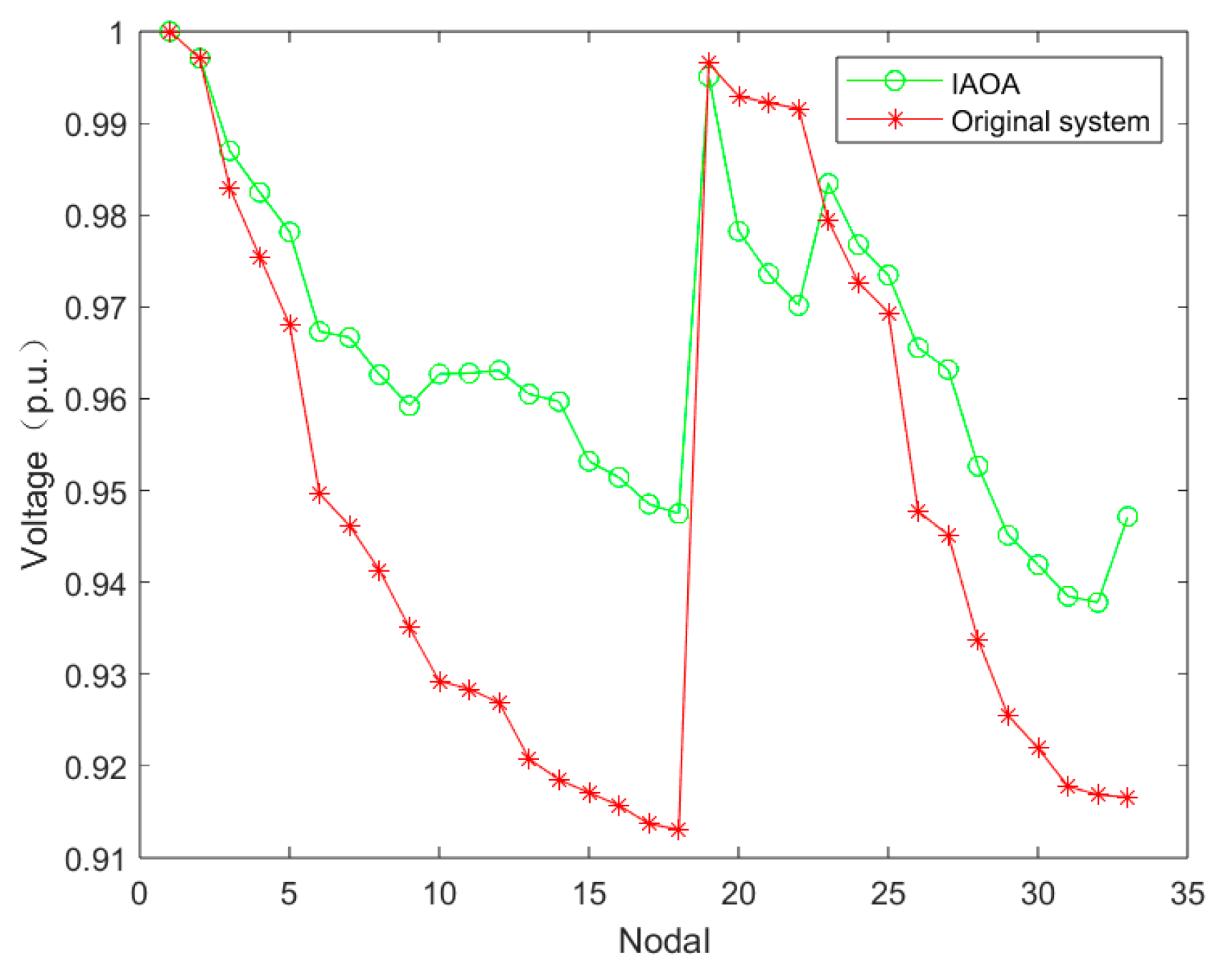
The IEEE33 node system has 32 branch circuits and 5 contact branch circuits, and in the initial state, the sectional switches of branch circuits 1–32 are closed, the contact switches of branch circuits 33–37 are disconnected, and the initial network loss in the system is 202.67 kW.

Table 3. IAOA distribution grid reconfiguration data of example 1.

Title 1	Before Refactoring	After Reconfiguration
Disconnected branch	B33, B34, B35, B36, B37	B7, B14, B9, B32, B37
System net loss/kW	202.68	139.55
Nodal voltage minimum/p.u.	0.91309	0.93787

shows the simulation results of the IAOA in the IEEE33 node system, which reveals that the system’s network loss decreases from 202.68 kW to 139.55 kW, with a decrease of about 31.13%. Figure 6 reflects the changes in the node voltages before and after reconfiguration, and the lowest node voltage rises from 0.91309 p.u. to 0.93787 p.u. Meanwhile, the distribution of the node voltages is more balanced and the quality of the system’s node voltages is significantly improved. As seen in Figure 7, both the AOA and IAOA can converge to the optimal solution after many iterations, but the ability of the IAOA to jump out of the local optimal solution and the convergence speed are significantly improved compared with the AOA.

5.2.2. Simulation Analysis of Example 2

The IEEE69 node system has 74 branches and 5 contact branches, and in the initial state, the sectional switches of branches 1–68 are closed, the contact switches of branches 69–73 are open, and the initial network loss in the system is 226.48 kW. The results of reconfiguration of the node system, through applying the IAOA, are shown in

Table 4. IAOA distribution grid reconfiguration data of example 2.

Title 1	Before Refactoring	After Reconfiguration
Disconnected branch	B69, B70, B71, B72, B73	B69, B70, B14, B50, B46
System net loss/kW	226.48	100.97
Nodal voltage minimum/p.u.	0.90893	0.94252

, and the system network loss is reduced from 226.48 kW to 100.97 kW, which is a reduction of about 55.42%; as with the 33-node system, the quality of each node voltage of the 69-node system in Figure 8 is significantly improved, and the lowest node voltage is improved from 0.90892 p.u. to 0.94252 p.u. The ability of the IAOA to jump out of the local optimal solution and the convergence speed in Figure 9 are significantly better than those of the AOA.

5.2.3. Simulation Analysis of Example 3

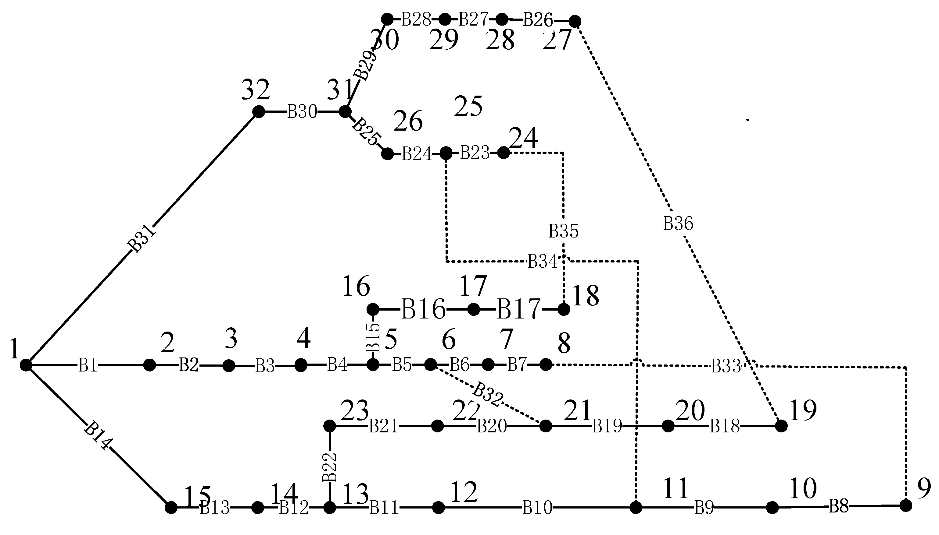
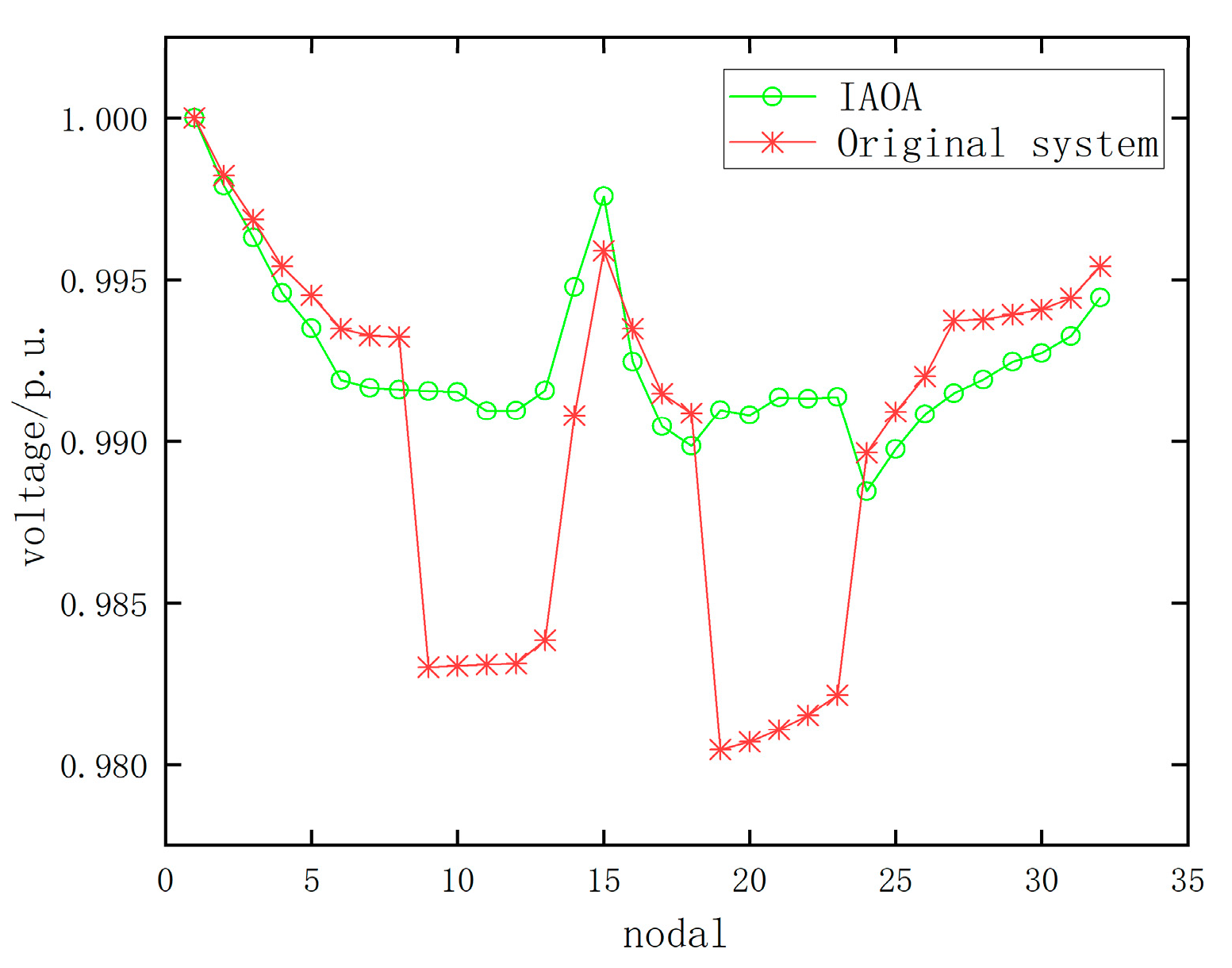
The proposed distribution network reconfiguration algorithm based on the IAOA in this paper demonstrates the superior performance of the algorithm in performing distribution network reconfiguration through the algorithmic performance testing and validation of Arithmetic Case 1 and Arithmetic Case 2. In addition, the simulation results of Example 1 and Example 2 also demonstrate the necessity of reconfiguration of distribution networks. To further validate the feasibility of the proposed algorithm and the practical engineering applicability of distribution network reconfiguration, simulation analysis is carried out in a real distribution network system, as shown in Figure 10. The system has 32 nodes, 31 branches, and 5 contact branches. In the initial state, the sectional switches of branches 1–31 are closed and the contact switches of branches 32–36 are open, and the initial network loss in the system is 91.37 kW. After the reconfiguration of this network system using the IAOA (the results are shown in

Table 5. Reconfiguration data for an actual network.

	Before Refactoring	After Reconfiguration
Disconnected branch	B32, B33, B34, B35, B36	B9, B19, B20, B34, B35
System net loss/kW	91.37	78.88
Nodal voltage minimum/p.u.	0.98265	0.98903

), the system network loss decreases from 91.37 to 78.88 kW, which is a reduction of about 13.67%. Figure 11 shows the changes in node voltage before and after reconfiguration. The lowest node voltage before reconfiguration occurs on node 19, and the lowest node voltage after reconfiguration occurs on node 24. The lowest node voltage increases from 0.98265 p.u. to 0.98903 p.u. The node voltage quality of the system is significantly improved and the distribution is more balanced.

6. Conclusions

In order to improve the optimization accuracy and convergence speed of the AOA, this paper adopted various hybrid strategies to improve it. The IAOA was proven to be an efficient optimization algorithm with high application value after comparison tests with the AOA, PSO, and SO. Subsequently, in the IEEE33 node system and IEEE69 node system, the distribution network was reconfigured based on the AOA and IAOA with the minimum network loss as the objective function, and the IAOA was shown to have fewer convergence iterations in reaching the optimal operating network structure. Finally, the IAOA was applied to a real distribution system, and the simulation results verified that the proposed algorithm can help to reconfigure the distribution network quickly; the network loss and node voltage of the system were significantly improved after the reconfiguration.

References

- Lin, C.-Y.; Xue, Y.-K.; Tseng, Y.-C. A review of distribution network reconfiguration research. Electr. Switchg. 2021, 59, 3–8. [Google Scholar]
- Alqahtani, M.; Marimuthu, P.; Moorthy, V.; Pangedaiah, B.; Reddy, C.R.; Kiran Kumar, M.; Khalid, M. Investigation and Minimization of Power Loss in Radial Distribution Network Using Gray Wolf Optimization. Energies 2023, 16, 4571. [Google Scholar] [CrossRef]
- Liao, F.; Chen, J.; Qu, W.; Wang, Y.; Hu, Y.; Wu, N. Active distribution network reconfiguration based on improved social spider algorithm. J. Power Syst. Autom. 2023, 35, 125–133. [Google Scholar]
- Wu, J.; Yu, Y. Multi-objective distribution network reconfiguration optimisation based on improved sum search algorithm. Power Syst. Prot. Control 2021, 49, 78–86. [Google Scholar]
- Merzoug, Y.; Abdelkrim, B.; Larbi, B. Distribution network recon-figuration for loss reduction using PSO method. Int. J. Electr. Comput. Eng. 2020, 10, 5009. [Google Scholar] [CrossRef]
- Wu, Y.; Liu, J.; Wang, L.; An, Y.; Zhang, X. Distribution Network Reconfiguration Using Chaotic Particle Swarm Chicken Swarm Fusion Optimization Algorithm. Energies 2023, 16, 7185. [Google Scholar] [CrossRef]
- Hong, Y.; Liu, T.; Fan, L.; Li, X. Reconfiguration of distribution networks containing distributed power sources based on immunogenetic algorithm. J. Power Syst. Autom. 2014, 26, 15–19. [Google Scholar]
- Jin, Y.; Zhang, L.; Wu, P.; Niu, Q.; Shen, Y. Application of improved genetic algorithm in reconfiguration of distribution network containing DG. Sens. Microsyst. 2020, 39, 153–156. [Google Scholar]
- Yang, M.; Liu, J. Distribution network reconfiguration based on genetic ant colony algorithm. Mod. Electron. Technol. 2020, 43, 128–132. [Google Scholar]
- Li, Z.; Zhang, Y.; Aqeel Ashraf, M. Optimization design of reconfiguration algorithm for high voltage power distribution network based on ant colony algorithm. Open Phys. 2018, 16, 1094–1106. [Google Scholar] [CrossRef]
- Abualigah, L.; Diabat, A.; Mirjalili, S.; Abd Elaziz, M.; Gandomi, A.H. The arithmetic optimization algorithm. Comput. Methods Appl. Mech. Eng. 2021, 376, 113609. [Google Scholar] [CrossRef]
- Zhang, W.; Li, S.; Qi, M.; Zhou, X.; Song, Y. Introduced a transitional phase and improvement of the gauss mutation arithmetic optimization algorithm. Small Microcomput. Syst. 2023, 1–12. Available online: http://kns.cnki.net/kcms/detail/21.1106.TP.20230413.1731.019.html (accessed on 3 February 2024).
- Zheng, T.; Liu, S.; Ye, X. Improved arithmetic optimization algorithm with adaptive t-distribution and dynamic boundary strategy. Comput. Appl. Res. 2022, 39, 1410–1414. [Google Scholar]
- Lan, Z.; He, Q. Multi-strategy fusion arithmetic optimization algorithm and its engineering optimization. Comput. Appl. Res. 2022, 39, 758–763. [Google Scholar]
- Abualigah, L.; Diabat, A.; Sumari, P.; Gandomi, A.H. A novel evolutionary arithmetic optimization algorithm for multilevel thresholding segmentation of COVID-19 CT images. Processes 2021, 9, 1155. [Google Scholar] [CrossRef]
- Wang, X.; Wang, R.; Wei, Y. Fault section location Method of Low Voltage Distribution Network based on Arithmetic Optimization Algorithm. Electron. Sci. Technol. 2023, 36, 25–31. [Google Scholar]
- Ding, B.; Kuang, Z.; Lu, L. Three-dimensional trajectory planning for UAVs based on Q-learning arithmetic optimization algorithm. Electro-Opt. Control 2024, 31, 61–69. [Google Scholar]
- Zheng, H.; Yu, J.; Yang, J.; Wei, S. Bat optimization algorithm based on cosine control factor and iterative local search. Comput. Sci. 2020, 47, 68–72. [Google Scholar]
- Zou, Y.; Wu, R.; Tian, X.; Li, H. Realizing the Improvement of the Reliability and Efficiency of Intelligent Electricity Inspection: IAOA-BP Algorithm for Anomaly Detection. Energies 2023, 16, 3021. [Google Scholar] [CrossRef]
- Kuang, X.; Yang, B.; Ma, H.; Tang, W.; Xiao, H.; Chen, L. Multiple strategy to improve dung beetle optimization algorithm. Comput. Eng. 2024, 1–20. Available online: http://kns.cnki.net/kcms/detail/31.1289.TP.20240301.1635.007.html (accessed on 28 March 2024).
- Huang, Y.; Qian, X.; Song, W. An improved differential evolutionary algorithm based on the dual-archive population size adaptive method. Comput. Appl. 2024, 1–14. Available online: http://kns.cnki.net/kcms/detail/51.1307.TP.20240305.0850.002.html (accessed on 7 April 2024).
- Wei, J.; Chen, Y.; Yu, Y.; Chen, Y. Optimal Randomness in Swarm-Based Search. Mathematics 2019, 7, 828. [Google Scholar] [CrossRef]
- Wang, Y.; Wang, W.; Yang, Y.; Zhou, H. Multiple strategy fusion algorithm improved Marine predators and its engineering application. Comput. Integr. Manuf. Syst. 2023, 1–21. Available online: http://kns.cnki.net/kcms/detail/11.5946.TP.20230515.1111.008.html (accessed on 5 February 2024).
- Hashim, F.A.; Hussien, A.G. Snake optimizer: A novel meta-heuristic optimization algorithm. Knowl. Based Syst. 2022, 242, 108320. [Google Scholar] [CrossRef]
- Lee, J.O.; Kim, Y.S.; Jeon, J.H. Generic power flow algorithm for bipolar DC microgrids based on Newton–Raphson method. Int. J. Electr. Power Energy Syst. 2022, 142, 108357. [Google Scholar] [CrossRef]
- Wang, S.; Shao, Z. Complex affine Ybus Gaussian iterative interval tidal current algorithm considering DG operation uncertainty. Power Autom. Equip. 2017, 37, 38–44. [Google Scholar]
- Dong, Z.; Zhang, B.; Liu, K.; Ma, Y. New forward pushback generation trend calculation method for active distribution networks. J. Power Syst. Autom. 2019, 31, 101–107. [Google Scholar]
Figure 1.
Comparison of the CMOA and MOA.
Figure 2.
Flowchart of the IAOA.
Figure 3.
Radial distribution network line diagram.
Figure 4.
IEEE33 node system diagram.
Figure 5.
IEEE69 node system diagram.
Figure 6.
Voltage distribution of 33 nodes before and after reconfiguration.
Figure 7.
Comparison of the AOA and IAOA’s convergence curves.
Figure 8.
Voltage distribution of 69 nodes before and after reconfiguration.
Figure 9.
Comparison of the AOA and IAOA convergence curves.
Figure 10.
Network structure of an actual power distribution system.
Figure 11.
Nodal voltage distribution of the actual distribution system after reconfiguration.