

Operational Robustness Assessment of the Hydro-Based Hybrid Generation System under Deep Uncertainties

State Key Laboratory of Eco-Hydraulics in Northwest Arid Region of China, Xi’an University of Technology, Xi’an 710048, China
*
Author to whom correspondence should be addressed.
Energies 2024, 17(8), 1974; https://doi.org/10.3390/en17081974
Submission received: 8 March 2024
/
Revised: 2 April 2024
/
Accepted: 9 April 2024
/
Published: 22 April 2024
(This article belongs to the Topic Advances in Renewable Energy Technologies and Systems Solutions)
Abstract
:The renewable-dominant hybrid generation systems (HGSs) are increasingly important to the electric power system worldwide. However, influenced by uncertain meteorological factors, the operational robustness of HGSs must be evaluated to inform the associated decision-making. Additionally, the main factors affecting the HGS’s robustness should be urgently identified under deep uncertainties, as this provides valuable guidance for HGS capacity configuration. In this paper, a multivariate stochastic simulation method is developed and used to generate uncertain resource scenarios of runoff, photovoltaic power, and wind power. Subsequently, a long-term stochastic optimization model of the HGS is employed to derive the optimal operating rules. Finally, these operating rules are used to simulate the long-term operation of an HGS, and the results are used to evaluate the HGS’s robustness and identify its main sensitivities. A clean energy base located in the Upper Yellow River Basin, China, is selected as a case study. The results show that the HGS achieves greater operational robustness than an individual hydropower system, and the robustness becomes weaker as the total capacity of photovoltaic and wind power increases. Additionally, the operational robustness of the HGS is found to be more sensitive to the total capacity than to the capacity ratio between photovoltaic and wind power.
1. Introduction
To address the problems posed by a warming climate, governments worldwide are focusing on carbon reduction targets and the transition to a low-carbon economy [1,2]. According to the “World Energy Outlook 2023” report published by the International Energy Agency, carbon emissions from the power sector account for over 40% of total global emissions. Therefore, building renewable dominant power systems is an important pathway to ensuring future energy security and mitigating climate change [3]. In this context, renewable energy such as photovoltaic (PV) and wind power are experiencing rapid growth. However, the non-dispatchability, fluctuations, and randomness of PV and wind power pose threats to the security of the power grid [4,5]. To ensure the safety and efficiency of electric power systems, there has been considerable research on the integration of hydropower, which has strong regulating capabilities, with PV and wind power to develop a hybrid generation system (HGS) [6,7,8]. In this way, the rapid regulatory capabilities of hydropower and renewable energy production potential can be fully utilized [9,10].
Many previous studies have proved that the stationarity of meteorological variables such as precipitation, temperature, radiation, humidity, and wind speed may be destroyed as an effect of climate change [11,12,13]. The operational management and capacity planning of HGSs may be affected by these meteorological factors, constituting deep uncertainties. To inform robust decision-making and capacity configuration, the impacts of these deep uncertainties on HGSs has been explored in several studies. François et al. (2018) [14] revealed the sensitivity of renewable energy penetration to climate change based on the Global Circulation Models (GCMs), for a solar/hydropower-dominated electric system. Perera et al. (2020) [15] indicated that the potential for integrating renewable energy into the power grid is greatly influenced by climate change under uncertain scenarios, considering both low impact variations and extreme events. These findings have motivated researchers to derive climate-resilient operating rules and planning strategies for the HGSs [16]. A two-stage adaptive robust optimization approach was proposed for a wind and pumped storage hybrid system, has been proposed to deal with the wind uncertainty [17], and a multi-stage robust scheduling method that maximizes the utilization of hydropower reserves has been developed to deal with the inflow uncertainty of a hydro-PV-wind hybrid system [18]. Overall, most studies consider to the sensitivity of the HGS to resource uncertainty, including our previous work [19]. However, exploring the sensitivity to the capacity configuration of the HGS itself would provide additional valuable guidance during the planning stage.
When evaluating the uncertainty of runoff, wind, and PV power resources, GCMs are commonly employed [20,21,22]. GCMs simulate global-scale climate variables under various carbon emission scenarios and models and subsequently obtain time series of regional climate factors through downscaling methods. These are then combined with hydrological models and other underlying surface factors to derive runoff series, and they are integrated with energy calculation models to determine wind and PV power output series [23]. However, existing studies have demonstrated the limitations of GCMs in simulating the most sensitive climate variables for water resources, such as relative humidity and precipitation [23,24]. Additionally, GCM data contain uncertainties, and as a top-down simulation method, propagate multiple sources of uncertainty (including downscaling model uncertainty, hydrological model uncertainty, and energy model uncertainty) to the runoff, PV and wind power series, resulting in suboptimal simulations [23,24]. To overcome the shortcomings of GCMs in assessing the robustness of HGSs, represented by changes in the runoff, PV, and wind power series [24]. Specifically, this study utilizes a multivariate stochastic simulation method to generate uncertain runoff, PV, and wind power scenarios.
This study is an extension of our previous work on the robustness of HGSs under uncertainty. The contributions of this study can be summarized as follows: (1) The factors affecting the sensitivity of the HGS to uncertain inputs are identified from among the various resource factors and capacity factors; and (2) a refined long-term stochastic dynamic programming model considering short-term characteristics is developed and used to derive the optimal operating rules for an HGS.
The remainder of this paper is arranged as follows. Section 2 introduces the methods used for model development, before Section 3 describes a case study and its corresponding parameters and data sources. Section 4 presents and discusses the results, and Section 5 summarizes the conclusions from this study.
2. Methods
First, a large set of uncertain scenarios concerning runoff, wind power, and PV resources are generated based on multivariate stochastic simulations, which is a bottom-up sequential simulation approach (see Section 2.1). Subsequently, a long-term optimization model for an HGS is constructed. Under the historical baseline state, the model is solved using stochastic dynamic programming (SDP) to generate long-term operating rules for the HGS (see Section 2.2). Next, the generated operating rules are simulated under uncertain runoff, PV, and wind power scenarios, and various robustness indicators are statistically evaluated based on the simulated scheduling results. Finally, sensitivity analysis is employed to determine the factors affecting the robustness of the HGS (see Section 2.3).
2.1. Multivariate Stochastic Simulation
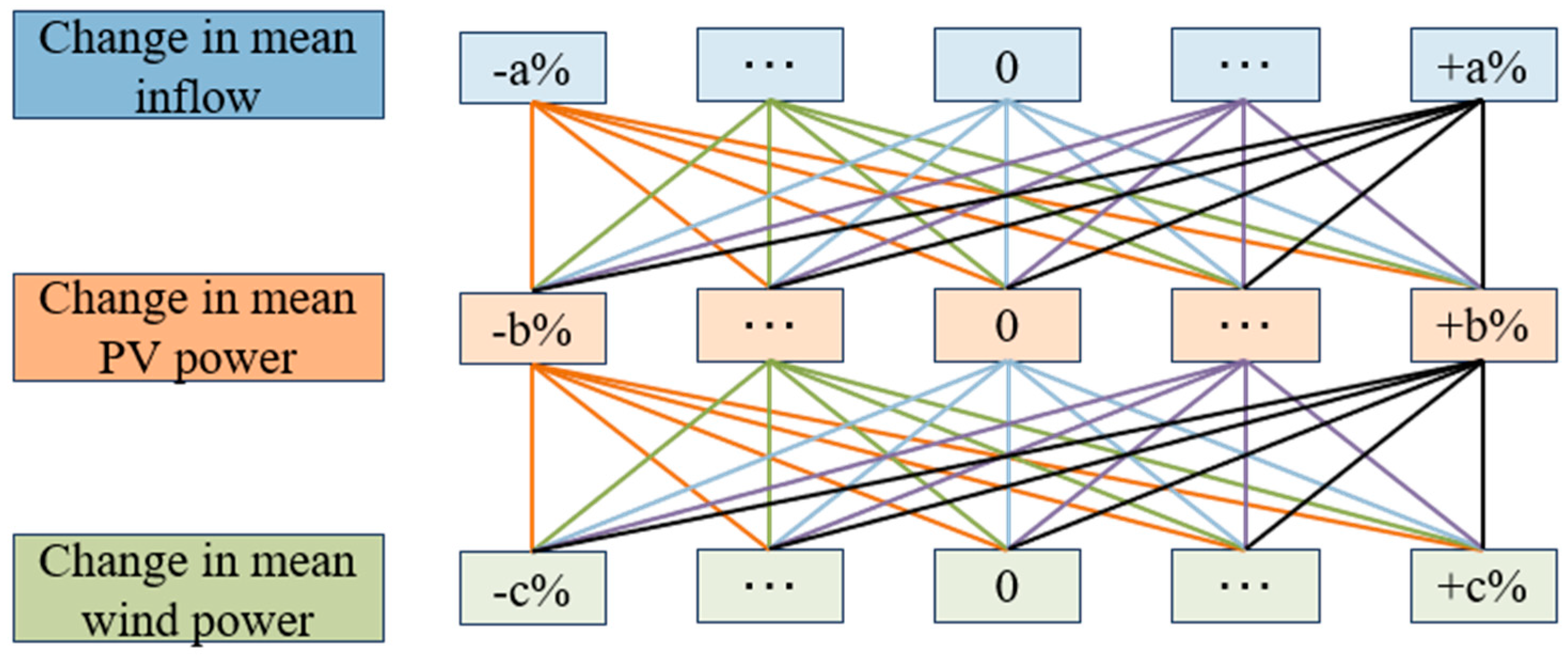
As a bottom-up simulation approach, the multivariate stochastic simulation method considers a range of the reservoir inflow, PV, and wind power. The change rate are all set to ±a%, ±b%, ±c%. Subsequently, the seasonal autoregressive (SAR) model based on the scaled inflow series was used to obtain the uncertain inflow scenarios. Copula functions are then used to construct joint probability distributions between the inflow series and PV/wind power output series. By using the joint probability distributions and Latin hypercube sampling (LHS) [25,26], the uncertain PV and wind power scenarios are simulated. Finally, the simulated inflow, PV, and wind power series are combined to generate a large number of uncertain scenarios (see Figure 1).
The detailed steps for generating the runoff, PV, and wind output series are as follows:
Step 1: The uncertain scenarios of the runoff are simulated as follows:
First, the historical runoff series is scaled according to its mean within the range of [−a%, a%], at intervals of 1%. Subsequently, an SAR model is constructed based on the scaled runoff series, with the model order determined using the Akaike’s information criterion and the model parameters determined using the least squares method. This model is used to simulate uncertain runoff series, represented by . To ensure the representativeness of uncertain scenarios and mitigate errors introduced by random sampling, the simulation period is set to 1000 years.
Step 2: The change rates of historical runoff and PV/wind power output are all set as [−10%, 10%] in this work, and their time series are scaled as follows:
where and are the scaled inflow and PV/wind power output series, respectively; and denote the historical inflow and PV/wind power output series, respectively; a and b are the scaling parameters of the inflow and PV/wind power output series, respectively.
Step 3: The joint probability distribution is constructed as follows:
First, eight theoretical probability distribution functions including the extreme value distribution, exponential distribution, gamma distribution, general extreme value distribution, general Pareto distribution, lognormal distribution, normal distribution, and Weibull distribution are selected. These distributions are used to individually fit probability distributions for and . Akaike’s information criterion is utilized to assess the disparities between the theoretical probability distributions and the empirical probability distributions under different functional forms [27]. The optimal theoretical probability distribution form and parameters are then selected as the marginal probability distributions for the joint probability distribution.
Three Archimedean Copula functions are then used to construct the joint probability distribution functions for and represented as , , and ; a detailed expressions can be found in previous studies [27,28]. The optimal form and parameters of the joint probability distribution function are then selected using the Squared Euclidean distance [29]. In this approach, the disparities between the theoretical Copula and empirical Copula are represented by the distance value d, with smaller values of d indicating a more appropriate Copula function.
, , and are the joint probabilities of and given by the three forms of Copula functions; denotes probability density of ; represents the probability density of ; and is the parameter of the joint probability distribution.
Step 4: The uncertain scenarios of the PV/wind power output are simulated as follows:
The probability of the PV/wind output series under runoff , is denoted as . It is assumed that the joint probability distribution function between and remains consistent with the joint probability distribution function between and . Subsequently, LHS is used to generate a sequence of random numbers p is generated, and the Copula conditional probability is equals to p. Here, can be expressed as a function of the marginal distributions us and vs, using Equations (2)–(4). Then, based on the probability density function us of the series, parameters of the joint probability distribution function, and , the expression functions (Equations (2)–(4)) are solved to obtain the probability density function of the series. Finally, the marginal probability distribution function vs is used to calculate by solving the inverse expression function of vs.
2.2. Long-Term Optimization Model Considering Intraday Electricity Curtailment of the HGS
2.2.1. Objectives of the Long-Term Operation Model
The time interval of the long-term operation model is commonly set to one month or ten days, making it difficult to consider the intraday electricity curtailment of PV and wind power. As a result, the power generation performance of HGSs is often overestimated. To overcome this issue, the response function characterizing the long-term power decision and the short-term electricity curtailment performance is used to quantify the electricity curtailment in the long-term operation model. In this study, the two model objectives are to maximize the energy production and maximize the guaranteed rate.
Objective 1: maximize energy production
Objective 2: maximize the guaranteed rate
where denotes the total energy production of the HGS; indicates the system’s power output at the t period; is the firm output of the HGS; is the hydropower output of the m-th cascade hydropower plants at the t period; and denote the PV and wind power output at the t period, respectively. is the electricity response function; detailed steps for generating this function can be seen in our previous study [30]; represents the time interval during one operational period; denotes the guaranteed rate of the HGS; indicates the number of operational periods that the HGS’s total output equals or exceeds .
In this study, a penalty function method was used to simplify the multi-objective model into one-objective model. The objectives integrated with the penalty function can be expressed in the form:
where is the penalty function; equals 108.
The constraints in this operation model are the mass balance constraint, reservoir characteristic constraint, power generation constraint, and power transmission constraint.
2.2.2. Solving Method
As the aim of this study is to assess the robustness of the water and wind complementary system under uncertain scenarios, it is appropriate to use uncertain model inputs rather than deterministic historical data series to derive the operating rules. Therefore, SDP is employed to solve the long-term optimization mode. In SDP, the uncertainty of the model input series is represented by a discrete characteristic value based on a probability distribution function [31].
In this study, the reservoir water level is used as the state variable for the operation model. To accommodate uncertain inputs, the inflow, PV, and wind power outputs are integrated as additional state variables in the recursive equation of the SDP. The decision variable (final reservoir level in the operational period) can be expressed as a function of the state variables (reservoir capacity, inflow, PV, and wind power output) as follows:
where and denote the final and initial water levels in period t; represents the reservoir’s inflow in period t.
In the SDP method, the key step is to determine the formulation of the recursive equation, used to characterize the transition principles of the system states between adjacent operational periods. In this study, the runoff and PV/wind power output are assumed to be correlated. The recursive equation for the operation model considering the relationship between the inflow and PV/wind power can be expressed as follows:
where Et(•) denotes the expected energy production of the HGS from operational period t to the end of the production term; Bt(•) represents the system’s total energy production during period t; indicates the i-th discrete characteristic value in the period t; is the probability of the state variable transitioning from discrete state i to discrete state j as the time changes from period t to period t + 1.
2.3. Robustness Indicators
To assess the performance of the proposed model, three indicators are used to evaluate the robustness of the HGS:
- (1)
- Improved regret-based indicator Rm
Rm is defined as the maximum deviation from the baseline state under uncertain conditions, and is expressed as follows:
where denotes the i-th technical/economic indicators in the j-th uncertain scenario; represents the i-th technical/economic indicators in the historical baseline state; represents the difference between and . The value of Rm lies between 0 and 1, with values closer to 0 indicating the stronger robustness of the HGS. Technical and economic indicators contain the monthly average spilled water, hydropower generation, total energy production, guaranteed rate, and electricity curtailment indicators.
- (2)
- Satisfied-based indicator S1
The satisfied-based indicator S1 is defined as the average level at which all technical/economic indicators of the HGS meet the stakeholders’ requirements under uncertain scenarios. The expression is as follows:
where indicates that all technical/economic indicators of the HGS under the j-th uncertain scenario satisfy the stakeholders’ requirement; In contrast, indicates the requirement cannot be met. N represents the number of uncertain scenarios.
- (3)
- Satisfied-based indicator S2
The satisfied-based indicator S2 is defined as the uncertainty horizon without the system’s minimum requirement being missed [32]. The expression is as follows:
where is the number of uncertain scenarios in which the HGS achieves its minimum requirement. In this study, HGS’s minimum requirement is defined as when the system’s power guaranteed rate exceeds 90%, indicating that is set as 0.9.
2.4. Sensitivity Analysis of HGS Robustness
The two main factors influencing HGS robustness are the time series of model inputs (such as inflow, PV, and wind) and the installed capacity structure of the HGS. In terms of the former, the uncertainties in the resource time series have been considered when simulating the uncertain scenarios. Hence, the sensitivity analysis of these three factors involves obtaining and analyzing the system’s robustness under each scenario, and the performance is reflected by S1j and S2j. In terms of the latter, the system’s installed capacity structure can be divided into two factors: the total installed capacity of PV and wind, and the capacity ratio between PV and wind (the capacity of the cascade hydropower plants is predetermined). A global sensitivity analysis is applied to identify the main factor affecting system robustness.
Global sensitivity analysis primarily quantifies the relative contributions of the input variables, model parameters, and model structure uncertainties to the variations in output [33]. The aim is to assess the robustness of model outputs to various sources of uncertainty by quantifying the influence of different factors. Variance-based sensitivity analysis is commonly used to quantify the sensitivity of the model under uncertain conditions. The capacity ratio and the total installed capacity of PV and wind power are considered as the two sensitive factors, and the three robustness indicators are set as the model outputs. The variance of these indicators under the uncertain scenarios is statistically analyzed to assess the robustness of the HGS. The sensitivity of the HGS to each factor can be expressed as follows:
where , , and denote the sensitivity of the HGS’s robustness to the factors, when robustness is represented by Rm, S1, and S2, respectively; us indicates the uncertain scenario of the capacity ratio and total installed capacity of the PV and wind power plants.
3. Case Study
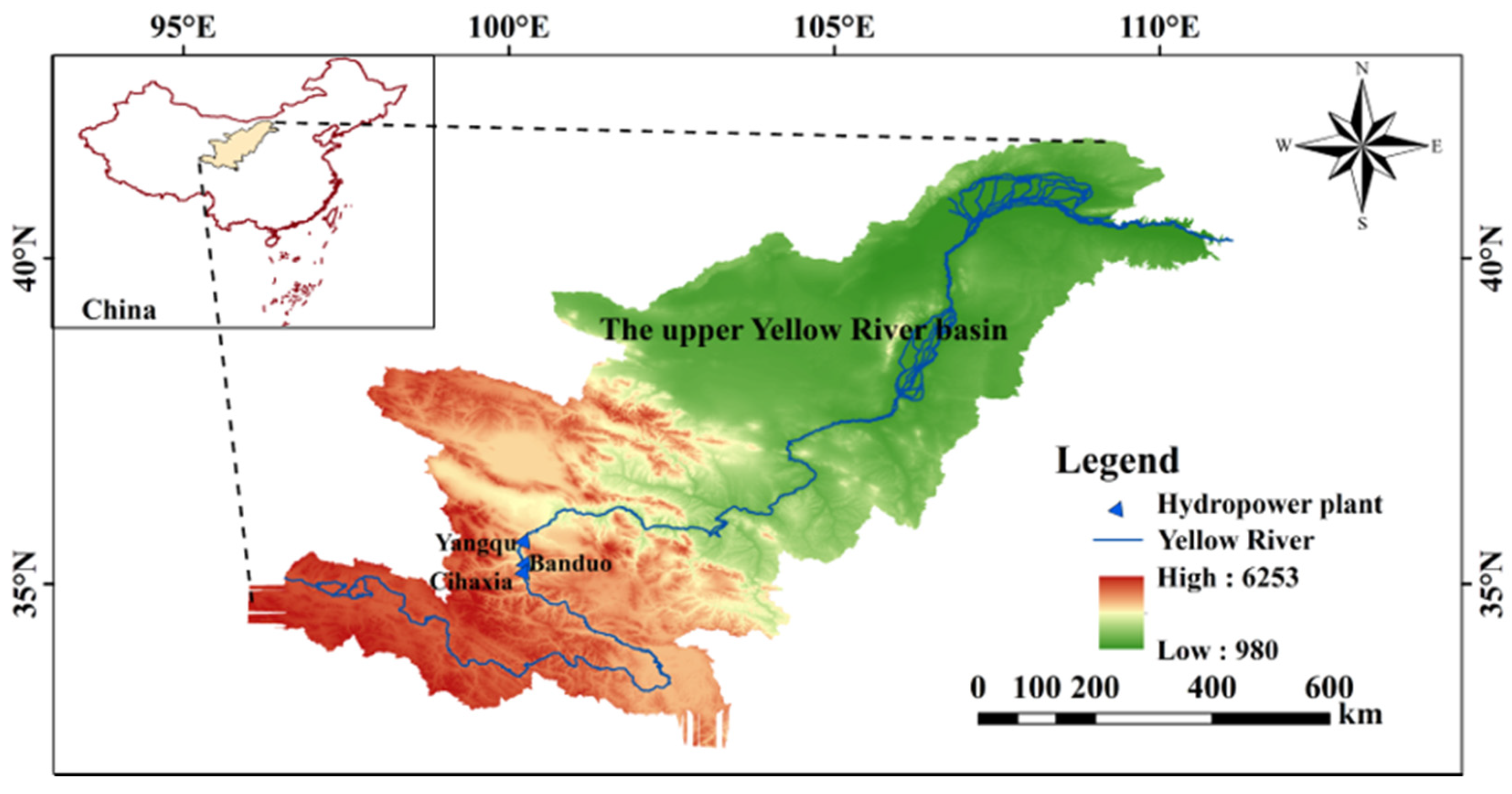
The clean energy base located in the Upper Yellow River Basin, China, was selected for a case study. This region contains three cascade hydropower plants: Cihaxia, Banduo, and Yangqu, as well as nearby PV power plants (1-Tala and 3-Tala) and wind power plants (Qieji and 2-Tala). The Cihaxia reservoir operates with seasonal regulation ability, whereas Banduo and Yangqu operate with daily regulation ability. The locations of these clean energy bases are shown in Figure 2. The main parameters of the cascade hydropower plants are summarized in Table 1.
The monthly inflow series of the cascade reservoirs, ranging from January 1959 to December 2019,were obtained from the Yellow River Conservancy Commission. The monthly PV and wind power output series were calculated using PV energy and wind energy models based on the monthly sunshine duration, air temperature, and wind speed time series [34]. These meteorological time series were obtained from the China Meteorological Administration.
All optimization programs were implemented with Matlab2019a (https://www.mathworks.com/) on a PC with Intel(R) Core(TM) i5-12600K CPU, 16.00 GB of RAM.
4. Results and Discussion
4.1. Simulation Results of the Inflow, PV, and Wind Power Series
Three cascade hydropower plants were considered in this study: Cihaxia, Banduo, and Yangqu, from upstream to downstream. Uncertain scenarios concerning the inflow series of Cihaxia, the interval inflow between Cihaxia and Banduo, and the interval inflow between Banduo and Yangqu were simulated based on the SAR model. Assuming a variation range of [−10%, 10%] about the mean of the inflow series, 21 uncertain scenarios were generated at intervals of 1%. The simulation results are shown in Figure 3.
Figure 3 illustrates that compared with the historical inflow series, the distribution range of the simulated inflow has expanded, while still maintaining consistent statistical characteristics with the historical inflow series. The mean and variance are statistical features of the runoff time series, where an increase or decrease in the mean indicates an increase or decrease in the available storage of the reservoir. An increase in the variance suggests greater interannual fluctuations in the monthly reservoir inflow series. The simulated inflow series exhibits mean and variance parameters that are consistent with the historical inflow series in each month, thereby validating the rationality and effectiveness of the SAR model developed in this study.
Based on the proposed multivariate stochastic simulation method, the time series of PV/wind power was simulated under specific uncertainties. The PV/wind simulated time series under a −10% scenario with a −10% change in inflow conditions are shown in Figure 4.
Figure 4 indicates that compared with the historical time series of the PV and wind power output, the distribution range of the simulated PV and wind power output series has expanded, while still maintaining the consistent statistical characteristics with the historical series. This validated the effectiveness of the multivariate stochastic simulation method. Specifically, the variance parameter of the simulated wind power output is relatively larger from May to August compared with the historical series. This can be attributed to the higher interannual fluctuation observed in the monthly wind power output distribution. Although the installed capacity of wind power is only half that of PV power, the variance in wind power output reaches 3–5 times that of PV power during each month.
To verify the efficiency of the simulation results in all uncertain scenarios, the mean and standard deviation of the stochastic variables under historical and simulated conditions are compared in Table 2 and Table 3. The maximum deviation in the mean values is 2.5%, and that of the standard deviation is 4.7.
The variation ranges for the three resources were set as [−10%, 10%]. Therefore, by randomly combining the simulated uncertain scenarios of these three variables, a total of 21 × 21 × 21 = 9261 uncertain scenarios were obtained and used to assess the robustness of the HGS.
4.2. Long-Term Operation Results
To verify the effectiveness of the proposed long-term hydro–PV–wind complementary operation model (Scheme I), two other operation models for the Upper Yellow River Clean Energy Base were constructed for comparison: a long-term hydropower operation model (Scheme II) and a long-term operation model based on the standard operating policy (SOP) (Scheme III). In Scheme II, the objectives of the optimization model were set as the maximization of the hydropower generation and hydropower guaranteed rate, and the system’s total output equals the summary of the optimized hydropower output and the non-dispatchable PV/wind power output. The model’s constraints and solving method in Scheme II are consistent with those for Scheme I. In Scheme III, the long-term operation of the HGS is based on the SOP, with the operation decision made according to the available energy in each operational period [35]. The technical and economic indicators based on the operation results of the three schemes are exhibited in Figure 5.
Figure 5 shows that all indicators under Schemes I and II are better than those under Scheme III. Specifically, compared with Scheme III, the spilled water indicator decreases by 7.9% under Scheme I, while the average annual hydropower generation increases by 6.3%, the average annual total energy production increases by 7%, the average annual PV and wind power generation increases by 8.3%, the guaranteed rate increases by 32%, and electricity curtailment decreases by 6.9%. In addition, the average annual hydropower generation and total energy production of 162.37 × 10⁸ kWh and 254.02 × 10⁸ kWh, respectively [31], are close to the results obtained in this study. The operation results obtained in this study are slightly lower than those in the literature because the uncertainty time series were input into the long-term optimization model rather than using the deterministic model input. This policy results in more robust operating rules, albeit at the loss of system energy production. These findings verify the effectiveness and reliability of the proposed long-term optimization model.
The other evaluation indicators under Scheme are better than those under Scheme I. This reveals that Scheme II optimizes the storage and release rules falling down rules of the cascade hydropower stations, thus increasing the water head and maximize hydropower generation. In contrast, Scheme I focuses on the complementary regulation for PV and wind power to minimize the electricity curtailment rate. Hence, the hydropower generation indicator in Scheme I is slightly lower than those under Scheme II.
4.3. Robustness Assessment of the HGS
The operating rules derived from the long-term operation models under Schemes I and II were simulated using the uncertain scenarios. Based on the simulation results, three robustness indicators were calculated. The results are shown in Figure 6.
Figure 6 shows that all three robustness indicators indicate better robustness of the HGS under hydro–PV–wind complementary operation (Scheme I) compared to individual hydropower operation (Scheme II). Specifically, the regret-based indicator Rm and satisfied-based indicator S1 show relatively similar values under the two operation schemes, while the S2 indicator under Scheme I is significantly higher than that under Scheme II.
Rm and S1 indicators mainly characterize the robustness of the HGS considering the comprehensive technical and economic performance, whereas S2 emphasizes the robustness of power supply reliability. The results highlight that the hydro-PV-wind complementary operating rules significantly enhance the power supply reliability of the HGS under uncertain resource scenarios.
The robustness indicators were all calculated based on several technical and economic indicators. To further reveal the reasons for the improved robustness of Scheme I, we now analyze the technical and economic performance of the HGS under uncertain scenarios. The cumulative distributions of the technical and economic indicators under uncertain scenarios are presented in Figure 7.
Figure 7b shows that, in terms of the average annual total energy production, the cumulative probability distribution curves under both two schemes are close to overlapping; however, the probability of the system meeting the requirement (results under historical baseline state) of Scheme I is 66.85%, higher than that under Scheme I (65.89%). This is because the total energy production indicator covers a wide fluctuation range [233.2 × 10⁸ kWh, 278.6 × 10⁸ kWh] under the uncertain scenarios, and the range is larger than the energy production deviation between different operation schemes (0.5–1.5 × 10⁸ kWh). Therefore, the two curves in Figure 7b seem to be close.
Figure 7a,d show that cumulative distribution of the hydropower generation indicator and the spilled water indicator are stair-shaped. This is because both indicators are primarily influenced by the uncertainty in inflow, and are less affected by variations in PV and wind power. Therefore, under uncertain scenarios where the inflow series remains constant, while PV and wind power output change, both indicators remain relatively stable. In addition, the cumulative distribution curves under Scheme II exhibit strict stair-shaped patterns, whereas the shapes under Scheme I are approximately stair-shaped. This is due to the operation decision of the HGS under the hydropower operating rule that was made based on the reservoir water level and inflow stage and completely independent of the PV and wind power state. However, the hydropower output of the HGS under the complementary operating rule needs to compensate for the PV and wind power output, subsequently sacrificing partial hydropower generation production. Similar findings in the existing literature [36] verify the effectiveness of the results in this study. Hence, the cumulative distribution curves under Scheme I in Figure 7a,d are approximately stair-shaped.
Figure 7c,e show that, in terms of the guaranteed rate, the probability of achieving the requirement (under the historical baseline state) is 88.77% under Scheme I and 54.00% under Scheme II. Scheme I performs significantly better. In terms of the electricity curtailment rate, the probability of achieving the requirement is 100% under Scheme I and 11% under Scheme II. The hydro–PV–wind complementary operating rules produce markedly better performance.
In summary, the robustness of the HGS is more sensitive to the resource series than to the operation schemes. This study has evaluated the robustness of the HGS under various uncertain scenarios. To provide further guidance and advice on the capacity planning of the HGS, it is necessary to identify the key factors that influence system robustness. Therefore, the next subsection presents the results of a sensitivity analysis of the HGS.
4.4. Sensitivity Analysis of the HGS’s Robustness
Two sensitivity factors affecting the robustness of the HGS were analyzed under uncertain resource scenarios. The resource uncertainty includes uncertainties associated with inflow, PV, and wind power output factors. The capacity structure of the HGS considers the total capacity factor and capacity ratio factor of the PV and wind power plants.
4.4.1. Inflow PV and Wind Power Series Factors
The procedural variables S1j and S2j can be used to evaluate the system’s robustness in each uncertain scenario. As shown in Figure 8, S1j and S2j take values of (0, 1). A value of 0 indicates that the system cannot meet the robustness requirements under the j-th uncertain scenario, while a value of 1 indicates that the robustness requirements are satisfied. The robustness requirement of S1 is defined as the system’s hydropower generation, total energy production, guaranteed rate, spilled water, and electricity curtailment rate all exceeding those under the historical baseline state. The robustness requirement of S2 is defined as the power generation guaranteed rate of the system exceeding 90% under the uncertain scenarios.
Figure 8a reveals that when the runoff variation exceeds 2%, S1i always equals 1, indicating that the robust requirement can always be met. Conversely, when the runoff variation is less than −7%, S1i is always equal to 0, indicating the requirement cannot be met. When under the range of [−7%, 2%], S1i may equal 0 or 1, depending on the changing scenario of PV power. Hence, the changing range of [−7%, 2%] can be used to quantify the sensitivity of the HGS’s robustness to the inflow uncertainty. In terms of the ordinate of Figure 8a, the changing range of PV power significantly exceeds the [−10%, 10%]. A smaller changing rage indicates stronger sensitivity. Therefore, HGS’s robustness is more sensitive to inflow based on the satisfied-based indicator S1.
A similar analysis was extended to Figure 8b–f, and the results indicate that, when the satisfied-based indicator S1 was applied to quantify the HGS’s robustness, the robustness is most sensitive to inflow variation, followed by PV power variation and wind power variation. In addition, when the satisfied-based indicator S2 was applied to quantify the HGS’s robustness, the robustness is most sensitive to changes in the PV power output, followed by inflow variation and wind power variation.
4.4.2. Total Capacity and Capacity Ratio Factors
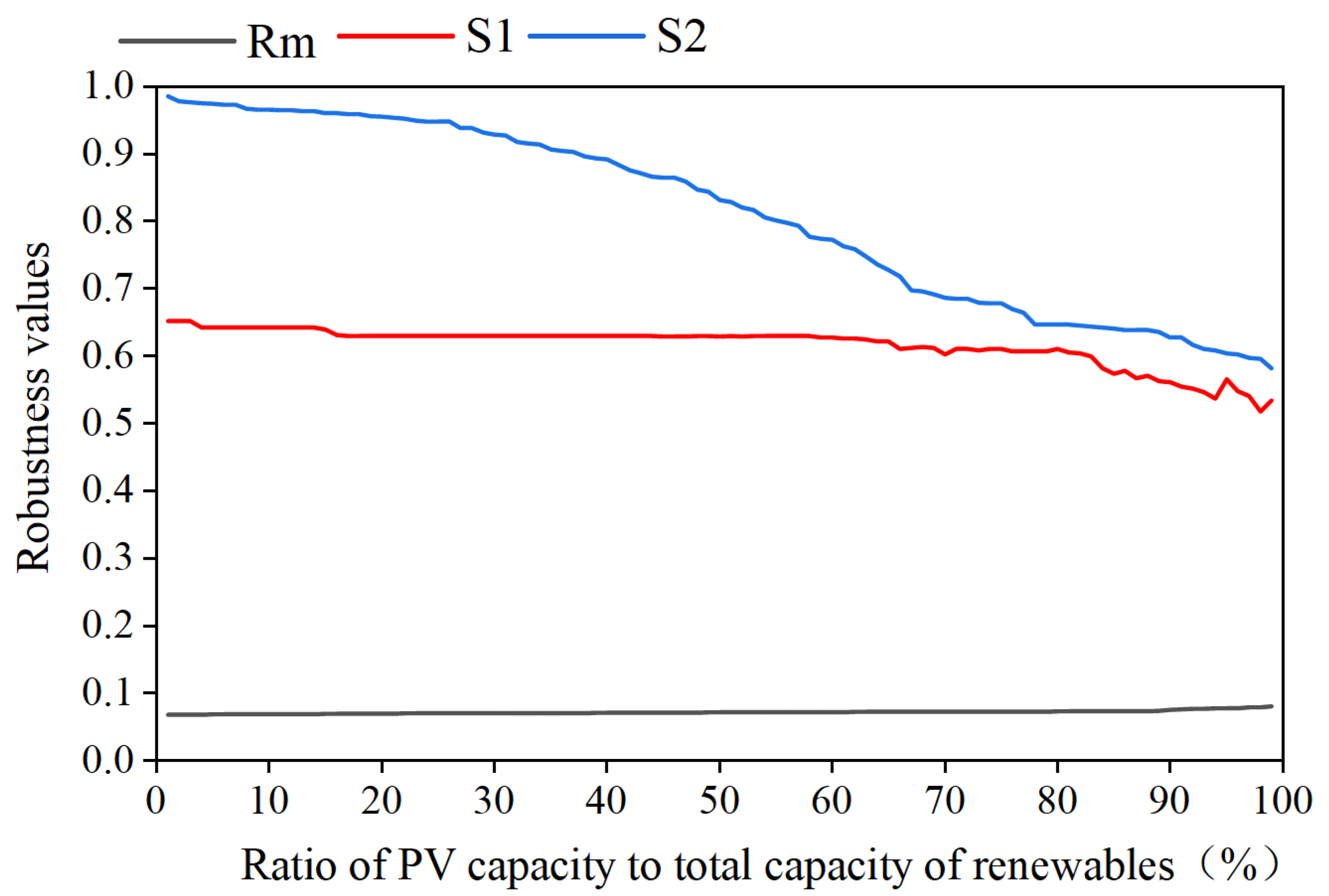
The robustness indicators for the HGS under variations in the installed capacity and capacity ratio of PV and wind power are exhibited in Figure 9 and Figure 10, respectively.
Figure 9 illustrates that, as the installed capacity of PV and wind power plants increase, the regret-based Rm continuously increases (smaller values indicate better robustness), while S1 and S2 decrease (larger values indicate greater robustness). These findings reveal that the HGS’s robustness weakens as the PV and wind power capacity increase.
Figure 10 shows that, when the PV capacity ratio (counting the total capacity of PV and wind power) is less than 30%, all robustness indicators reveal that the HGS can maintain stable robustness. When the PV capacity ratio is greater than 30% but less than 85%, the satisfied-based S2 indicates a significant decrease in the performance and in the power supply reliability of the HGS. When the PV capacity ratio exceeds 85%, all indicators point to a decline in the comprehensive robustness performance of the HGS.
The variance-based sensitivity indicators of HGS robustness, corresponding to the installed capacity and capacity ratio of PV and wind power, are summarized in Table 4. The findings reveal that the HGS’s robustness is more sensitive to the total installed capacity than the capacity ratio of PV and wind power.
5. Conclusions and Prospects
To evaluate the robustness of HGSs under inflow, PV, and wind power uncertainties, a multivariate stochastic simulation method was developed to generate a large set of uncertain scenarios. Subsequently, a long-term optimization model for an HGS was constructed and solved based on SDP, allowing us to derive operating rules under the historical baseline state. The generated operating rules were then simulated under uncertain scenarios concerning runoff, PV, and wind power. Finally, the operation results were used to evaluate the robustness of the HGS and identify its most sensitive factors. The main conclusions from this study are as follows:
- (1)
- Long-term hydro-PV-wind complementary operation can significantly enhance the technical and economic performance in the historical state and the system’s robustness under uncertain resource scenarios, albeit by sacrificing hydropower generation performance.
- (2)
- When the robustness of the HGS is considered in terms of the comprehensive complementary performance, there is higher sensitivity to changes in inflow, followed by variations in PV and wind power. However, when the power supply reliability is the primary focus, the HGS is most sensitive to changes in PV power.
- (3)
- The HGS’s robustness weakens as the total capacity of PV and wind power plants increases. Moreover, the robustness is initially unchanged before becoming weaker as the PV capacity ratio increases. Notably, the robustness of the HGS demonstrates higher sensitivity to changes in the total capacity than to changes in the capacity ratio.
In the present study, the mean changes in stochastic variables were assumed to cover a specific range. However, future climate change may alter the variability (e.g., variance and extreme values) of these stochastic variables. Therefore, accurate characterization of multiple uncertain inputs to the energy system under climatic changes should be considered in the planning, management, and evaluation of energy systems. Although GCM data can be used to project future hydrometeorological variables, they can only provide a small number of uncertainty scenarios and are hardly able to support the robustness evaluation. Hence, the multivariate stochastic simulation method will be combined with GCM data in future work. In addition, the proposed robustness evaluation framework will be extended to other energy bases.
Author Contributions
Conceptualization, J.J. and B.M.; methodology, J.J. and B.M.; software, J.J.; validation, J.J., B.M. and Q.H.; formal analysis, J.J.; investigation, J.J.; resources, B.M.; data curation, J.J.; writing—original draft preparation, J.J.; writing—review and editing, B.M.; visualization, J.J.; supervision, Q.B.; project administration, Q.H.; funding acquisition, B.M. All authors have read and agreed to the published version of the manuscript.
Funding
This study was supported by the “National Natural Science Foundation of China” [grant numbers U2243216, 52379023], the “Postdoctoral Innovative Talent Foundation of China” [grant number BX20200276], the “Postdoctoral Science Foundation of China” [grant number 2020M673453], and the “Doctoral Dissertation Innovation Fund of Xi’an University of Technology” [grant number 310-252072211].
Data Availability Statement
The original contributions presented in the study are included in the article, further inquiries can be directed to the corresponding authors.
Conflicts of Interest
The authors declare no conflict of interest.
References
- Brockway, P.E.; Owen, A.; Brand-Correa, L.I.; Hardt, L. Estimation of Global Final-Stage Energy-Return-on-Investment for Fossil Fuels with Comparison to Renewable Energy Sources. Nat. Energy 2019, 4, 612–621. [Google Scholar] [CrossRef]
- Yang, S.; Fang, D.; Chen, B. Human Health Impact and Economic Effect for PM2.5 Exposure in Typical Cities. Appl. Energy 2019, 249, 316–325. [Google Scholar] [CrossRef]
- Canales, F.A.; Jurasz, J.; Beluco, A.; Kies, A. Assessing Temporal Complementarity between Three Variable Energy Sources through Correlation and Compromise Programming. Energy 2020, 192, 116637. [Google Scholar] [CrossRef]
- Ma, X.Y.; Sun, Y.Z.; Fang, H.L. Scenario Generation of Wind Power Based on Statistical Uncertainty and Variability. IEEE Trans. Sustain. Energy 2013, 4, 894–904. [Google Scholar] [CrossRef]
- Ma, C.; Xu, X.; Pang, X.; Li, X.; Zhang, P.; Liu, L. Scenario-Based Ultra-Short-Term Rolling Optimal Operation of a Photovoltaic-Energy Storage System under Forecast Uncertainty. Appl. Energy 2024, 356, 122425. [Google Scholar] [CrossRef]
- Ávila, L.; Mine, M.R.M.; Kaviski, E.; Detzel, D.H.M. Evaluation of Hydro-Wind Complementarity in the Medium-Term Planning of Electrical Power Systems by Joint Simulation of Periodic Streamflow and Wind Speed Time Series: A Brazilian Case Study. Renew. Energy 2021, 167, 685–699. [Google Scholar] [CrossRef]
- Xu, B.; Zhu, F.; Zhong, P.-a.; Chen, J.; Liu, W.; Ma, Y.; Guo, L.; Deng, X. Identifying Long-Term Effects of Using Hydropower to Complement Wind Power Uncertainty through Stochastic Programming. Appl. Energy 2019, 253, 113535. [Google Scholar] [CrossRef]
- Ding, Z.; Wen, X.; Tan, Q.; Yang, T.; Fang, G.; Lei, X.; Zhang, Y.; Wang, H. A Forecast-Driven Decision-Making Model for Long-Term Operation of a Hydro-Wind-Photovoltaic Hybrid System. Appl. Energy 2021, 291, 116820. [Google Scholar] [CrossRef]
- Yuan, W.; Wang, X.; Su, C.; Cheng, C.; Liu, Z.; Wu, Z. Stochastic Optimization Model for the Short-Term Joint Operation of Photovoltaic Power and Hydropower Plants Based on Chance-Constrained Programming. Energy 2021, 222, 119996. [Google Scholar] [CrossRef]
- Zhu, F.; Zhong, P.-A.; Xu, B.; Liu, W.; Wang, W.; Sun, Y.; Chen, J.; Li, J. Short-Term Stochastic Optimization of a Hydro-Wind-Photovoltaic Hybrid System under Multiple Uncertainties. Energy Convers. Manag. 2020, 214, 112902. [Google Scholar] [CrossRef]
- Steffen, W.; Richardson, K.; Rockström, J.; Cornell, S.E.; Fetzer, I.; Bennett, E.M.; Biggs, R.; Carpenter, S.R.; De Vries, W.; De Wit, C.A.; et al. Planetary Boundaries: Guiding Human Development on a Changing Planet. Science 2015, 347, 736–746. [Google Scholar] [CrossRef] [PubMed]
- Scholze, M.; Knorr, W.; Arnell, N.W.; Prentice, I.C. A Climate-Change Risk Analysis for World Ecosystems. Proc. Natl. Acad. Sci. USA 2006, 103, 13116–13120. [Google Scholar] [CrossRef] [PubMed]
- Walther, G.R.; Post, E.; Convey, P.; Menzel, A.; Parmesan, C.; Beebee, T.J.C.; Fromentin, J.M.; Hoegh-Guldberg, O.; Bairlein, F. Ecological Responses to Recent Climate Change. Nature 2002, 416, 389–395. [Google Scholar] [CrossRef] [PubMed]
- François, B.; Hingray, B.; Borga, M.; Zoccatelli, D.; Brown, C.; Creutin, J.D. Impact of Climate Change on Combined Solar and Run-of-River Power in Northern Italy. Energies 2018, 11, 290. [Google Scholar] [CrossRef]
- Perera, A.T.D.; Javanroodi, K.; Nik, V.M. Climate Resilient Interconnected Infrastructure: Co-Optimization of Energy Systems and Urban Morphology. Appl. Energy 2021, 285, 116430. [Google Scholar] [CrossRef]
- Nik, V.M.; Perera, A.T.D.; Chen, D. Towards Climate Resilient Urban Energy Systems: A Review. Natl. Sci. Rev. 2021, 8, nwaa134. [Google Scholar] [CrossRef] [PubMed]
- Jin, X.; Liu, B.; Liao, S.; Cheng, C.; Zhang, Y.; Zhao, Z.; Lu, J. Wasserstein Metric-Based Two-Stage Distributionally Robust Optimization Model for Optimal Daily Peak Shaving Dispatch of Cascade Hydroplants under Renewa-ble Energy Uncertainties. Energy 2022, 260, 125107. [Google Scholar] [CrossRef]
- Zhou, Y.; Zhao, J.; Zhai, Q. 100% Renewable Energy: A Multi-Stage Robust Scheduling Approach for Cascade Hydropower System with Wind and Photovoltaic Power. Appl. Energy 2021, 301, 117441. [Google Scholar] [CrossRef]
- Jiang, J.; Ming, B.; Huang, Q.; Chang, J.; Liu, P.; Zhang, W.; Ren, K. Hybrid Generation of Renewables Increases the Energy System’s Robustness in a Changing Climate. J. Clean. Prod. 2021, 324, 129205. [Google Scholar] [CrossRef]
- Shortridge, J.E.; Zaitchik, B.F. Characterizing Climate Change Risks by Linking Robust Decision Frameworks and Uncertain Probabilistic Projections. Clim. Chang. 2018, 151, 525–539. [Google Scholar] [CrossRef]
- Ghimire, S.; Deo, R.C.; Casillas-Pérez, D.; Salcedo-Sanz, S. Boosting Solar Radiation Predictions with Global Climate Models, Observational Predictors and Hybrid Deep-Machine Learning Algorithms. Appl. Energy 2022, 316, 119063. [Google Scholar] [CrossRef]
- Mei, H.; Li, Y.P.; Suo, C.; Ma, Y.; Lv, J. Analyzing the Impact of Climate Change on Energy-Economy-Carbon Nexus System in China. Appl. Energy 2020, 262, 114568. [Google Scholar] [CrossRef]
- Kirchner, M.; Mitter, H.; Schneider, U.A.; Sommer, M.; Falkner, K.; Schmid, E. Uncertainty Concepts for Integrated Modeling—Review and Application for Identifying Uncertainties and Uncertainty Propagation Pathways. Environ. Model. Softw. 2021, 135, 104905. [Google Scholar] [CrossRef]
- Borgomeo, E.; Farmer, C.L.; Hall, J.W. Numerical Rivers: A Synthetic Streamflow Generator for Water Resources Vulnerability Assessments. Water Resour. Res. 2015, 51, 5382–5405. [Google Scholar] [CrossRef]
- Su, C.; Cheng, C.; Wang, P.; Shen, J.; Wu, X. Optimization Model for Long-Distance Integrated Transmission of Wind Farms and Pumped-Storage Hydropower Plants. Appl. Energy 2019, 242, 285–293. [Google Scholar] [CrossRef]
- Lu, L.; Yuan, W.; Su, C.; Wang, P.; Cheng, C.; Yan, D.; Wu, Z. Optimization Model for the Short-Term Joint Operation of a Grid-Connected Wind-Photovoltaic-Hydro Hybrid Energy System with Cascade Hydropower Plants. Energy Convers. Manag. 2021, 236, 114055. [Google Scholar] [CrossRef]
- Favre, A.C.; El Adlouni, S.; Perreault, L.; Thiémonge, N.; Bobée, B. Multivariate Hydrological Frequency Analysis Using Copulas. Water Resour. Res. 2004, 40, 1–12. [Google Scholar] [CrossRef]
- Genest, C.; Favre, A.C.; Béliveau, J.; Jacques, C. Metaelliptical Copulas and Their Use in Frequency Analysis of Multivariate Hydrological Data. Water Resour. Res. 2007, 43. [Google Scholar] [CrossRef]
- Li, Y.; Huang, S.; Wang, H.; Huang, Q.; Li, P.; Zheng, X.; Wang, Z.; Jiang, S.; Leng, G.; Li, J.; et al. Warming and Greening Exacerbate the Propagation Risk from Meteorological to Soil Moisture Drought. J. Hydrol. 2023, 622, 129716. [Google Scholar] [CrossRef]
- Jiang, J.; Ming, B.; Liu, P.; Huang, Q.; Guo, Y.; Chang, J.; Zhang, W. Refining Long-Term Operation of Large Hydro–Photovoltaic–Wind Hybrid Systems by Nesting Response Functions. Renew. Energy 2023, 204, 359–371. [Google Scholar] [CrossRef]
- Wang, H.; Lei, X.; Guo, X.; Jiang, Y.; Zhao, T.; Wang, X.; Liao, W. Multi-Reservoir System Operation Theory and Practice. In Advances in Water Resources Management; Springer: Berlin/Heidelberg, Germany, 2016. [Google Scholar]
- Hall, J.W.; Lempert, R.J.; Keller, K.; Hackbarth, A.; Mijere, C.; Mcinerney, D.J. Robust Climate Policies Under Uncertainty: A Comparison of Robust Decision Making and Info-Gap Methods. Risk Anal. 2012, 32, 1657–1672. [Google Scholar] [CrossRef] [PubMed]
- Razavi, S.; Jakeman, A.; Saltelli, A.; Prieur, C.; Iooss, B.; Borgonovo, E.; Plischke, E.; Lo Piano, S.; Iwanaga, T.; Becker, W.; et al. The Future of Sensitivity Analysis: An Essential Discipline for Systems Modeling and Policy Support. Environ. Model. Softw. 2021, 137, 104954. [Google Scholar] [CrossRef]
- Wang, Z.; Wen, X.; Tan, Q.; Fang, G.; Lei, X.; Wang, H.; Yan, J. Potential Assessment of Large-Scale Hydro-Photovoltaic-Wind Hybrid Systems on a Global Scale. Renew. Sustain. Energy Rev. 2021, 146, 111154. [Google Scholar] [CrossRef]
- Li, Y.; Ming, B.; Huang, Q.; Wang, Y.; Liu, P.; Guo, P. Identifying Effective Operating Rules for Large Hydro–Solar–Wind Hybrid Systems Based on an Implicit Stochastic Optimization Framework. Energy 2022, 245, 123260. [Google Scholar] [CrossRef]
- Jiang, J.; Ming, B.; Huang, Q.; Guo, Y.; Shang, J.; Jurasz, J.; Liu, P. A Holistic Techno-Economic Evaluation Framework for Sizing Renewable Power Plant in a Hydro-Based Hybrid Generation System. Appl. Energy 2023, 348, 121537. [Google Scholar] [CrossRef]
Figure 1.
Sketch map of hypothetical uncertain resource scenarios.

Figure 2.
Locations of the clean energy bases in the Upper Yellow River Basin.

Figure 3.
Simulated inflow series: (a) Cihaxia; (b) Banduo; (c) Yangqu (−10% change scenario).

Figure 4.
Simulated series of PV and wind power output (−10% change scenario with a −10% inflow condition).
Figure 4.
Simulated series of PV and wind power output (−10% change scenario with a −10% inflow condition).
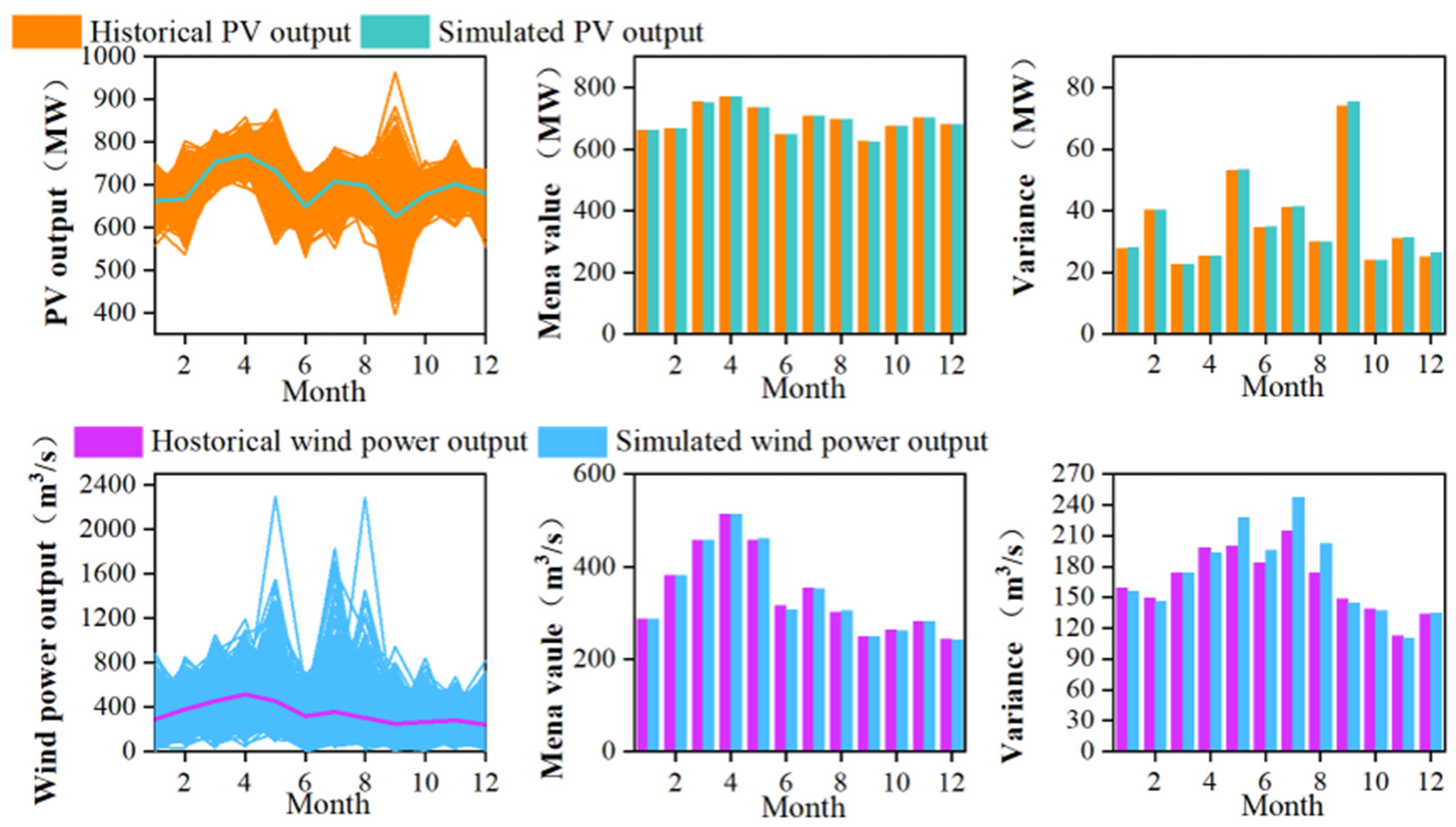
Figure 5.
Technical and economic evaluation indicators under different operation schemes in the historical baseline state.
Figure 5.
Technical and economic evaluation indicators under different operation schemes in the historical baseline state.
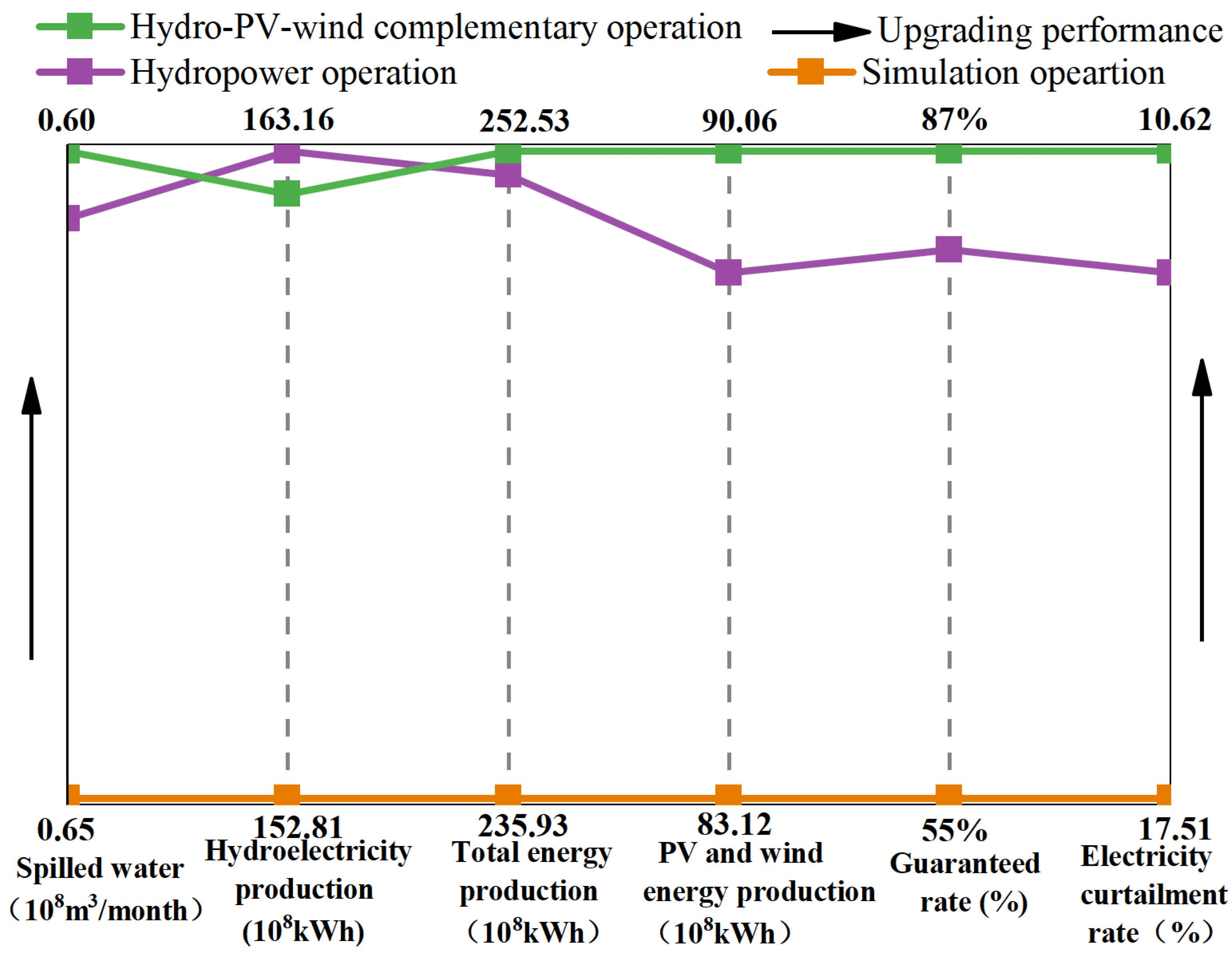
Figure 6.
The HGS’s robustness under different operation schemes.

Figure 7.
Cumulative distribution curves of the technical and economic indicators under uncertain resource scenarios: (a) hydroelectricity production; (b) total energy production; (c) guaranteed rate; (d) spilled water; (e) electricity curtailment rate.
Figure 7.
Cumulative distribution curves of the technical and economic indicators under uncertain resource scenarios: (a) hydroelectricity production; (b) total energy production; (c) guaranteed rate; (d) spilled water; (e) electricity curtailment rate.
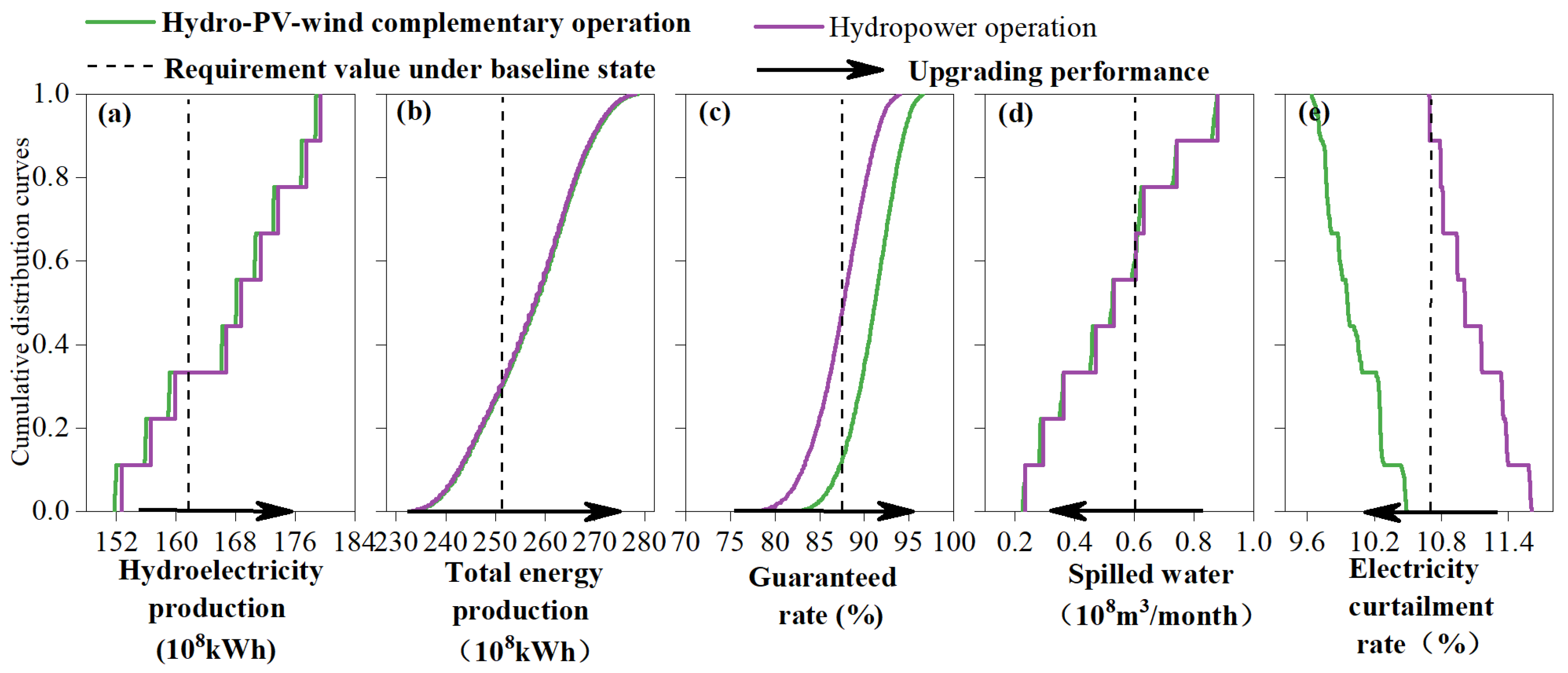
Figure 8.
Comparison of the robustness of the HGS under uncertain scenarios: (a) S1j under PV and inflow uncertainties; (b) S1j under wind power and inflow uncertainties; (c) S1j under PV and wind power uncertainties; (d) S2j under PV and inflow uncertainties; (e) S2j under wind and inflow uncertainties; (f) S2j under PV and wind power uncertainties.

Figure 9.
Robustness indicators under all installed capacity scenarios of PV and wind power plants.

Figure 10.
Robustness indicators under all capacity ratio scenarios of PV and wind power plants.

Table 1.
Parameters of the cascade hydropower plants.
| Parameters | Cihaxia | Banduo | Yangqu | Units |
|---|---|---|---|---|
| Installed capacity | 2600 | 360 | 1200 | MW |
| Dead water level | 2950 | 2757 | 2710 | m |
| Normal water level | 2990 | 2760 | 2715 | m |
| Active storage | 1854 | 2 | 239 | million m3 |
| Upper limit of outflow | 6000 | 6000 | 6000 | m3/s |
| Average hydraulic head | 219.1 | 35.8 | 117.8 | m |
| Lower limit of outflow | 200 | 200 | 200 | m3/s |
| Regulation ability | Seasonal | Daily | Daily | / |
Table 2.
Comparison of mean values of stochastic variables between historical and simulated conditions.
Table 2.
Comparison of mean values of stochastic variables between historical and simulated conditions.
| Uncertainty Scenario | Cihaxia Inflow (m3/s) | Banduo Inflow (m3/s) | Yangqu Inflow (m3/s) | PV Power Output (MW) | Wind Power Output (MW) | |||||
|---|---|---|---|---|---|---|---|---|---|---|
| Historical | Simulated | Historical | Simulated | Historical | Simulated | Historical | Simulated | Historical | Simulated | |
| −10% | 521.6 | 521.3 | 522.2 | 521.3 | 647.2 | 646.3 | 693.8 | 693.1 | 342.0 | 340.9 |
| −9% | 527.4 | 525.2 | 528.0 | 525.2 | 654.4 | 652.6 | 701.5 | 700.8 | 345.8 | 344.7 |
| −8% | 533.2 | 539.1 | 533.8 | 539.1 | 661.6 | 669.2 | 709.2 | 708.5 | 349.6 | 348.4 |
| −7% | 539.0 | 533.5 | 539.6 | 533.5 | 668.8 | 666.2 | 716.9 | 716.2 | 353.4 | 352.2 |
| −6% | 544.8 | 546.1 | 545.4 | 546.1 | 676.0 | 675.4 | 724.6 | 723.9 | 357.2 | 356.0 |
| −5% | 550.6 | 559.9 | 551.2 | 559.9 | 683.2 | 692.6 | 732.3 | 731.6 | 361.0 | 359.8 |
| −4% | 556.4 | 564.9 | 557.0 | 564.9 | 690.3 | 701.7 | 740.0 | 739.3 | 364.8 | 363.6 |
| −3% | 562.2 | 560.3 | 562.8 | 560.3 | 697.5 | 695.4 | 747.7 | 747.0 | 368.6 | 367.4 |
| −2% | 568.0 | 577.2 | 568.6 | 577.2 | 704.7 | 715.3 | 755.4 | 754.7 | 372.4 | 371.2 |
| −1% | 573.8 | 579.3 | 574.4 | 579.3 | 711.9 | 716.3 | 763.1 | 762.4 | 376.2 | 374.9 |
| 0% | 579.6 | 582.7 | 580.2 | 582.7 | 719.1 | 722.4 | 770.8 | 770.1 | 380.0 | 378.7 |
| 1% | 585.4 | 595.6 | 586.0 | 595.6 | 726.3 | 737.9 | 778.5 | 777.8 | 383.8 | 382.5 |
| 2% | 591.1 | 589.3 | 591.8 | 589.3 | 733.5 | 734.2 | 786.3 | 785.5 | 387.6 | 386.3 |
| 3% | 596.9 | 596.5 | 597.6 | 596.5 | 740.7 | 739.2 | 794.0 | 793.2 | 391.4 | 390.1 |
| 4% | 602.7 | 616.3 | 603.4 | 616.3 | 747.9 | 760.7 | 801.7 | 800.9 | 395.2 | 393.9 |
| 5% | 608.5 | 608.3 | 609.2 | 608.3 | 755.1 | 756.1 | 809.4 | 808.6 | 399.0 | 397.7 |
| 6% | 614.3 | 621.9 | 615.0 | 621.9 | 762.3 | 769.0 | 817.1 | 816.3 | 402.8 | 401.5 |
| 7% | 620.1 | 630.9 | 620.8 | 630.9 | 769.4 | 781.9 | 824.8 | 824.0 | 406.6 | 405.2 |
| 8% | 625.9 | 641.7 | 626.6 | 641.7 | 776.6 | 789.9 | 832.5 | 831.7 | 410.4 | 409.0 |
| 9% | 631.7 | 635.5 | 632.4 | 635.5 | 783.8 | 787.6 | 840.2 | 839.4 | 414.2 | 412.8 |
| 10% | 637.5 | 642.8 | 638.2 | 642.8 | 791.0 | 798.7 | 847.9 | 847.1 | 418.0 | 416.6 |
| Maximum deviation | 2.5% | 2.4% | 1.7% | 0.1% | 0.3% | |||||
| Mean deviation | 1.0% | 1.0% | 0.8% | 0.1% | 0.3% | |||||
Table 3.
Comparison of standard deviation values of stochastic variables between historical and simulated conditions.
Table 3.
Comparison of standard deviation values of stochastic variables between historical and simulated conditions.
| Uncertainty Scenario | Cihaxia Inflow (m3/s) | Banduo Inflow (m3/s) | Yangqu Inflow (m3/s) | PV Power Output (MW) | Wind Power Output (MW) | |||||
|---|---|---|---|---|---|---|---|---|---|---|
| Historical | Simulated | Historical | Simulated | Historical | Simulated | Historical | Simulated | Historical | Simulated | |
| −10% | 408.4 | 405.3 | 408.9 | 405.3 | 506.8 | 474.4 | 56.3 | 56.8 | 188.5 | 197.4 |
| −9% | 413.0 | 411.4 | 413.4 | 411.4 | 512.4 | 481.8 | 56.9 | 57.4 | 190.6 | 199.6 |
| −8% | 417.5 | 423.5 | 418.0 | 423.5 | 518.0 | 494.5 | 57.5 | 58.1 | 192.6 | 201.8 |
| −7% | 422.0 | 413.7 | 422.5 | 413.7 | 523.7 | 486.5 | 58.1 | 58.7 | 194.7 | 204.0 |
| −6% | 426.6 | 426.2 | 427.0 | 426.2 | 529.3 | 497.5 | 58.8 | 59.3 | 196.8 | 206.2 |
| −5% | 431.1 | 435.6 | 431.6 | 435.6 | 534.9 | 508.9 | 59.4 | 60.0 | 198.9 | 208.4 |
| −4% | 435.7 | 441.4 | 436.1 | 441.4 | 540.6 | 518.6 | 60.0 | 60.6 | 201.0 | 210.6 |
| −3% | 440.2 | 437.2 | 440.7 | 437.2 | 546.2 | 511.3 | 60.6 | 61.2 | 203.1 | 212.8 |
| −2% | 444.7 | 451.0 | 445.2 | 451.0 | 551.8 | 527.2 | 61.3 | 61.9 | 205.2 | 214.9 |
| −1% | 449.3 | 453.2 | 449.8 | 453.2 | 557.5 | 527.8 | 61.9 | 62.5 | 207.3 | 217.1 |
| 0% | 453.8 | 457.3 | 454.3 | 457.3 | 563.1 | 533.9 | 62.5 | 63.1 | 209.4 | 219.3 |
| 1% | 458.3 | 463.8 | 458.9 | 463.8 | 568.7 | 541.9 | 63.1 | 63.7 | 211.5 | 221.5 |
| 2% | 462.9 | 460.2 | 463.4 | 460.2 | 574.3 | 540.1 | 63.8 | 64.4 | 213.6 | 223.7 |
| 3% | 467.4 | 465.5 | 467.9 | 465.5 | 580.0 | 542.7 | 64.4 | 65.0 | 215.7 | 225.9 |
| 4% | 472.0 | 480.5 | 472.5 | 480.5 | 585.6 | 560.5 | 65.0 | 65.6 | 217.8 | 228.1 |
| 5% | 476.5 | 479.1 | 477.0 | 479.1 | 591.2 | 559.1 | 65.6 | 66.3 | 219.9 | 230.3 |
| 6% | 481.0 | 485.8 | 481.6 | 485.8 | 596.9 | 566.8 | 66.3 | 66.9 | 222.0 | 232.5 |
| 7% | 485.6 | 492.6 | 486.1 | 492.6 | 602.5 | 576.7 | 66.9 | 67.5 | 224.1 | 234.7 |
| 8% | 490.1 | 507.1 | 490.7 | 507.1 | 608.1 | 586.5 | 67.5 | 68.2 | 226.2 | 236.9 |
| 9% | 494.7 | 500.8 | 495.2 | 500.8 | 613.8 | 584.1 | 68.1 | 68.8 | 228.2 | 239.1 |
| 10% | 499.2 | 501.4 | 499.7 | 501.4 | 619.4 | 587.1 | 68.8 | 69.4 | 230.3 | 241.3 |
| Maximum deviation | 3.5% | 3.3% | 7.1% | 1.0% | 4.7% | |||||
| Mean deviation | 1.1% | 1.1% | 5.2% | 1.0% | 4.7% | |||||
Table 4.
Variance-based sensitivity indicators of the HGS’s robustness.
| Sensitive Factors | Rm | S1 | S2 |
|---|---|---|---|
| Installed capacity factor | 0.0672 | 0.1727 | 0.1512 |
| Capacity ratio factor | 0.0025 | 0.0295 | 0.1341 |
Disclaimer/Publisher’s Note: The statements, opinions and data contained in all publications are solely those of the individual author(s) and contributor(s) and not of MDPI and/or the editor(s). MDPI and/or the editor(s) disclaim responsibility for any injury to people or property resulting from any ideas, methods, instructions or products referred to in the content. |
© 2024 by the authors. Licensee MDPI, Basel, Switzerland. This article is an open access article distributed under the terms and conditions of the Creative Commons Attribution (CC BY) license (https://creativecommons.org/licenses/by/4.0/).
Share and Cite
MDPI and ACS Style
Jiang, J.; Ming, B.; Huang, Q.; Bai, Q. Operational Robustness Assessment of the Hydro-Based Hybrid Generation System under Deep Uncertainties. Energies 2024, 17, 1974. https://doi.org/10.3390/en17081974
AMA Style
Jiang J, Ming B, Huang Q, Bai Q. Operational Robustness Assessment of the Hydro-Based Hybrid Generation System under Deep Uncertainties. Energies. 2024; 17(8):1974. https://doi.org/10.3390/en17081974
Chicago/Turabian StyleJiang, Jianhua, Bo Ming, Qiang Huang, and Qingjun Bai. 2024. "Operational Robustness Assessment of the Hydro-Based Hybrid Generation System under Deep Uncertainties" Energies 17, no. 8: 1974. https://doi.org/10.3390/en17081974
Note that from the first issue of 2016, this journal uses article numbers instead of page numbers. See further details here.