

The Study of Multi-Terminal DC Systems in an Offshore Wind Environment: A Focus on Cable Ripple Analysis

1
School of Engineering, University of Warwick, Library Rd., Coventry CV4 7AL, UK
2
Institute for Energy Systems, School of Engineering, University of Edinburgh, Edinburgh EH9 3JL, UK
*
Author to whom correspondence should be addressed.
Energies 2024, 17(8), 1978; https://doi.org/10.3390/en17081978
Submission received: 6 January 2024
/
Revised: 16 April 2024
/
Accepted: 17 April 2024
/
Published: 22 April 2024
(This article belongs to the Collection Women's Research in Wind and Ocean Energy)
Abstract
:This paper studies the THD and AC losses on the DC cables of offshore wind farm-based multi-terminal HVDC systems when they extract and deliver power from and to more than one connection point. In the paper, the study of a full system PLECS + Simulink model with two branches, including a wind resource, a wind turbine, a Permanent Magnet Synchronous Generator (PMSG), a Pulse Width Modulation (PWM) rectifier, a Single Active Bridge (SAB) DC–DC converter, an Input Parallel Output Series (IPOS) DC–DC converter, HVDC cables, and a simplified onshore system, is presented. It focuses on the investigation of the output ripple content of multiple DC–DC converters on DC cables under different wind conditions with different voltage and power ratings. The importance of the study is providing a general understanding of the operation of the innovative offshore wind farm-based DC system, as well as the interaction between different DC–DC converters and their influence on cable ripple content under different situations.
1. Introduction
Wind power is a renewable energy source that has vast potential for further development, as it is perceived as pollution-free and plentiful. However, wind turbines also have negative consequences for the environment (in particular their visual impact). Hence, wind farms are best situated offshore, away from densely populated areas, to capitalize on higher and steadier wind speeds [1,2,3,4]. As is known, most of the electrical energy is consumed in cities, so a way to efficiently transfer such energy over long distances is required.
Some offshore wind farms are close to the shore, while others can be many kilometers offshore. AC submarine transmission cables can be used to connect wind farms located close to the shore, typically less than 50 km in distance, with the onshore power system. For wind farms farther offshore, DC transmission is superior to AC transmission. HVDC submarine transmission cables are usually appropriate when wind farms are built farther than about 50 km from the shore [5,6,7].
This paper focuses on examining a potential multi-terminal MVDC/HVDC system based on offshore wind farms. Notably, it examines a configuration in which the distance between the generating-side wind farm and the onshore power system at the receiving end spans 100 km, as shown in ([8], Figure 1). The typical length of the offshore submarine HVDC cables is between 60 and 200 km, and 100 km is the average value of the typical length [9]. When discussing a multi-terminal DC system, researchers explore various structural configurations and investigate different aspects of the system. Among these configurations, the four-terminal meshed multi-terminal DC (MTDC) system stands out as the most frequently employed [10,11,12,13,14,15]. However, alternative structures such as the four-terminal radial system [16] and the typical structure of a low-voltage MTDC system [17] also receive attention, although none matches the exact structure under consideration in this research.
In studies [10,11,12,16,18], authors primarily focus on DC fault detection and mitigation techniques. Methods include practical low-frequency approaches and utilizing the relationship between the discharged power of DC-link capacitors and the increasing power of the faulted branch. The most effective fault detection strategies are identified to ensure superior performance and validated through simulation.
On the other hand, in [13,19], researchers delve into new methodologies and calculation methods for power flow in MTDC systems under various control modes. Meanwhile, studies [14,15,17,20] concentrate on investigating system stability, encompassing small signal stability and oscillation instability phenomena between different voltage source converters and ensuring stable interoperability among converter systems from different manufacturers. Corresponding problem-solving methods are proposed accordingly.
In the research area of harmonics on HVDC cables, most studies focus on end-to-end HVDC systems, rather than multi-terminal systems. Prior works [21,22] aimed to suppress high-frequency harmonics by employing filters and specific control methods for compensation. In ref. [23], high-order harmonics were significantly reduced through the implementation of a proposed LCL-HVDC converter transformer compared to traditional LCC HVDC systems. In ref. [24], AC filters were the primary focus for harmonics suppression in a simplified single-feed DC system. However, this paper diverges from the focus on harmonics suppression. Instead, it concentrates on examining harmonics under varying wind conditions in an innovative, multi-terminal system to detect potential high-AC ripple content.
Previous studies [25,26,27] treated different sections of the HVDC system, such as transformers, converters, and DC lines, as two-port networks to create efficient models for analyzing harmonic transmission and amplification. They also focused on developing DC-side impedance models and studying DC system harmonic resonance. However, their emphasis on simplified models and research limited to low-frequency ranges in steady-state conditions differs from the focal point of this paper.
The current study proposes a comprehensive model and undertook the prolonged monitoring of AC harmonics while varying wind speeds. Its principal aim is to track the DC voltage and current states, along with their harmonic components, across varying wind speeds experienced by individual turbines, thereby identifying potential issues for the prospective system.
To achieve this, a detailed model encompassing the entire control circuit within each section of the system is constructed for the simulation study. This level of detail is strict for this research, as it allows for the calculation of AC losses on the DC cables through the Fast Fourier Transform (FFT) analysis of the simulation outcomes. A more intricate model ensures greater accuracy in the results. Moreover, the inclusion of the full control circuit is essential because the power transfer characteristics are entirely influenced by wind conditions.
The contributions of this paper can be summarized as follows:
- The total harmonic distortion of terminal voltages was analyzed across different wind conditions and system configurations, consistently maintaining voltages below 2%. This performance surpasses expectations, especially notable in multi-connected cable terminals in which a high current ripple and superimposed currents might induce significant voltage variations;
- Research into cable AC losses examined variations across diverse wind conditions and system configurations, distinguishing their characteristics in both multi-connected submarine cables and those in 100 km;
- The system’s dynamic performance under extreme wind conditions reveals its resilience, notably in swiftly recovering from brief deviations below or above the cut-in and cut-out wind speeds. Such resilience is attributed to the infrequent occurrence of unexpected wind fluctuations, which typically affect only a few turbines within large wind farm systems for short periods;
- The performance of various ISIPOS converter structures is compared, and corresponding application environments are suggested.
In this study, the simulation results of a two branch, multi-terminal system under different wind conditions are presented with a concentration on the cable voltage ripple, current ripple, and AC losses.
2. Overview of the Simulation Model
2.1. Circuit Diagram and Specification of the Simulation Model
Figure 1 shows a two-branch, multi-terminal DC system, which is the circuit of the simulation model in this study. This figure displays a more detailed circuit diagram of the generating side in ([8], Figure 1), and the system specification is described as follows:
Wind Model:
This study focuses on wind power as the sole energy input source. Irrespective of wind direction, the wind model is characterized by various parameters, including the natural wind speed (SWt), the fundamental wind speed (SWb), the gust wind speed (SWg), the ramp wind speed (SWr), and the noise wind speed (SWn), as shown in Equation (1). An illustrative example of the natural wind model is provided in Figure A3 [28].
Wind Turbine:
The wind turbine simulation module was constructed based on the specifications of the 5 MW AD5135 turbine, detailed in Table 1. The turbine’s output power is a function of its power coefficient (Cp) and mechanical rotation speed (m), as expressed in Equation (2). This equation factors in parameters including the air density (), blade length (R), wind turbine tip speed ratio (), pitch angle (), wind speed (Vw), rated wind speed (Vrated), cut-in wind speed (Vcut-in), and cut-out wind speed (Vcut-out). Within the maximum power point tracking (MPPT) region, Equation (3) describes the relationship between wind velocity and output power.
The control circuit design of the wind turbine is based on Equations (2) and (3). Output power is absent when the wind speed falls below the cut-in value. Within the MPPT region (between the cut-in and rated speeds), the control system optimizes the power output by adjusting the rotor speed or pitch angle. Within the rated speed and cut-out speed range, the turbine operates at a constant full-power state, delivering 5 MW. No output power is generated when the wind speed exceeds the cut-out value.
Permanent Magnetic Synchronous Generator (PMSG) and Pulse Width Modulation (PWM) Rectifier:
The Permanent Magnet Synchronous Machine (PMSM) is an electrical device distinguished by its rotor, which is magnetized via permanent magnets, eliminating the need for an additional DC excitation circuit. While the Double-Fed Induction Generator (DFIG) remains prevalent in offshore wind farms, the Permanent Magnet Synchronous Generator (PMSG) has gained traction as an appealing alternative for wind turbine applications. The flux linkage equation, stator voltage equation, and power relationship of PMSG can be seen in Equation (4).
In this study, the authors employed 5 MW PMSGs with a frequency of 55 Hz and a power factor of 0.9, featuring a rated line voltage of 2.86 kV and a rated line current of 1.12 kA [29]. The selection of the machine’s power rating is contingent upon the wind turbine’s capacity, with its actual operational line voltage determined by the connected PWM rectifier. Based on Equation (5), given an output voltage of 5 kV DC for the PWM rectifier, the input voltage (Vline_rms) of the PWM rectifier is computed as 2.6 kV, aligning with the output line voltage of the PMSG, under the assumption of a modulation index (m) of 0.85. It is important to note that the modulation index will vary, depending on the total power transferred, with 0.85 chosen as a standard value for design purposes [30]. Further specifications of the PWM rectifier are detailed in Table 2.
5 MW DC–DC converter:
A 5 MW DC–DC converter, operating within a voltage range of 5 kV to 50 kV, is integrated into the offshore wind farm’s multi-terminal DC system. Its power rating corresponds to that of the wind turbine, 5 MW AD5135. Both the input and output voltage selections were informed by prior research on high-power DC–DC converters for offshore wind DC systems [31]. Detailed converter parameters are listed in Table 3.
Input Series Input Parallel Output Series (ISIPOS) DC–DC Converter:
In the context of ([8], Figure 1), the Input Series Input Parallel Output Series (ISIPOS) converter plays an important role in gathering power from the entire wind farm and stepping up the voltage subsequent to the multi-terminal connection. To streamline the simulation processes, the 200∼1000 MW ISIPOS converter was downsized to a 30 MW Input Parallel Output Series (IPOS) converter, as depicted in Figure 1. Increasing the number of series-connected IPOS blocks merely reduces the I/O voltage and power of each identical block without significantly altering simulation outcomes or impacting the overall performance of the high-power, high-voltage ISIPOS converter within the system. The detailed specifications of the ISIPOS Converter are outlined in Table 4.
The detailed structure and circuit diagram of the Input Parallel Output Series (IPOS) DC–DC converter were provided in ([8], Figure 4), resulting in three different unidirectional constructions within the simulation model [32]; this paper solely presents the system performance with the Identical Three-Phase Bridge IPOS Converter in ([8], Figure 4b) and the Identical SAB IPOS Converter in ([8], Figure 4c), as the performance of the system with the SAB + Three-Phase Bridge IPOS Converter in ([8], Figure 4a) was expected to fall between them. All parameter labels in the simulation results were derived from Figure 1, with a comprehensive study conducted on the impact of the cable ripple content and AC losses from various perspectives.
MVDC/HVDC Undersea Cables:
Long submarine cables were employed to transfer power from the offshore wind farm to the onshore power system post-ISIPOS converter. A model, as shown in Figure 2, was used to represent the equivalent circuit of these cables, facilitating the analysis of AC ripple content via an FFT frequency spectrum. Cable parameters are outlined in Table 5 and Table 6.
2.2. Circular Wind Farm Structure
Figure 3 displays a concept graph of a circular wind farm. This type of structure has been studied for a few years but has not yet been built in real life. The circular wind farm can be regarded as a composition of concentric circles, and turbines are installed on the circumferences of these rings. X, which obeys the 5D principle, in Figure 3 represents the distance between two adjacent turbines at the same circumference. The radius difference between two adjacent concentric circles should be set to at least ten times X to eliminate the influence between different circles. This is why the length of the cable through which I5 is flowing is set to 6 km in Figure 1.
Compared with the array structure, one significant advantage of the circular wind farm is that the wind speed, or power, received at turbines constructed on the same ring is the same regardless of the wind direction. In other words, the wake effect and turbulence are eliminated dramatically, and a more straightforward control method can be applied. As for the disadvantages, a circular-structure wind farm needs more space, and longer submarine cables are necessary to connect the turbines at different circumferences. Overall, the circular wind farm structure may attract higher commercial interest compared to the traditional array structure, mainly due to its higher wind power utilization ability, and it was used in this study [29].
2.3. Selection of the Phase Angle of Different DC–DC Converters
As mentioned in [8], it can be challenging to synchronize the IGBT switching of all the multi-connected 5 MW DC–DC converters due to the long distance between them, and the extreme condition study method was applied in the simulation model, while the average value of the results obtained from the following two conditions can be regarded as the normal performance of the system.
- All the switches of these six multi-connected 5 MW converters are controlled via the same signal;
- There are 60-degree phase shifts between the switches’ control signals of these 5 MW, multi-connected SAB converters.
3. Simulation Study of the System under Different Wind Conditions
In this simulation work, the system operated under different natural wind conditions, including gust and ramp wind, which means that results from a much longer simulation time needed to be monitored compared to the switching periods of the power electronic devices in the system. The steady or constant wind speed received at each turbine was set to around 10.3 m/s, which is the 10-year average wind speed of the area where the Hywind Scotland Pilot Park project was built [8,33]. The transient states are involved since the power derived from the wind is not constant, and the simulation results of the system with both Identical Three-Phase IPOS and Identical SAB IPOS structures are presented and compared.
The speed change of all the natural winds in this study started after 7 s and returned back to the base wind speed before 15 s; all the results presented under the natural wind conditions occurred within this time period.
Based on the study in [8], the output capacitors of all the 5 MW multi-connected DC–DC converters were set to 40 F, and the input capacitors of the Identical Three-Phase IPOS converter were set to 0.4 F. The input capacitors of the Identical SAB IPOS converter were selected as 4 F.
3.1. Simulation Results of the System with Identical Three-Phase and Identical SAB IPOS Converter Structures under Wind Condition 1
3.1.1. Wind Condition 1
When referring to Appendix A, situation 1, and the wind model study in [28], the wind speed received by each turbine in this situation can be seen in Figure 4. Notably, turbines WT1 and WT2 encountered gust and ramp winds, while the remaining turbines operated under steady wind conditions.
In Figure 4, WT1 to WT6 are wind turbines 1 to 6 in Figure 1; the wind noise was not included for better clarity. A graph showing an example of natural wind with noise can be seen in Figure A3 in Appendix B.
3.1.2. Vdc1 and Idc1 When the Identical SAB IPOS Structure Is Applied in the System and There Is No Phase Difference between 5 MW SAB DC–DC Converters
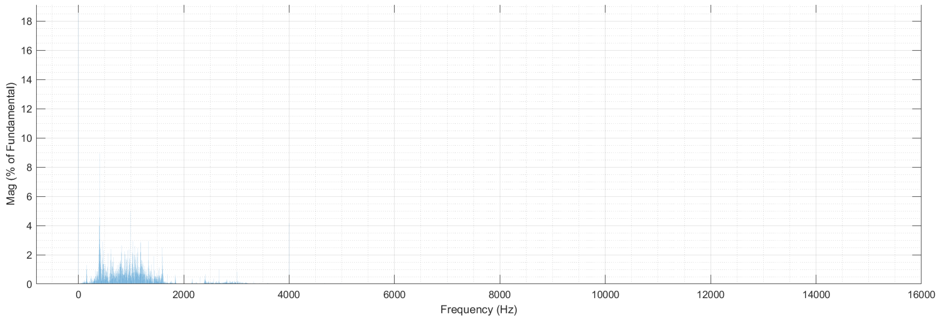
In wind condition 1, wind turbine 1 experienced an increase in wind speed, resulting in observable waveforms for Vdc1 and Idc1, as depicted in Figure 5. During time period A, transitioning from the Maximum Power Point Tracking (MPPT) region to the constant full-power region, or during time period B, when returning to the MPPT region, the waveform exhibited lower ripple content or total harmonic distortion compared to when the power was constant. In this study, the FFT analysis focused on the constant full-power region to discern the harmonic properties of the waveform. Consistency was maintained throughout the paper by utilizing the same period for the FFT analysis to ensure unbiased comparisons. Figure 6 and Figure 7 illustrate the harmonic voltage and current spectrum for Vdc1 and Idc1 in Figure 5. It is important to note that the baseline value of the harmonic spectrum for Idc1 is defined as 63 A, rather than the actual DC components, for normalization purposes.
Figure 5.
Vdc1 and Idc1 with identical SAB IPOS structure.

Figure 6.
Harmonic spectrum for Vdc1.
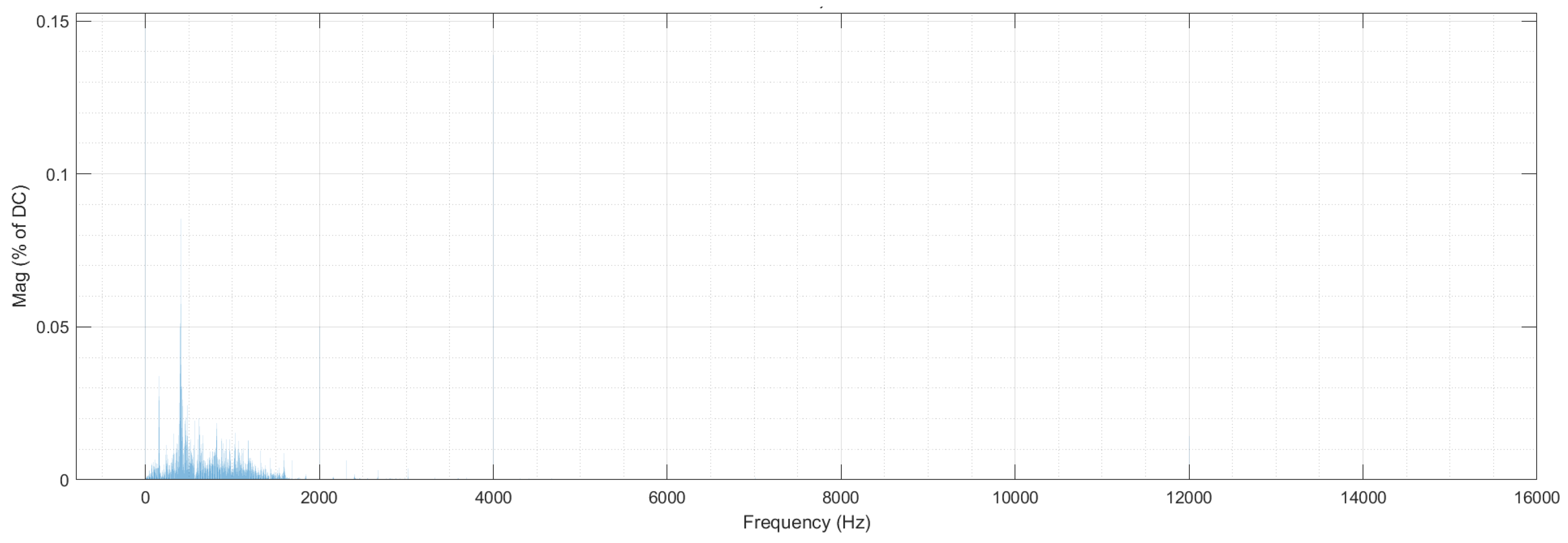
Figure 7.
Harmonic spectrum for Idc1.
3.1.3. Waveforms of Terminal Voltages and Cable Currents Based on the Average Values under Wind Condition 1
As can be seen from Figure 5, when comparing the waveforms of all the terminal voltages or cable currents in one figure, massive overlapping of the waveforms occurs, and the graphs can become meaningless. One way to plot sensible graphs is by drawing the waveforms based on the average values during a specific period, as shown in Figure 8, Figure 9 and Figure 10, when the specific period is set to be 0.05 s.
As for the waveforms of Vo and Io, both their average value graphs and original waveforms are shown in Figure 11 and Figure 12.
Figure 8.
Graphs of average voltage at the terminals of all 0.6-km/6-km cables.
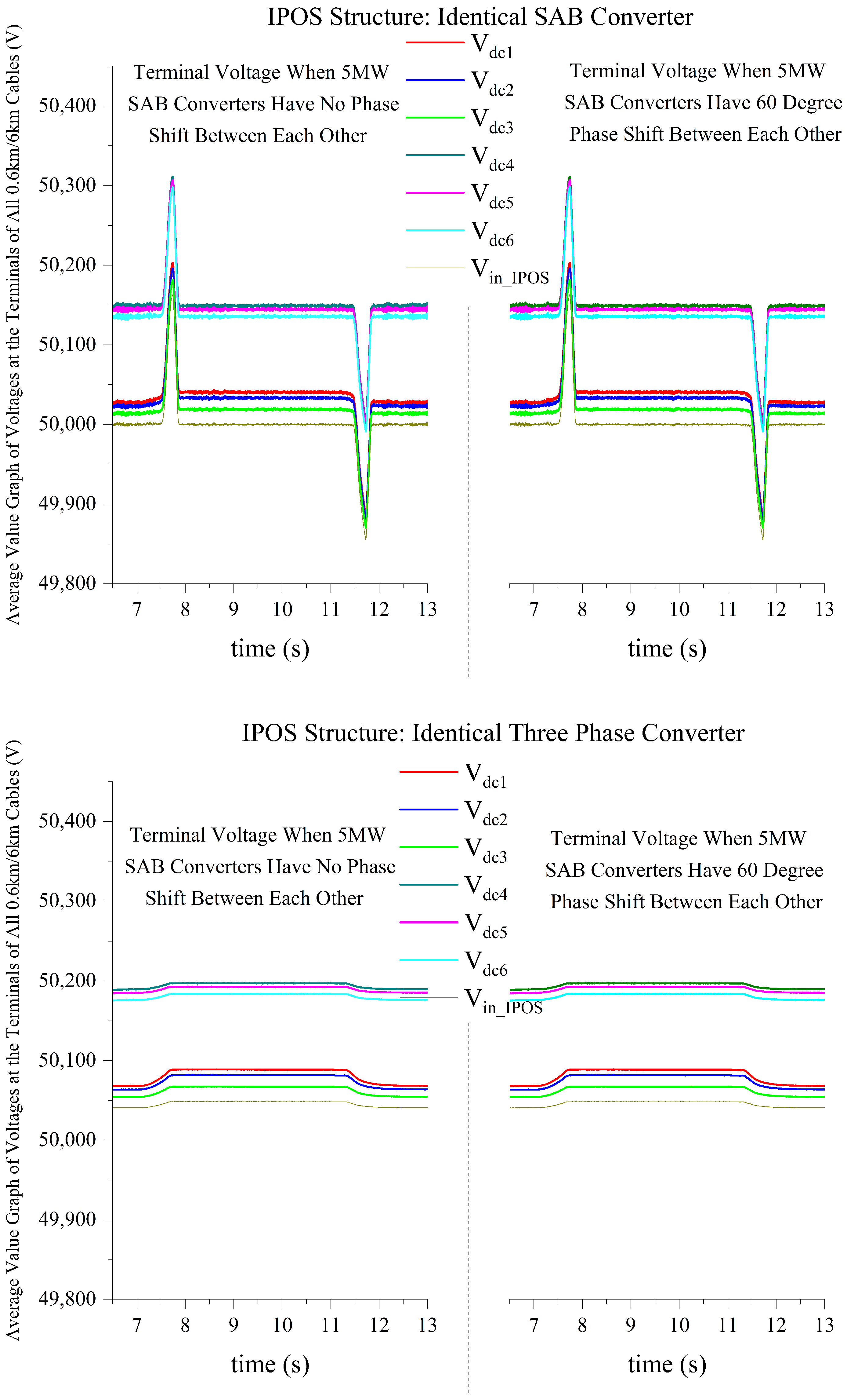
Figure 9.
Graphs of average output currents for 5 MW SAB converters.

Figure 10.
Graphs of average currents on the multi-connected cables.

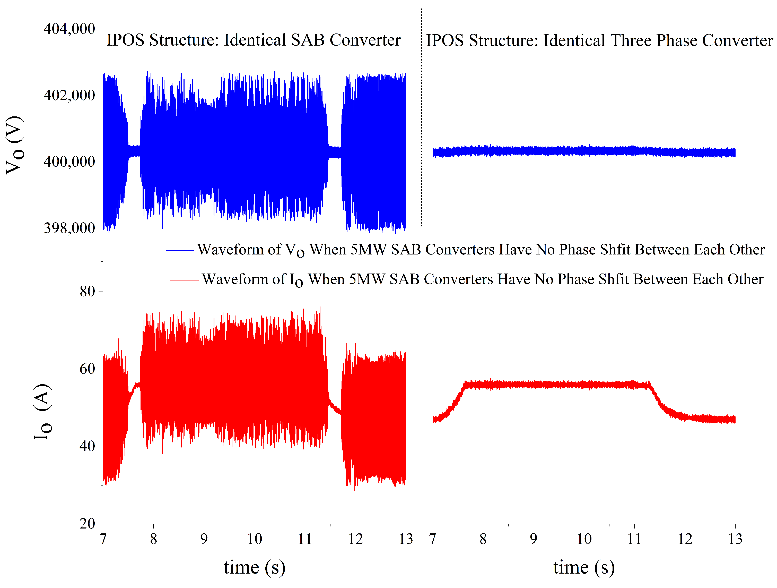
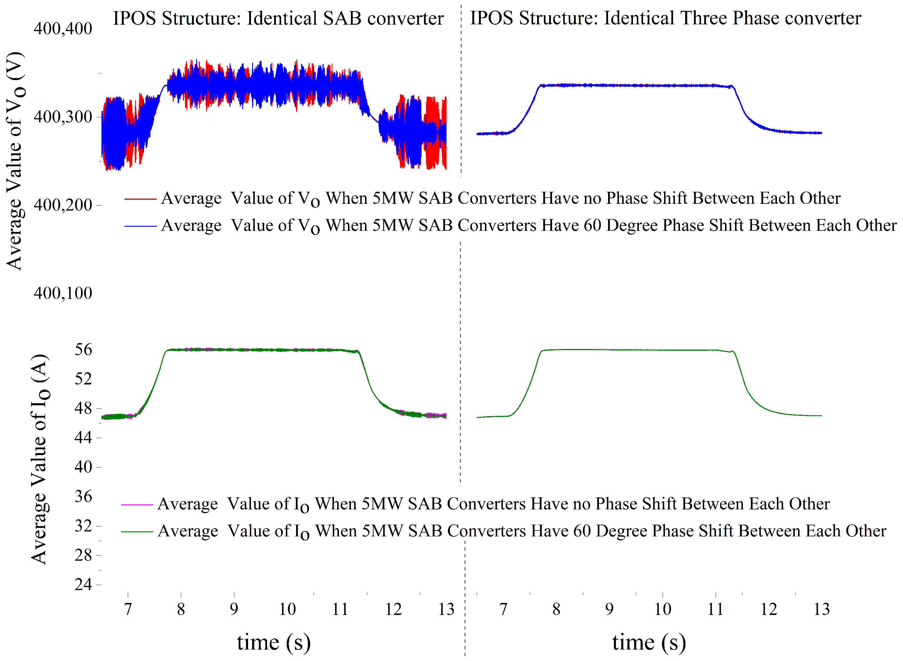
Figure 11.
Average value graphs of Vo and Io.

Figure 12.
Waveforms of Vo and Io.
As per Figure 8, Figure 9, Figure 10, Figure 11 and Figure 12, some observations are presented as follows:
- In Figure 8, for a system with the Identical SAB IPOS structure, the DC value of Vin_IPOS is controlled well at 50 kV, while that of the system with the Identical Three-Phase IPOS structure is mostly dependent on the DC voltage value at the receiving end of the system and the current flow through the transmission cables. It can be noticed that the value of Vin_IPOS in the system with the Identical Three-Phase IPOS structure increases with increasing wind power; this is due to an increase in the DC component/average value of Io when more power is fed into the system, leading to a higher voltage drop on the 100-km transmission cables;
- The current superposition along the multi-connected cables towards the receiving end of the system is shown in Figure 9 and Figure 10. These cable currents result in a voltage drop on the multi-connected cables, which can be seen in Figure 8. It should be noted that the 6-km cable with I5 flowing through it undergoes a higher voltage drop in the system, as its equivalent resistance is ten times higher than that of the 0.6-km cables;
- Figure 13 shows the waveform of Vdc1 and Idc1 when the Identical Three-Phase IPOS structure is used in the system. When comparing Figure 5 with Figure 13, it is clear that, during the time when the captured wind power is increasing or decreasing, the terminal voltages and currents have lower ripple content but a higher or lower DC value in the system with the closed loop-controlled SAB IPOS structure, which also explains the ”average voltage spike” in Figure 8. The appearance of the reduced ripple content with the controllable Identical SAB IPOS converter is because of the variation in the duty ratio of the IPOS converter, which can lead to phase changes in the ripple content;
- As expected, in Figure 11 and Figure 12, the average power transferred to the onshore power system is similar in systems with different IPOS converter structures under the same wind condition. Nonetheless, the advantage of reduced cable ripple content in the system employing the Identical Three-Phase IPOS structure is distinctly evident. A more detailed FFT analysis of the system under this wind condition is presented in Section 3.4.
Overall, if the voltage at the receiving end of the system can be controlled so that it maintains a relatively constant value, or the onshore power system is robust enough, a controllable IPOS structure is not a necessary choice if Io in the 100-km cables is not large enough to cause more than a ±5% [31,34,35] voltage difference with respect to the rated value.
3.1.4. FFT Analysis of DC Cable Voltage and Current AC Ripples
To enhance the understanding of submarine cable ripple content or cable AC losses, a Fast Fourier Transform (FFT) algorithm for waveform analysis was employed. This method effectively dissects complex ripples into sinusoidal waves of varying frequencies, enabling the individual scrutiny of each wave’s impact. In this study, since the fundamental voltage components are solely DC, the total harmonic distortion (THD) of the DC voltage can be seen in Equation (6). Here, Vdc represents the DC fundamental component, while Vn signifies the peak value of the nth harmonic voltage, derived from FFT analysis of the voltage waveform.
The FFT analysis results under wind condition 1 with the Identical SAB IPOS converter structure are shown in Table A1 of Appendix C. This is an example of the percentage of the harmonic wave relative to the base value at the dominant frequency, and the THD results in other situations is shown in Table 7 and Table 8 of Section 3.4 directly, focusing on the period of the FFT region in Figure 5.
The definition of Total Relative Losses was stated in [8], and the relationship between the real losses and the Relative Losses can be seen in Equation (7).
where PRL is the real AC losses caused by harmonics on cables, P4Base is the real losses caused by 4 kHz harmonic with a 1-A amplitude on a 1-km specific cable applied in the system, Ibase is the base value selected when calculating the Relative AC Losses, Lcable is the length of the submarine cable, 2 is an integer that indicates the onward and returned submarine cables, and TRL is the Total Relative AC Losses defined in [8] and caused by harmonics at different frequencies.
3.2. Simulation Results of the System with Identical Three-Phase and Identical SAB IPOS Converter Structures under Wind Condition 2
3.2.1. Wind Condition 2
According to Appendix A situation 2 and the wind model study in [28], the wind speed received at each turbine in this situation can be seen in Figure 14, in which gust and ramp wind happen on WT1, WT4, and WT5, and all other turbines are working under a steady wind speed.
3.2.2. Simulation Results of Vdc1 and Idc1 under Wind Condition 2
Figure 15 shows the waveforms of Vdc1 and Idc1 of the system under natural wind condition 2 with the Identical SAB and Identical Three-Phase IPOS converter structures. The black ellipses in the figure indicate the periods of the signal with relatively high THD or ripple content. It can be seen in the system with the Identical SAB IPOS converter structure that both the terminal voltages and cable currents have a higher ripple content when turbines 1, 4, and 5 are all working with increasing wind speed and are still in the MPPT region. This is not shown in the system with the Identical Three-Phase IPOS converter structure, which has IPOS converters with a fixed duty ratio.
In this part, the FFT analyses concern the periods of the waveforms with a relatively high ripple content in order to identify any significant ripple content or losses caused by the interaction of different turbines working under an asynchronous dynamic wind speed. The FFT analysis results can be seen in Table 7 and Table 8 in Section 3.4.
3.3. Simulation Results of the System with Identical Three-Phase and Identical SAB IPOS Converter Structures under Wind Condition 3
3.3.1. Wind Condition 3
According to Appendix A situation 3 and the wind model study in [28], the wind speed received at each turbine in this situation can be seen in Figure 16, in which gust and ramp wind are experienced at WT2, WT3, WT4, and WT5, and all the other turbines are working under a steady wind speed.
3.3.2. Simulation Results of Vdc1 and Idc1 under Wind Condition 3
Figure 17 shows the waveforms of Vdc1 and Idc1 of the system under wind condition 3 with Identical SAB and Identical Three-Phase IPOS converter structures. It can be seen that, when a few turbines in the system are working under asynchronous but overlapped unstable wind conditions, the reaction of the closed-loop controlled SAB IPOS converter is reflected clearly on the voltage and current waveforms, while the waveforms in the system with the open loop controlled IPOS structure are consistent from beginning to end. As stated before, all the FFT analyses were taken for the periods of the waveforms with a relatively high THD or ripple content in the black ellipses, and the results can be seen in Table 7 and Table 8 in Section 3.4.
3.4. Comparison of the Simulation Results of the Double Branch System under Wind Condition 1–3
The FFT analysis of the double branch system based on wind condition 1–3 can be summarized in Table 7 and Table 8, where the following applies:
TP: System with Identical Three-Phase IPOS converter structure.
SAB: System with Identical Single Active Bridge IPOS converter structure.
WC 1: System working under wind condition 1.
WC 2: System working under wind condition 2.
WC 3: System working under wind condition 3.
TRL-MS: Total Relative AC Losses on the multi-connected cables.
100 kmTL: Relative AC Losses on the 100-km submarine cables.
100 kmTL′: The referred value of the Relative AC Losses from the 100-km cables to the multi-section cables.
Io (DC): The DC component of the 100-km cable current Io.
Ibase: The base value of 47 A for the 100-km cable current.
The relationship between the 100 kmTL and 100 can be seen in Appendix D.
After combining Table 7 and Table 8, the overall performance of the system under different natural wind conditions can be concluded as follows:
- The THD of all terminal voltages is well below 2% even though the FFT analyses were based on the region with a relatively high ripple.
- The Total Relative AC Losses on multi-section cables increased with the increase in the total power transferred; however, the efficiency relative to the AC losses on the multi-section cables is independent of the total power transferred.
- The Total Relative AC Losses on the 100-km cable did not follow the variation in the total power transferred in the system but remained approximately constant. Therefore, the efficiency of the system can be enhanced if more power is extracted from the wind.
- Referring to Equation (A3) in Appendix D, the referred value of the Total Relative AC Losses for the 100-km cable is listed in Table 8 as 100 . It is shown that the 100-km cable’s relative AC losses in the system with the Identical SAB IPOS converter structure were about twenty times those of the Identical Three-Phase IPOS converter or about 50 kW higher in the system with six turbines. However, for a system with an Identical SAB IPOS converter structure, the main losses occur in the 100-km submarine cables, and they are much greater than the losses for the multi-connected cables. As the losses for the 100-km cable do not increase with an increasing power transfer, the superiority of the system with the Identical Three-Phase IPOS converter structure will reduce with an increase in the number of turbines, branches, or transferred power, but it will remain superior.
In summary, the advantages of the system with the open loop controlled Identical Three-Phase IPOS converter structure were demonstrated under these natural wind conditions, even with a smaller filter capacitor value, despite the situation when the receiving end voltage may fluctuate. Moreover, when combining Figure 5, Figure 12, Figure 13, Figure 15 and Figure 17, Table 7 and Table 8, no significant high ripple content or losses are brought into the system, although the variable wind speed experienced at some turbines during a short time period can vary the THD or ripple content of the voltage or current waveforms. The performance of the system is favorable under different wind conditions without a cut-off, and the operation of the system with a single cut-off wind turbine is illustrated in the next section.
3.5. Simulation Results of the System with Identical Three-Phase and Identical SAB IPOS Converter Structures under Wind Condition 4: Cut-Off
3.5.1. Wind Condition 4
According to Appendix A situation 4 and the wind model study in [28], the wind speed at each turbine in this situation can be seen in Figure 18. Based on Figure 18, the natural wind speed on wind turbine 1 reaches the cut-off value of 25 m/s at around 9 s and decreases back down below 25 m/s at around 10 s, while all other turbines are assumed to be working under a steady wind speed.
3.5.2. Simulation Results of All Terminal Voltages and Cable Currents under Wind Condition 4 with Cut-Off
Figure 19, Figure 20 and Figure 21 show the waveforms of the terminal voltages and cable currents of the system between 9 s and 11 s, which includes the entire cut-off period. An FFT analysis is not provided in this section, as there was no significant ripple content or losses present during the cut-off period, and the performance of the system was analyzed based on the waveform graphs. All the figures were obtained when all the 5 MW SAB converters had no phase shift between each other.
When the wind speed blowing at Wind turbine 1 increased to the cut-off wind speed, the power generated via turbine 1 decreased at a sharp rate, and the value of Idc1 was reduced, together with the reduction in the generated power. It was noticed that the value of Idc1 in both cases in Figure 20 can become negative, as part of the Idc2 will flow back to the 5 MW DC–DC converter connected after the PMSG & PWM Rectifier1 in Figure 1, charging its output filter capacitor. All the multi-connected cable currents were added together, and after the transformation of the IPOS converter, Io in Figure 21 indicates the total power generated. It was noticed that, for the system with an Identical SAB IPOS converter structure, the THD, or ripple content, of Io decreased to a relatively small value during the middle time slot in Figure 21. This was mainly because of the variation in the duty ratio of the Identical SAB IPOS converter during the transient state, and this phenomenon cannot be regarded as the property of the system; rather, it depends on the physical parameters when building the system in the real world.
The decrease in current Io causes a reduction in the voltage drop for the 100-km submarine cables, as well as Vo; however, compared with 400 kV, the variation in Vo is negligible, and Vo can almost be regarded as constant. The control system will not react significantly to this voltage drop.
In Figure 19, all terminal voltages decrease slightly during the cut-off because of the current in the multi-section cables and in the IPOS converter itself.
In summary, in this type of multi-connected system, a single wind turbine (or a few wind turbines in a bigger system) that cuts out from the system for a short time period will not cause any significant problems in the system, and the time needed for the recovery is much shorter than that required to start up a turbine until it reaches a steady state, although the recovery time in the real world can be longer than that in the simulation.
4. Conclusions
This paper primarily evaluated the voltage ripple content and AC losses of submarine cables in a system, as well as the operation ability of the system, under different wind conditions, in order to identify any significant influences that can be caused due to a variation in wind speed. According to the study of the system under different wind conditions, the following points can be concluded:
- The total harmonic distortion of all the terminal voltages can be limited to well below 2% in any type of wind condition, with different IPOS converter structures when proper filter capacitors are applied in the system. This result is much better than the expectation, especially when looking at the terminal voltages at the multi-connected cables of the system, as relatively high current ripple content and the superposition of the current may cause high voltage ripple content.
- At all times, a higher power transfer amounts to little more than higher losses in the system. However, in this study, it was found that the AC losses for the 100-km submarine cable did not increase with an increase in the total power transferred, and they remained stable under all conditions.
- The AC losses for the multi-connected submarine cables were in direct proportion to the total power transferred, which is the normal situation.
- Gust winds and interactions between the wind turbines in a wind farm do not cause significant ripple content or AC losses in cables. Before this study, it was opined that the variation in wind speed may produce higher cable ripple content. However, the results lead to the opposite conclusion, and hence, variable wind does not need to be included in the study of the ripple content of cables in future work. The variation in wind speed and the interaction between wind turbines can still influence the power that can be absorbed by the turbines, and it must be considered when looking at the power transfer ability of the system.
- The system has relatively good recoverability when the wind speed is below the cut-in speed or above the cut-out speed for a short period of time, based on the fact that unexpected high or low wind occurs only occasionally and will only impact a few turbines at a large wind farm system during a short period. During the cut-off time, no significant high ripple content or AC losses occur, ruling out the concern before the study.
- Compared with the closed loop controlled SAB IPOS converter structure, the open loop duty ratio controlled Three-Phase IPOS converter can help reduce the value and size of passive filters, leading to the lowest cable ripple content and AC losses, and it can have a high power carrying ability. Against this background, if the onshore power system at the receiving end is robust enough or can always provide a relatively constant voltage value, the Identical Three-Phase ISIPOS converter should be used in the system. However, in a system whose receiving end is likely to fluctuate, the closed loop input voltage-controlled SAB converter should be applied in the IPOS converter structure of the system.
Overall, this type of novel offshore wind farm-based, multi-connected DC system is reliable and can be adequately operated without any significant technical difficulty. The cable ripple content and AC losses are limited under different wind conditions even when a realistically sized filter is implemented in the system.
Author Contributions
Conceptualization, X.R. and D.E.M.; methodology, X.R.; software, X.R.; validation, X.R., J.K.H.S. and D.E.M.; formal analysis, X.R. and D.E.M.; investigation, X.R., J.K.H.S. and D.E.M.; resources, X.R. and P.M.; data curation, X.R.; writing—original draft preparation, X.R.; writing—review and editing, X.R., J.K.H.S. and D.E.M.; visualization, X.R., J.K.H.S. and D.E.M.; supervision, J.K.H.S., D.E.M. and P.M.; project administration, D.E.M. All authors have read and agreed to the published version of the manuscript.
Funding
This research received no external funding.
Data Availability Statement
The original contributions presented in the study are included in the article, further inquiries can be directed to the corresponding authors.
Conflicts of Interest
The authors declare no conflicts of interest.
Appendix A. Possible Wind Conditions at Each Wind Turbine under Different Natural Wind Situations
Before the study of the double branch system with a circular wind farm structure under natural wind/gust situations, some possible wind conditions at each wind turbine should be identified first.
Case 1 (Figure A1):
Figure A1.
Schematic diagram of wind direction in case 1.
The natural wind direction in case 1 is perpendicular to the connecting line of two adjacent wind turbines linked on the same branch, and all the black dots in Figure A1 represent the wind turbines. The value of X1 in figure can be calculated as follows:
if there are ten wind turbines connected with each branch.
Case 2 (Figure A2):
Figure A2.
Schematic diagram of wind direction in case 2.
The natural wind direction in case 2 is perpendicular to the tangent line, which passes through one of the turbines, of the circle. The value of X2 in Figure A2 can be calculated as follows:
if there are ten wind turbines connected with each branch.
In this study, the average speed of the combination of gust, ramp, and fundamental wind is about 18 m/s, while the period of the blustery condition is always less than 10 s [28]. The distance at which the bluster can drift is about 18 × 10 = 180 m. Both the values of X1 and X2 are longer than 180 m, which means the maximum number of turbines that can be influenced by a sudden bluster on one branch of the system is 2. Using the discussion above, four different situations could be put into the simulation:
- In Figure 1, turbine 1 and turbine 2 are affected by the bluster simultaneously, while all other turbines are working under a steady free stream;
- In Figure 1, turbine 4 and turbine 5 are affected by the bluster simultaneously, and turbine 1 is moved by the bluster with a few seconds’ delay, while all the other turbines are working under a steady free stream;
- In Figure 1, turbine 2, turbine 3, turbine 4, and turbine 5 are influenced by an asynchronous bluster, while all the other turbines are working under a steady free stream;
- In Figure 1, turbine 1 is affected by the bluster, which surpasses the cut-out speed, while all the other turbines are working under a steady free stream.
Appendix B. Natural Wind Example
Figure A3 shows an example of the natural wind model applied widely in this study. The natural wind speed is composed of the fundamental wind speed, gust wind speed, ramp wind speed, and noise wind speed [28].
Figure A3.
Natural wind profile.
In the simulation study, a rate limiter with a reasonably high slew rate was added to the natural wind model to avoid a sudden change in the wind speed with an infinite rate value. A step change in the wind speed is not only unrealistic but also causes iteration exceeding/convergence problems in the simulation model [36].
Appendix C. FFT Analysis under WC 1 with Identical SAB IPOS Converter Structure
Table A1 presents the percentage of dominated harmonic frequency in relation to the DC components. It is important to note that only data pertaining to dominated frequencies are incorporated in this table. However, for the calculation of THD or Total Relative losses in Table 7 and Table 8, a significantly broader frequency spectrum range (2 Hz to 20 kHz with a 2-Hz interval) was utilized to enhance the results’ accuracy.

Table A1.
Percentage of harmonic wave relative to the base value at the dominant frequency in a system with Identical SAB IPOS Converter structure when the system is working under WC 1.
Table A1.
Percentage of harmonic wave relative to the base value at the dominant frequency in a system with Identical SAB IPOS Converter structure when the system is working under WC 1.
| Converter Type: Balanced (Identical SAB) IPOS Converter Base Value: Vdc = 50 kV Swb = 10.31 m/s Power = 3.2 MW Idc = 63 A Non: 5 MW SAB No Phase Shift 60: 5 MW SAB 60 degree Phase Shift 5 MW SAB Output Capacitor Value: 40 F 30 MW IPOS Converter Input Capacitor Value: 4 F | ||||||||||
|---|---|---|---|---|---|---|---|---|---|---|
| Frequency | 4 kHz | 8 kHz | 12 kHz | 16 kHz | ||||||
| HP * % | Non | 60 | Non | 60 | Non | 60 | Non | 60 | ||
| V/I | ||||||||||
| Vdc1 | 0.14 | 0.13 | 0.03 | 0.03 | 0.01 | 0.01 | 0.01 | 0.01 | ||
| Vdc2 | 0.18 | 0.18 | 0.04 | 0.04 | 0.01 | 0.01 | 0.01 | 0.01 | ||
| Vdc3 | 0.16 | 0.12 | 0.03 | 0.03 | 0.01 | 0.01 | 0.01 | 0.01 | ||
| Vdc4 | 0.13 | 0.14 | 0.03 | 0.03 | 0.01 | 0.01 | 0.01 | 0.01 | ||
| Vdc5 | 0.13 | 0.16 | 0.03 | 0.03 | 0.01 | 0.01 | 0.01 | 0.01 | ||
| Vdc6 | 0.13 | 0.14 | 0.03 | 0.03 | 0.01 | 0.01 | 0.01 | 0.01 | ||
| Vin_IPOS | 0.2 | 0.15 | 0.01 | 0.01 | 0.4 | 0.4 | 0 | 0.01 | ||
| Idc1 | 4.2 | 15.5 | 0.2 | 2.69 | 0.05 | 0.83 | 0.02 | 0.29 | ||
| I2 | 21.26 | 6.7 | 2.6 | 0.63 | 0.8 | 0.01 | 0.13 | 0.15 | ||
| I3 | 30.38 | 21.5 | 1.75 | 1.09 | 11.8 | 11.83 | 0.08 | 0.22 | ||
| Idc4 | 1.78 | 15.62 | 0.34 | 2.28 | 0.14 | 0.6 | 0.07 | 0.18 | ||
| I4 | 1.21 | 13.76 | 0.18 | 2.08 | 0.12 | 0 | 0.04 | 0.24 | ||
| I5 | 2.75 | 1.59 | 0.13 | 0.28 | 6.08 | 0 | 0.02 | 0.07 | ||
* Harmonic percentage.
Appendix D. Normalization of the Relative Losses
The Relative AC Losses for the 100-km cables and the Relative AC Losses for the multi-section cables cannot be compared directly due to the different cable lengths, the base value of the currents, and the characteristics of the cables themselves. However, the Relative Loss value for the 100-km cables can be referred to that of the multi-section cables, as shown in Equation (A3).
where 100 is the referred value of the Relative AC Losses for the 100-km cables to the multi-section cables, 100 kmTL is the Relative AC Losses for the 100-km cables, Ibase_100 is the base value of the current for the 100-km cables, Ibase_MS is the base value of the currents for the multi-connected cables, Lcable_100 is the length of the 100-km cables connected between the offshore wind farm and the onshore power system, Lcable_MS is the length of each multi-connected submarine cable in the system, Rcable_100 is the per-km value of the resistance of the 100-km cables, and Rcable_MS is the per-km value of the resistance of the multi-connected submarine cables.
References
- Wu, C.; Zhang, X.; Sterling, M. Wind power generation variations and aggregations. CSEE J. Power Energy Syst. 2022, 10, 17–38. [Google Scholar]
- Bashir, M.; Bashir, A. Principle Parameters and Environmental Impacts That Affect the Performance of Wind Turbine: An Overview. Arab. J. Sci. Eng. 2022, 47, 7891–7909. [Google Scholar] [CrossRef] [PubMed]
- Saidur, R.; Rahim, N.A.; Islam, M.R.; Solangi, K.H. Environmental impact of wind energy. Renew. Sustain. Energy Rev.L 2011, 15, 2423–2430. [Google Scholar] [CrossRef]
- Díaz, H.; Soares, C.G. Review of the current status, technology and future trends of offshore wind farms. Ocean. Eng. 2020, 209, 10783. [Google Scholar] [CrossRef]
- Hu, M.; Xie, S.; Zhang, J.; Ma, Z. Desing selection of DC & AC submarine power cable for offshore wind mill. In Proceedings of the 2014 China International Conference on Electricity Distribution (CICED), Shenzhen, China, 22 December 2014. [Google Scholar]
- Ryndzionek, R.; Sienkiewicz, T. Evolution of the HVDC Link Connecting Offshore Wind Farms to Onshore Power Systems. Energies 2020, 13, 1914. [Google Scholar] [CrossRef]
- Muljadi, E.; Singh, M.; Gevorgian, V. Doubly Fed Induction Generator in an Offshore Wind Power Plant Operated at Rated V/Hz. IEEE Trans. Ind. Appl. 2013, 49, 2197–2205. [Google Scholar] [CrossRef]
- Rong, X.; Shek, J.K.H.; Macpherson, D.E.; Mawby, P. The Effects of Filter Capacitors on Cable Ripple at Different Sections of the Wind Farm Based Multi-Terminal DC System. Energies 2021, 14, 7000. [Google Scholar] [CrossRef]
- Ashrafi, N.S.H.; Hosseini, S.M.; Abdoos, A.A. Fault detection of HVDC cable in multi-terminal offshore wind farms using transient sheath voltage. IET Renew. Power Gener. 2017, 11, 1707–1713. [Google Scholar] [CrossRef]
- Sun, J.; Debnath, S.; Bloch, M.; Saeedifard, M. A Hybrid DC Fault Primary Protection Algorithm for Multi-Terminal HVdc Systems. IEEE Trans. Power Deliv. 2022, 37, 1285–1294. [Google Scholar] [CrossRef]
- Panahi, H.; Sanaye-Pasand, M.; Niaki, S.H.A.; Zamani, R. Fast Low Frequency Fault Location and Section Identification Scheme for VSC-Based Multi-Terminal HVDC Systems. IEEE Trans. Power Deliv. 2022, 37, 2220–2229. [Google Scholar] [CrossRef]
- Pourmirasghariyan, M.; Zarei, S.F.; Hamzeh, M.; Blaabjerg, F. A Power Routing-Based Fault Detection Strategy for Multi-Terminal VSC-HVDC Grids. IEEE Trans. Power Deliv. 2023, 38, 528–540. [Google Scholar] [CrossRef]
- Vasconcelos, L.A.; Passos Filho, J.A.; Marcato, A.L.M.; Junqueira, G.S. A Full-Newton AC-DC Power Flow Methodology for HVDC Multi-Terminal Systems and Generic DC Network Representation. Energies 2021, 14, 1658. [Google Scholar] [CrossRef]
- Wang, P.; Liu, P.; Gu, T.; Jiang, N.; Zhang, X. Small-Signal Stability of DC Current Flow Controller Integrated Meshed Multi-Terminal HVDC System. IEEE Trans. Power Syst. 2023, 38, 188–203. [Google Scholar] [CrossRef]
- Liao, Y.; Wu, H.; Wang, X.; Ndreko, M.; Dimitrovski, R.; Winter, W. Stability and Sensitivity Analysis of Multi-Vendor, Multi-Terminal HVDC Systems. IEEE Open J. Power Electron. 2023, 4, 52–66. [Google Scholar] [CrossRef]
- Li, J.; Li, Y.; Xiong, L.; Jia, K.; Song, G. DC Fault Analysis and Transient Average Current Based Fault Detection for Radial MTDC System. IEEE Trans. Power Deliv. 2020, 35, 1310–1320. [Google Scholar] [CrossRef]
- Deng, W.; Pei, W.; Zhuang, Y.; Zhuang, X. Interaction Behavior and Stability Analysis of Low-Voltage Multi-Terminal DC System. IEEE Trans. Power Deliv. 2022, 37, 3555–3566. [Google Scholar] [CrossRef]
- Dey, S.; Bhattacharya, T.; Samajdar, D. A Modular DC-DC Converter as a Hybrid Interlink between Monopolar VSC and Bipolar LCC-Based HVDC Links and Fault Management. IEEE Trans. Ind. Appl. 2023, 59, 4342–4352. [Google Scholar] [CrossRef]
- Ye, S.; Huang, R.; Xie, J.; Ou, J.J. A Power Flow Calculation Method for Multi-Voltage Level DC Power Grid Considering the Control Modes and DC/DC Converter. IEEE Access 2023, 11, 98182–98190. [Google Scholar] [CrossRef]
- Zhang, H.; Wang, X.; Mehrabankhomartash, M.; Saeedifard, M.; Meng, Y.; Wang, X. Harmonic Stability Assessment of Multiterminal DC (MTDC) Systems Based on the Hybrid AC/DC Admittance Model and Determinant-Based GNC. IEEE Trans. Power Electron. 2021, 37, 1653–1665. [Google Scholar]
- Guo, H.; Guo, Q.; Guo, T.; Huang, L.; Deng, L.; Lu, Y.; Zhuo, F. Mechanism analysis and suppression method of high frequency harmonic resonance in VSC-HVDC. Elect. Power Energy Syst. 2022, 143, 108486. [Google Scholar] [CrossRef]
- Zhu, B.; Chen, X.; Luo, X. VSC control strategy for HVDC compensating harmonic components. In Proceedings of the 3rd International Conference on Power Engineering (ICPE 2022), Hainan, China, 9–11 December 2022. [Google Scholar]
- Ni, Q.; Luo, L.; Fan, J.; Jin, Z. Harmonic loss analysis of converter transformer in LCL-HVDC system. In Proceedings of the 7th International Conference on Power and Energy Systems Engineering (CPESE 2020), Fukuoka, Japan, 26–29 September 2020. [Google Scholar]
- Zheng, Y.; Li, X.; Huang, H. Harmonic Characteristics of HVDC Transmission System and Its Suppression Method System. J. Phys. Conf. Ser. 2022, 2401, 12045. [Google Scholar] [CrossRef]
- Liu, D.; Li, X.; Cai, Z. Analysis of the Harmonic Transmission Characteristics of HVDC Transmission Based on a Unified Port Theory Model. IEEE Access 2020, 8, 8922–8934. [Google Scholar] [CrossRef]
- Li, P.; Wang, Y.; Li, X.; Yue, B.; Li, R.; Feng, B.; Yin, T. DC Impedance Modeling and Design-Oriented Harmonic Stability Analysis of MMC-PCCF-Based HVDC System. IEEE Trans. Power Electron. 2022, 37, 4301–4319. [Google Scholar] [CrossRef]
- Ji, K.; Pang, H.; Yang, J.; Tang, G. DC Side Harmonic Resonance Analysis of MMC-HVDC Considering Wind Farm Integration. IEEE Trans. Power Deliv. 2021, 36, 254–266. [Google Scholar] [CrossRef]
- Wei, Y.; Han, S.; Shi, S. The Modelling and Simulation of the Combined Wind Speed in the Wind Power System. Renew. Energy Resour. 2010, 28, 3. [Google Scholar]
- Rong, X. The Study of the Offshore Wind Farm Based Multi-Terminal DC System and the Application of High Power DC-DC Converters. Ph.D. Thesis, University of Edinburgh, Edinburgh, UK, 2019. [Google Scholar]
- Whittington, H.W.; Flynn, B.W.; Macpherson, D.E. Introduction and Basic Circuits, 2nd ed.; Switched Mode Power Supplies: UK, 1997; pp. 7–57. [Google Scholar]
- Park, K.; Chen, Z. Control and dynamic analysis of a parallel-connected single active bridge DC–DC converter for DC-grid wind farm application. IET Power Electron. 2015, 8, 665–671. [Google Scholar] [CrossRef]
- Rong, X.; Shek, J.K.H.; Macpherson, D.E. The study of different unidirectional input parallel output series connected DC-DC converters for wind farm based multi-connected DC system. Int. Trans. Electr. Energy Syst. 2021, 5, e12855. [Google Scholar] [CrossRef]
- 4C-Offshore. Hywind Scotland Pilot Park Offshore Wind Farm. Available online: http://www.4coffshore.com/windfarms/hywind-scotland-pilot-park-united-kingdom-uk76.html (accessed on 6 January 2022).
- Veerachary, M.; Saxena, A.R. Optimized Power Stage Design of Low Source Current Ripple Fourth-Order Boost DC–DC Converter: A PSO Approach. IEEE Trans. Ind. Electron. 2014, 62, 1491–1502. [Google Scholar] [CrossRef]
- Wang, B.; Kanamarlapudi, V.R.K.; Xian, L.; Peng, X.; Tan, K.T.; So, P.L. Model Predictive Voltage Control for Single-Inductor Multiple-Output DC–DC Converter With Reduced Cross Regulation. IEEE Trans. Ind. Electron. 2016, 35, 4187–4197. [Google Scholar] [CrossRef]
- Woodmead-Energy-Service. Wind Turbine Planning Application. Available online: https://woodmeadenergyservices.com/renewable-energy/wind-turbine-planning-application/ (accessed on 8 January 2023).
Figure 1.
Sending end circuit diagram of a 30 MW wind farm-based, multi-terminal DC system.
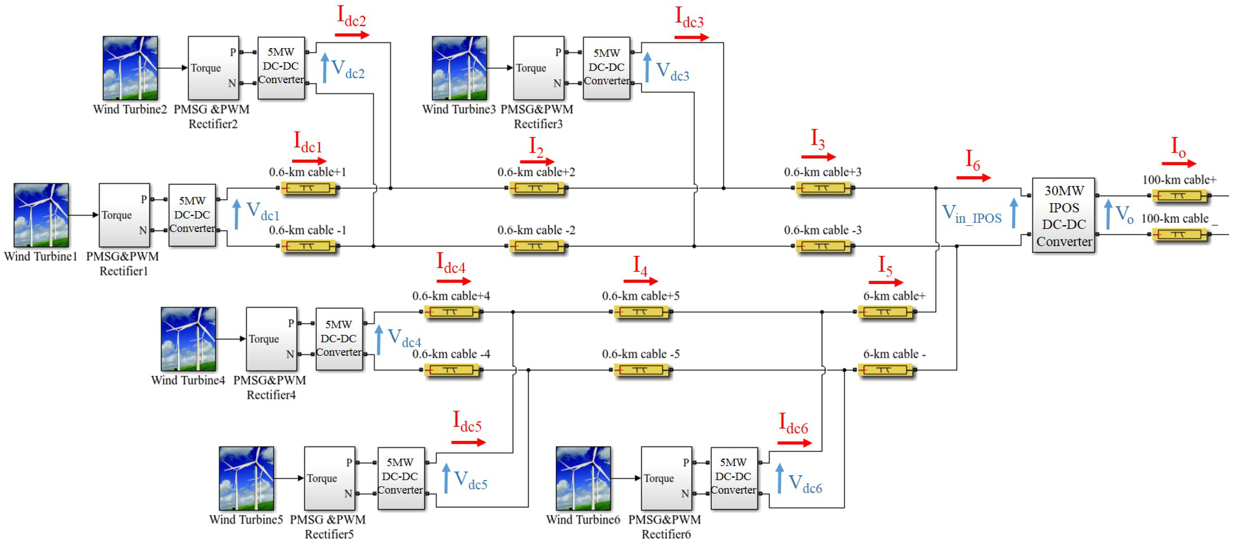
Figure 2.
Cable model.
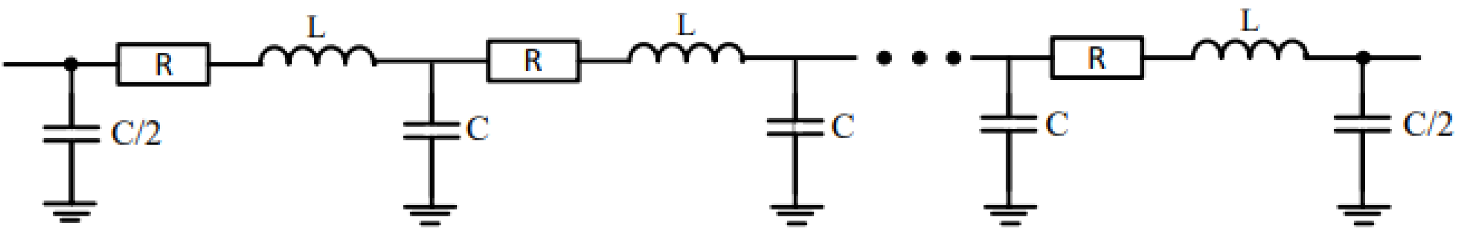
Figure 3.
Wind farm with circular structure.
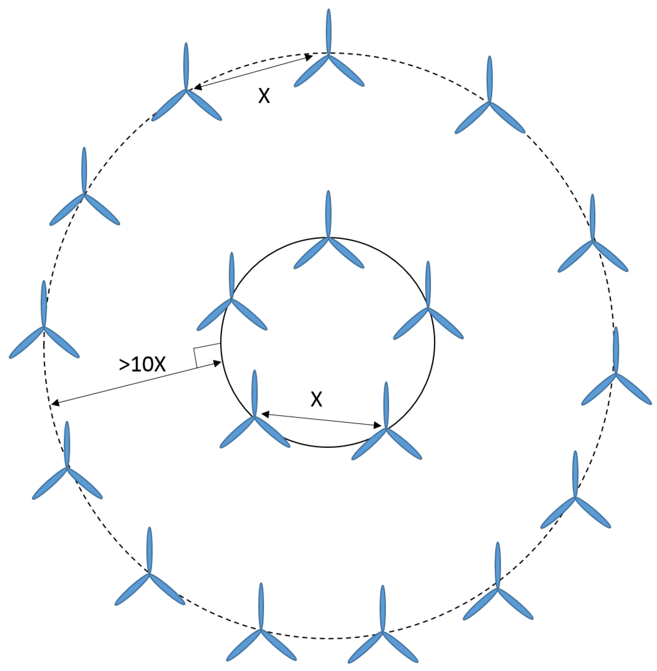
Figure 4.
Wind speed under wind condition 1.
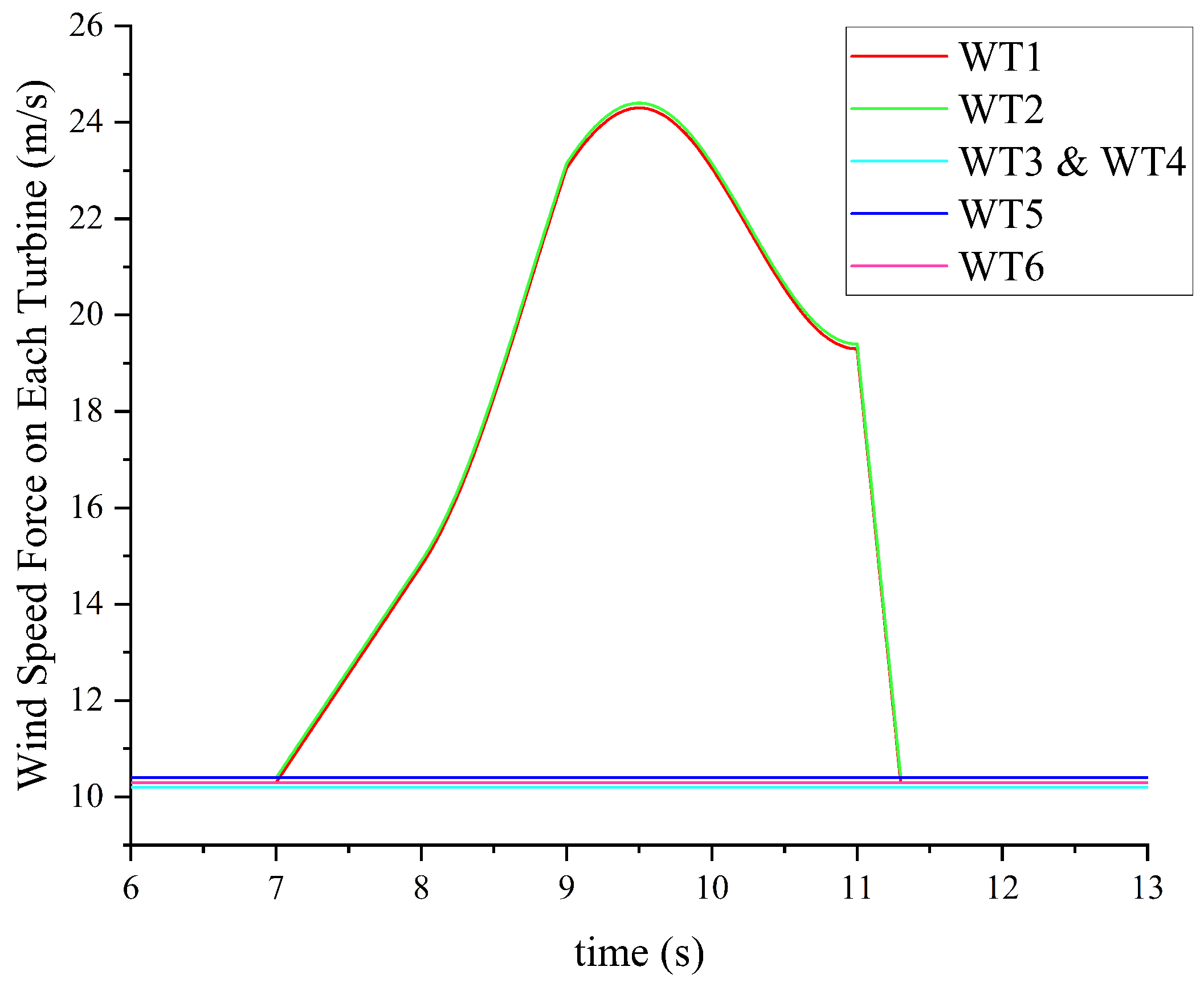
Figure 13.
Vdc1 and Idc1 with Identical Three-Phase IPOS structure.

Figure 14.
Wind condition 2.
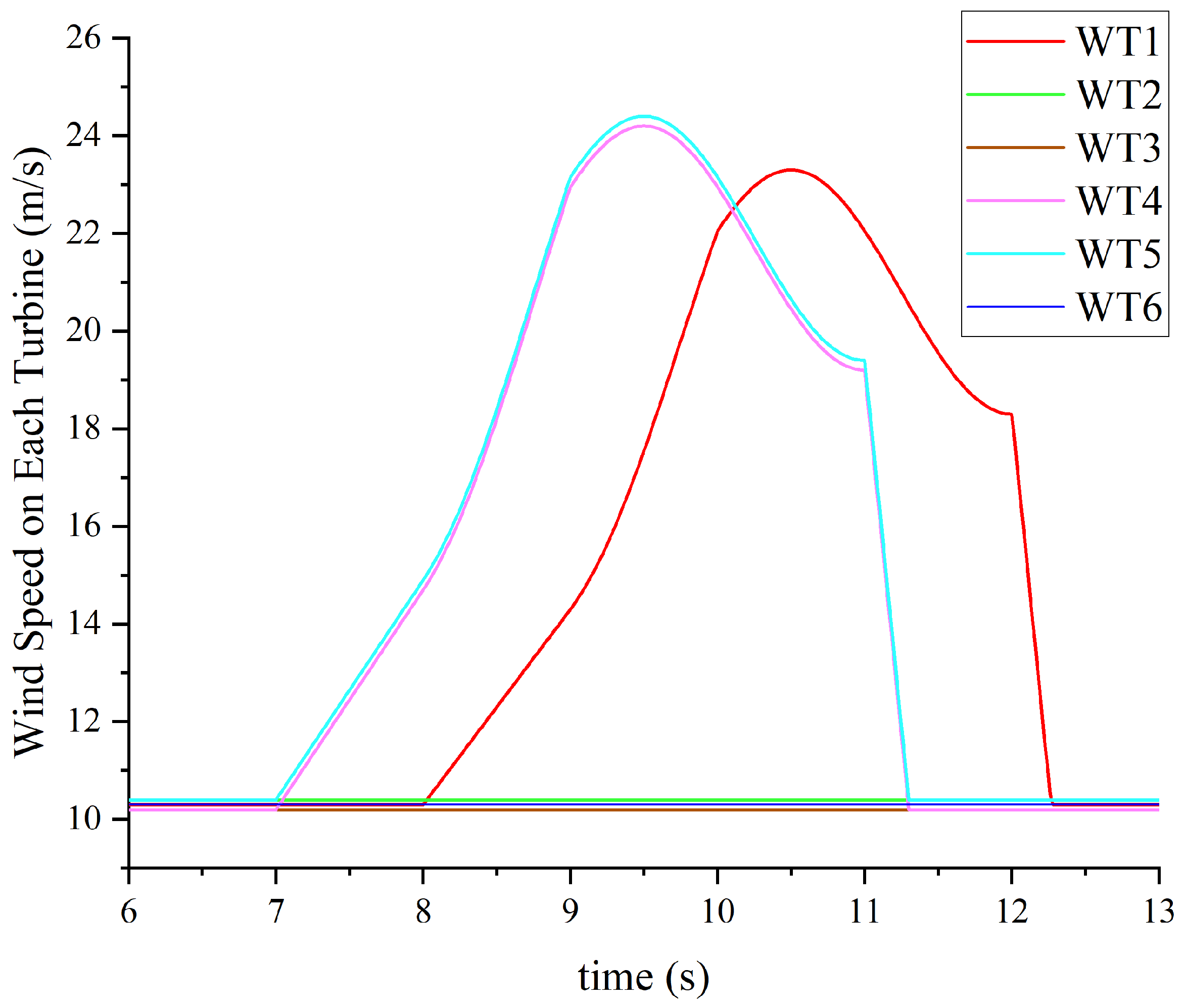
Figure 15.
Waveforms of Vdc1 and Idc1 under wind condition 2.

Figure 16.
Wind condition 3.

Figure 17.
Waveforms of Vdc1 and Idc1 under wind conditon 3.
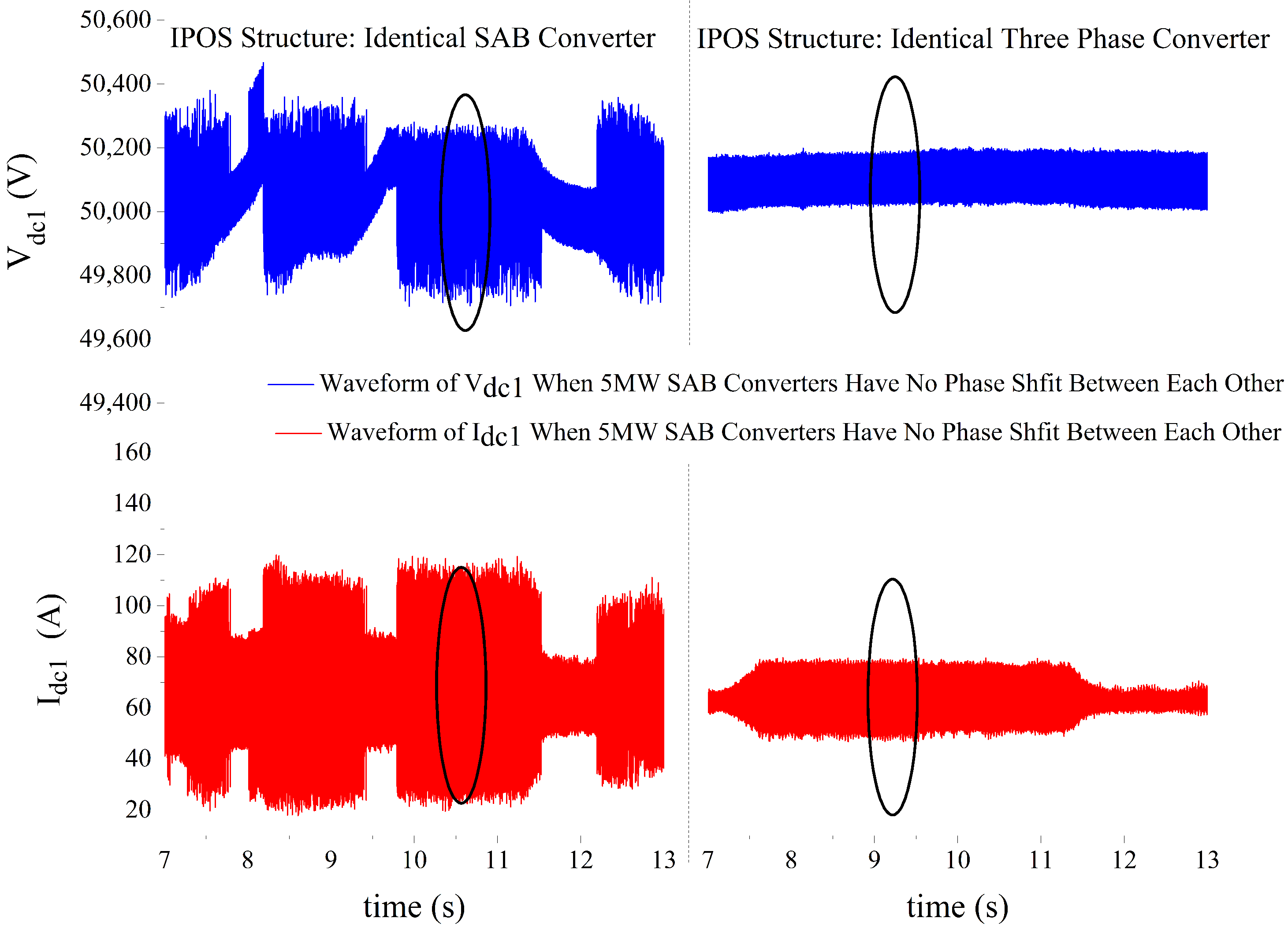
Figure 18.
Wind condition 4.
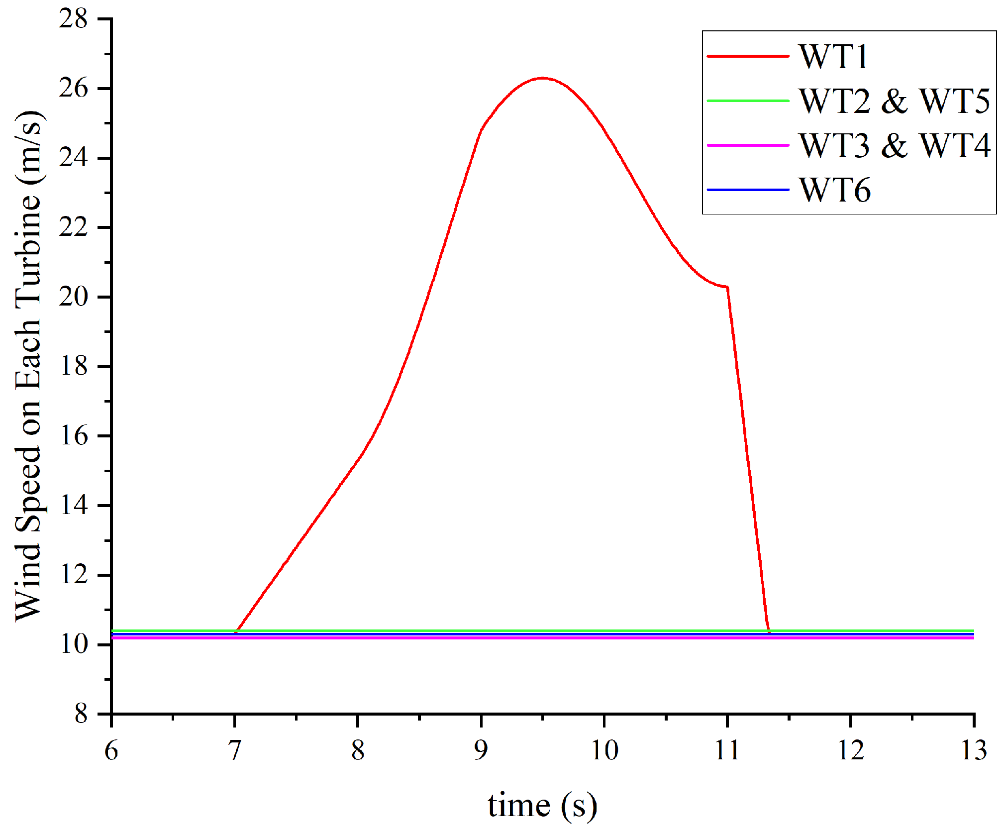
Figure 19.
Terminal voltages of system around cut-off time zone.

Figure 20.
Cable currents of system around cut-off time zone.
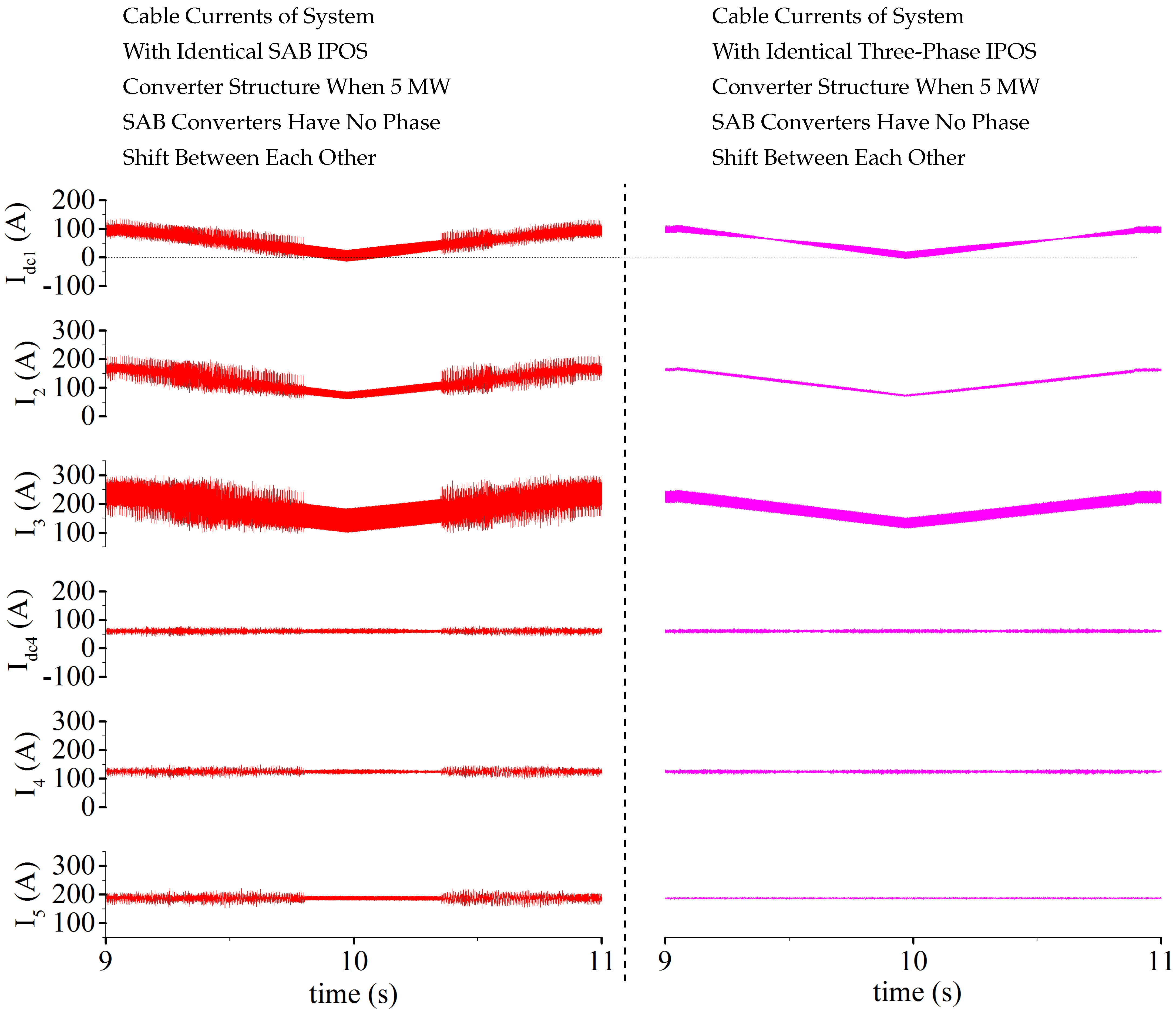
Figure 21.
Waveforms of Vo and Io around cut-off time zone.
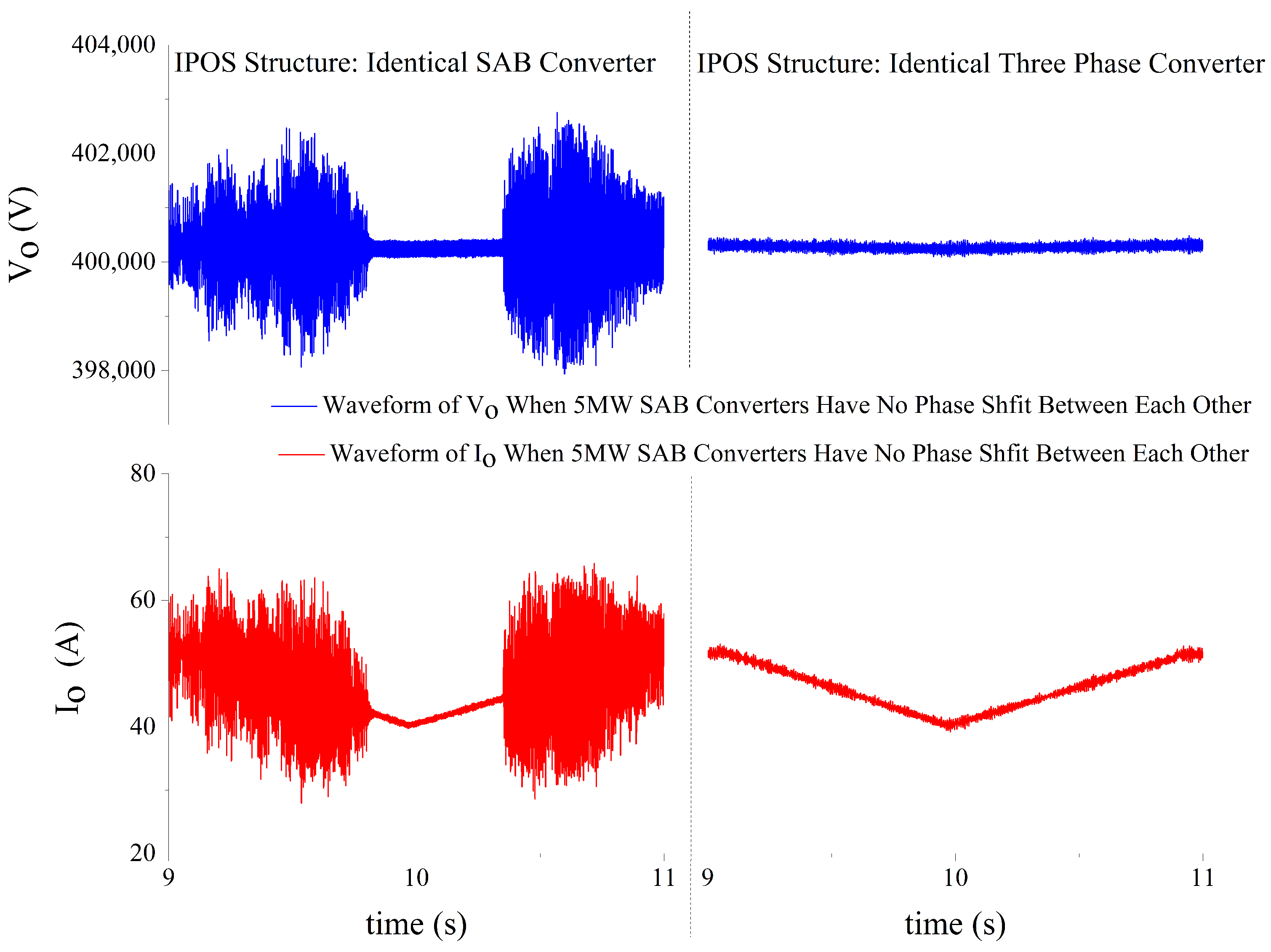
Table 1.
WT specification.
| Wind Turbine (WT) | |||||
|---|---|---|---|---|---|
| Type | Power Rating | Cut-In Wind Speed | Cut-Out Wind Speed | Rated Wind Speed | Nominal Rotation Speed |
| AD5135 | 5 MW | 5 m/s | 25 m/s | 12 m/s | 12 rpm |
Table 2.
PWM rectifier specification.
| Pulse Width Modulation Rectifier (PWM Rectifier) 1 | |||
|---|---|---|---|
| Vline_rms | Iline_rms | Power Rating | Output DC Voltage |
| 2.6 kV | 1.1 kA | 5 MW | 5 kV |
1 AC–DC converter connected after the PMSG.
Table 3.
5 MW DC–DC converter specification.
| 5 MW DC–DC Converter 1 | ||||
|---|---|---|---|---|
| Converter Type | Input Voltage | Output Voltage | Power Rating | Switching Frequency |
| Single Active Bridge (SAB) | 5 kV | 50 kV | 5 MW | 2 kHz |
1 DC–DC converter connected after the PWM rectifier to step up the voltage from 5 kV to 50 kV before the multi-terminal connection.
Table 4.
ISIPOS DC–DC converter specification.
| Input Series Input Parallel Output Series (ISIPOS) DC–DC Converter * | ||||
|---|---|---|---|---|
| Converter Type | Input Voltage | Output Voltage | Power Rating | Switching Frequency |
| Identical Three-Phase ISIPOS converter OR Identical SAB ISIPOS converter OR SAB+Three-Phase ISIPOS converter | 50 kV | 400 kV | 200∼1000 MW (reduced to 30 MW in this simulation work) | SAB converter: 2 kHz Three-Phase converter: 667 Hz |
* Collect the power from the wind farm and step up the voltage from 50 kV to 400 kV before the long-distance transmission to the shore.
Table 5.
±25 kV DC cable specification.
| ±25 kV DC Cables 1 | ||
|---|---|---|
| Cable Length of Each Branch | Power Rating of the Cable of Each Branch | Cable RLC Parameters |
| 0.6x km (x is the number of turbines in each branch | 5x MW | R = 60 m/km L = 0.3 mH/km C = 0.2 F/km |
1 Connected between multiple Turbine + PMSG + PWM + 5 MW DC–DC converter blocks to ISIPOS DC–DC converter.
Table 6.
±200 kV DC Cable Specification.
| ±200 kV DC Cables 1 | ||
|---|---|---|
| Cable Length | Power Rating of the Cable | Cable RLC Parameters |
| 100 km | 5y MW (y is the number of turbines in the whole offshore wind farm) | R = 30 m/km L = 0.8 mH/km C = 0.13 F/km |
1 Long submarine transmission cables connected between ISIPOS DC–DC converter and onshore power system.
Table 7.
Comparison of the THD of terminal voltages and Total Relative AC Losses on cables under different natural wind conditions.
Table 7.
Comparison of the THD of terminal voltages and Total Relative AC Losses on cables under different natural wind conditions.
| Base Value: Vdc = 50 kV Power = 3.2 MW Idc = 63 A 5 MW SAB Output Capacitor Value: 40 F IPOS Converter Input Capacitor Value: 0.4 F (TP) or 4 F (SAB) | ||||||
|---|---|---|---|---|---|---|
| WC 1 | WC 2 | WC 3 | ||||
| SAB | TP | SAB | TP | SAB | TP | |
| THD Vdc1 (%) | 0.3 | 0.15 | 0.32 | 0.17 | 0.26 | 0.14 |
| THD Vdc2 (%) | 0.3 | 0.18 | 0.31 | 0.13 | 0.26 | 0.19 |
| THD Vdc3 (%) | 0.27 | 0.15 | 0.29 | 0.16 | 0.26 | 0.2 |
| THD Vdc4 (%) | 0.19 | 0.15 | 0.23 | 0.16 | 0.18 | 0.17 |
| THD Vdc5 (%) | 0.19 | 0.15 | 0.27 | 0.16 | 0.19 | 0.16 |
| THD Vdc6 (%) | 0.18 | 0.15 | 0.26 | 0.15 | 0.17 | 0.16 |
| THD Vin_IPOS (%) | 0.51 | 0.03 | 0.51 | 0.03 | 0.52 | 0.03 |
| TRL-MS | 7.5 k | 0.8 k | 8.9 k | 0.9 k | 7.8 k | 1.8 k |
Table 8.
Comparison of the final output voltage, current and Relative Losses on a 100-km cable under different natural wind conditions.
Table 8.
Comparison of the final output voltage, current and Relative Losses on a 100-km cable under different natural wind conditions.
| Base Value: Vdc = 400 kV Power = 18.9 MW Idc = 47 A 5 MW SAB Output Capacitor Value: 40 F IPOS Converter Input Capacitor Value: 0.4 F (TP) or 4 F (SAB) | ||||||
|---|---|---|---|---|---|---|
| WC 1 | WC 2 | WC 3 | ||||
| SAB | TP | SAB | TP | SAB | TP | |
| THD Vo (%) | 0.28 | 0.2 | 0.38 | 0.02 | 0.32 | 0.01 |
| 100 kmTL | 90 | 0.32 | 92 | 0.9 | 92 | 1 |
| 100 | 4.2 k | 15 | 4.3 k | 42 | 4.3 k | 46 |
| Io(DC)/Ibase (%) * | 119 | 119 | 123 | 129 | 140 | 139 |
* The value of Io(DC)/Ibase (%) indicates the power generating ability, not the direct efficiency, of the system. It is calculated when all the turbines are operating under their maximum power region during the simulation period.
Disclaimer/Publisher’s Note: The statements, opinions and data contained in all publications are solely those of the individual author(s) and contributor(s) and not of MDPI and/or the editor(s). MDPI and/or the editor(s) disclaim responsibility for any injury to people or property resulting from any ideas, methods, instructions or products referred to in the content. |
© 2024 by the authors. Licensee MDPI, Basel, Switzerland. This article is an open access article distributed under the terms and conditions of the Creative Commons Attribution (CC BY) license (https://creativecommons.org/licenses/by/4.0/).
Share and Cite
MDPI and ACS Style
Rong, X.; Shek, J.K.H.; Macpherson, D.E.; Mawby, P. The Study of Multi-Terminal DC Systems in an Offshore Wind Environment: A Focus on Cable Ripple Analysis. Energies 2024, 17, 1978. https://doi.org/10.3390/en17081978
AMA Style
Rong X, Shek JKH, Macpherson DE, Mawby P. The Study of Multi-Terminal DC Systems in an Offshore Wind Environment: A Focus on Cable Ripple Analysis. Energies. 2024; 17(8):1978. https://doi.org/10.3390/en17081978
Chicago/Turabian StyleRong, Xiaoyun, Jonathan K. H. Shek, D. Ewen Macpherson, and Phil Mawby. 2024. "The Study of Multi-Terminal DC Systems in an Offshore Wind Environment: A Focus on Cable Ripple Analysis" Energies 17, no. 8: 1978. https://doi.org/10.3390/en17081978
Note that from the first issue of 2016, this journal uses article numbers instead of page numbers. See further details here.