
Wind Turbine Tower State Reconstruction Method Based on the Corner Cut Recursion Algorithm
School of Mechatronic Engineering and Automation, Shanghai University, Shanghai 200444, China
*
Author to whom correspondence should be addressed.
Energies 2024, 17(8), 1979; https://doi.org/10.3390/en17081979
Submission received: 14 August 2023
/
Revised: 16 April 2024
/
Accepted: 18 April 2024
/
Published: 22 April 2024
(This article belongs to the Section A3: Wind, Wave and Tidal Energy)
Abstract
:This study introduces an innovative approach for the reconstruction of wind turbine tower states using a tangential recursion algorithm. The primary objective is to enable real-time monitoring of the operational condition of wind turbine towers. The proposed method is rooted in strain–load theory, which enables the accurate identification of tower load states. The tangential recursion algorithm is utilized to translate the strain data acquired from strategically placed sensors into reconstructed point positions. The subsequent refinement of these positions incorporates considerations of torsional loads and geometric deformations, culminating in the comprehensive and precise reconstruction of the tower’s deformation behavior. Through the use of the OpenFAST V8 simulation software, a thorough analysis is conducted to investigate the load and deformation characteristics of the NREL 5 MW wind turbine tower across diverse operational scenarios. Furthermore, the load conditions corresponding to rated operating circumstances are applied to a finite element model constructed with the lumped mass method. The identification of tower load states and the comprehensive reconstruction of deformation patterns are realized through the extraction of strain data from critical points in the finite element model. The credibility and accuracy of the proposed method are rigorously evaluated by juxtaposing the identification and reconstruction outcomes with the results derived from the OpenFAST simulations and finite element analyses. Notably, the proposed method circumvents the requirement for external auxiliary calibration equipment for the tower, rendering it adaptable to a broader spectrum of operational contexts and making it consistent with unfolding trajectories in wind power advancement.
1. Introduction
Wind energy is considered to be one of the promising forms of renewable energy and has attracted significant attention over the past few decades due to its sustainability and feasibility [1]. The reliability of wind turbines plays a crucial role in the success of wind farm projects, and associated factors are essential for reducing energy costs [2]. In 2021, the newly installed wind power capacity in Europe reached a historical high of 17.4 GW, with a cumulative installed capacity of 236 GW [3]. From 2020 to 2022, China’s newly installed wind power capacity was 54.43 GW, 55.92 GW, and 49.83 GW, respectively, with a cumulative capacity reaching 370 GW [4].
Traditional wind power systems consist of three fundamental constituents: wind turbine generators, structural support frameworks, and transmission control mechanisms. As one of the three major systems, wind turbine foundations provide critical support for the entire wind turbine unit for at least 25 years and determine the safety, reliability, and stability of wind turbine units. During the actual operation of wind turbine towers, frequent tower collapses have been observed due to excessive loads and deformations, leading to significant economic losses and environmental damage. According to a research report on wind turbine tower collapses by the University of Birmingham in 2019, among the 47 incidents that occurred in Europe, America, and East Asia from 2000 to 2016, 55.7% were primarily caused by excessive tower deformations and overloading due to typhoons and storms [5]. In 2021, Gürdal Ertek collated data on wind turbine accidents since 2010 and carried out extensive research on the association between the phase of the wind turbine’s life cycle and the frequency of accidents, the association between death and injury and the phase of the life cycle, and the association between death and injury and the location (offshore vs. onshore) of the turbine [6]. Therefore, the identification and reconstruction of the load and the deformation states of wind turbine towers hold crucial practical significance. Numerous scholars have carried out extensive research on the measurement of wind turbine tower loads and deformations. In the domain of load studies, in 2005, Takeshi Ishihara from the University of Tokyo conducted an analysis of the wind turbine accident on Miyako Island caused by Typhoon Maemi and identified that the main cause of the tower collapse was the exceeding of the critical bending moment [7]. In 2015, Jui-Sheng Chou from National Taiwan University summarized the failure accidents of seven wind turbine towers in Taiwan caused by Typhoon Soudelor. Through employing finite element analysis, he investigated the failure mechanisms and structural weaknesses leading to the tower collapse and proposed improvement methods for anti-wind performance [8]. In the same year, Xiao Chen from the Chinese Academy of Sciences presented an analytical model to calculate the degree of tower structural damage under extreme wind loads [9]. Regarding deformation studies, in 2012 Hyung-Joon Bang utilized ten fiber optic grating sensors arranged on the inner surface of the tower’s main wind direction to measure the tower deflection through a strain–displacement transformation matrix [10]. In 2017, Gino B. Colherinhas from the University of Brasilia analyzed the displacement situation at the top of the tower using genetic algorithms and tuned mass dampers [11]. However, these methods only focused on the local structures of wind turbine towers and failed to represent the overall deformation situation. In 2021, Paula Helming from the University of Bremen employed a ground-based laser scanner with a horizontal alignment line scanning mode to measure the tower and determined its axial and lateral deformation results through a least square fitting approach [12]. In 2023, Andreas Baumann-Ouyang from ETH Zürich used synthetic aperture radar to identify the tower’s main frequency and to measure its deformation state [13]. These measurement methods require external auxiliary equipment and have high environmental requirements.
This study proposes a wind turbine tower load and deformation state reconstruction method based on the tangential recursion algorithm, which improves the accuracy of tower state reconstruction. Specifically, the method includes the following steps: (1) Based on the equations for bending moment and torsional load identification in the tower structure, the strain information obtained from sampling points is separated to extract the bending strain and torsional strain information endured by the tower structure, thereby achieving bending and torsional load identification. (2) The strain caused by bending is transformed into curvature information on the measurement points. Through combining the principles of bending sensing with the tangential recursion algorithm, the reconstructed information on the tower’s positions along the meridional direction at 0°, 90°, 180°, and 270° is obtained. (3) Using the torsional angle obtained from the torsional load identification, it is converted into circumferential displacement changes in the measurement points. Subsequently, the deformation reconstruction model obtained in step (2) is optimized to obtain the new coordinates of the measurement points.
In pursuit of the operationalization of the aforementioned methodology, a comprehensive array of investigations was carried out, the structural delineation of which is systematically elucidated as follows. Commencing with a comprehensive exposition of the foundational principles underpinning OpenFAST simulation analysis, tower bending moment and torsional load identification, strain–curvature conversion for the purpose of tower deformation reconstruction, the nuanced secondary interpolation methodology, and the intricate corner cut recursion algorithm, this research endeavors to propose a comprehensive methodology encompassing the meticulous extraction of external loads using the OpenFAST framework. This is conducted in tandem with the utilization of the corner cut recursion algorithm for the purpose of wind turbine tower deformation reconstruction (Section 2). Immediately afterwards, rigorous validation of the proposed external load extraction methodology using OpenFAST is conducted, which entails the configuration of the tower’s parameters within the context of the wind turbine model employed in the OpenFAST simulation milieu, a complete exposition of the operational tenets governing TurbSim, the purposive generation of turbulent wind fields germane for simulation imperatives, and the systematic orchestration of OpenFAST to simulate tower load and deformation dynamics across a spectrum of wind speeds and typologies. This procedure culminates in the articulation of a standardized framework for characterizing the external loading milieu within the context of finite element simulation (Section 3). The subsequent phase of the research trajectory pivots towards the validation of an authoritative simulation of a representative tower structure. This entails the instantiation of a finite element model tailored to the tower’s structural characteristics, the partitioning of mesh domains, the superimposition of externally computed load outcomes from the OpenFAST simulation onto the tower’s framework, the extraction of pivotal positional data from computed displacement and strain topography, and the rigorous realization of tower load identification and consequent reconstruction. This procedure culminates in a synthesized amalgamation of outcomes (Section 4). To complete this investigation, a comparative analysis is executed, which harmonizes the OpenFAST simulation results, finite element simulation outputs, and the emergent outcomes of the model’s identification and reconstruction. Through a tailored analysis, the integrity and efficacy of the formulated methodology are underscored and affirmed (Section 5). To complete the study presented in this paper, the culminating synthesis and inferences derived from the research findings are presented in Section 6.
2. Theoretical Basis
2.1. OpenFAST Simulation Principle
2.1.1. OpenFAST Operating Principle
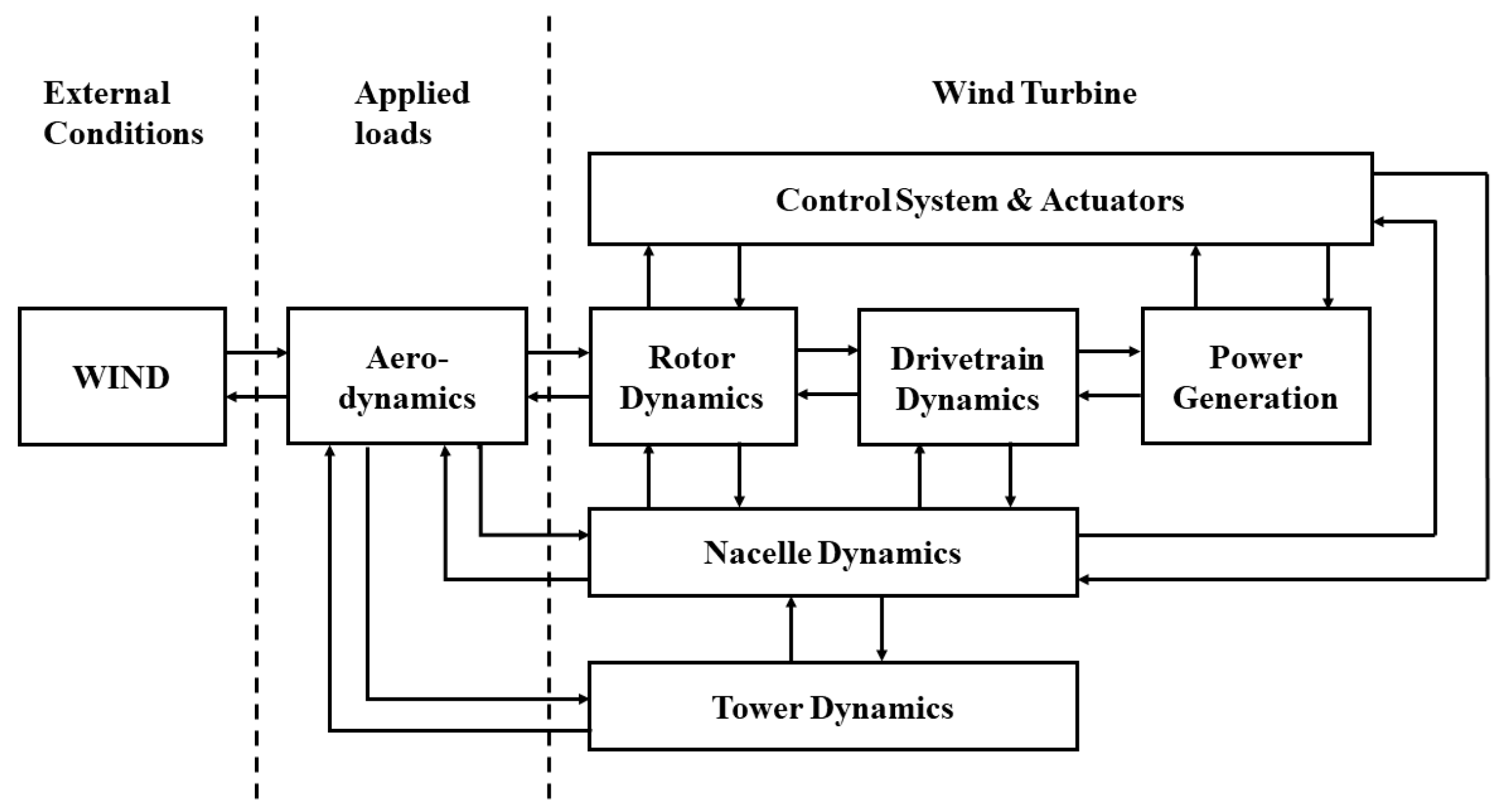
The OpenFAST wind turbine simulation software, developed and maintained by the National Renewable Energy Laboratory (NREL) in the United States, is a multi-module coupled simulation software system that enables the analysis of wind turbine operation. The simulation process is illustrated in Figure 1. Through iteratively refining the wind configuration documentation, adjusting the aerodynamics documentation, and precisely tailoring the wind turbine control documentation, a comprehensive framework for simulating wind turbine operation is systematically established. This calibration process yields intricate tower motion and load data throughout the wind turbine simulation. The extracted load outcomes subsequently serve as the foundational basis for the prescribing of external load conditions within the domain of finite element simulation.
2.1.2. Simulation Result Extraction Principle
In response to the distinctive characteristics of external load patterns acting upon wind turbine towers, this study devises a method that amalgamates outcomes from OpenFAST simulations with the dynamic load application within a finite element model of the tower. This integration yields a novel approach for extracting external load conditions for the subsequent finite element simulations, leveraging the data generated through OpenFAST simulations. The procedural framework, which is shown in Figure 2, is carried out as follows: (1) the selection of an appropriate wind turbine model within the OpenFAST environment, accompanied by tailored modifications to geometric attributes, material specifications, and control strategies; (2) the rigorous specification of simulation prerequisites, encompassing nuanced factors such as wind field characteristics, operational conditions, simulation temporal parameters, and computational time increments; (3) the comprehensive delineation of the tower’s geometrical properties, mass distribution, and structural stiffness within the wind turbine model, thereby facilitating the computational analysis of tower dynamics within the simulation domain; (4) the execution of dynamic simulations using OpenFAST, wherein the software performs intricate dynamic calculations of the wind turbine’s behavior, culminating in the determination of tower load distributions; and (5) the methodical retention of the computed load profiles at distinct tower elevations during the simulation process, thereby establishing a repository of load data for subsequent analysis and integration with finite element simulations.
2.2. Load Identification Principle of Tower
2.2.1. Bending Moment Identification Principle of Wind Turbine Tower
Under the influence of bending moment M, the circumferential and axial stress–strain relationship of the tower at any cross-section can be represented as [14], as illustrated in Figure 3:
In the equation, εxi represents the circumferential strain at any height section of the tower, σxi represents the circumferential stress at any height section of the tower, εyi represents the axial strain at any height section of the tower, σyi represents the axial stress at any height section of the tower, ν denotes the Poisson’s ratio of the tower material, and E represents the elastic modulus of the tower material. The index i represents the sensor number of a single profile at any height of the tower, ranging from 1 to n.
The calculations are obtained by evaluating Equations (1) and (2):
In accordance with the axial stress, the bending moment M can be formulated as:
In the equation, ϕi signifies the angular displacement between the sensor positioned at any given height and the initial sensor, where D signifies the outer diameter of the tower, and d signifies the inner diameter of the tower.
Through the application of the least squares fitting technique to Equation (4), the magnitude of the bending moment M experienced at the measured height of the tower can be determined as follows:
2.2.2. Torque Identification Principle of Wind Turbine Tower
Under the action of external loads on the tower, a torque of magnitude T is induced at the measured height, giving rise to shear stress and shear strain.
The shear strain γi is synthesized from the linear strain relationship:
Based on the strain relationship, the shear stress τ can be obtained:
The torque T can be calculated using Equations (6) and (7):
2.3. Deformation Reconstruction Method of Wind Turbine Tower
2.3.1. Principle of Curvature Reconstruction
The deformation reconstruction method investigated in this study is based on the iterative estimation of curvature information. To achieve this, it is essential to convert the strain measurements at specific locations into their corresponding curvatures. Carefully selecting a segment of the structure for analysis, the underlying principle of bending sensors is illustrated in Figure 4.
To examine the undeformed state, let us consider a microelement with a length of L and a height of h, as illustrated in Figure 4a. Upon the application of a bending moment M, the upper surface of the microelement experiences tensile deformation, while the lower surface undergoes compressive deformation. By virtue of the continuous nature of deformation, a neutral layer exists between the tensile and compressive regions, wherein the length remains unchanged. This neutral layer possesses a curvature radius denoted as ρ, as depicted in Figure 4b. Hence, the curvature of the neutral layer serves as a means to characterize the geometrical transformation of the microelement. From Figure 4b, we can deduce the following relationship:
In the aforementioned equation, ΔL denotes the variation in length of the structural microelement, while θ represents the central angle associated with the corresponding arc during the deformation of the microelement.
Utilizing Equations (9) and (10), a correlation can be established between the curvature k of the microelement and the strain ε, as expressed by the following relationship:
2.3.2. Interpolation Algorithm
In practical monitoring scenarios, where strain measurements are limited to a finite number of points along a curve, it becomes necessary to interpolate the curvature values in order to reconstruct the complete shape of the curve. This interpolation is based on the assumption that the curvature varies non-uniformly between adjacent points. To achieve this, a quadratic function is employed to establish the relationship between the curvature (k) and the corresponding arc length (s) along the curve. Fitting this quadratic function to the available strain data, the curvature at any desired point along the curve can be estimated, enabling a comprehensive reconstruction of the curve’s shape.
In the equation, M, N, and Q represent the coefficients of the quadratic function. These coefficients determine the shape and characteristics of the quadratic curve that approximates the relationship between curvature (k) and arc length (s).
Partitioning the curve into contiguous arc segments of equal length, denoted as S1~S2, S2~S3, … Sn~Sn+1, Sn+1~Sn+2, we can establish the following relationships:
Utilizing the provided data on curvature and arc length, the numerical values of the coefficients M, N, and Q can be computed, enabling the construction of quadratic functions. This mathematical framework allows the extrapolation of curvature information to additional points along the curve, thereby enhancing the scope and accuracy of the curvature analysis.
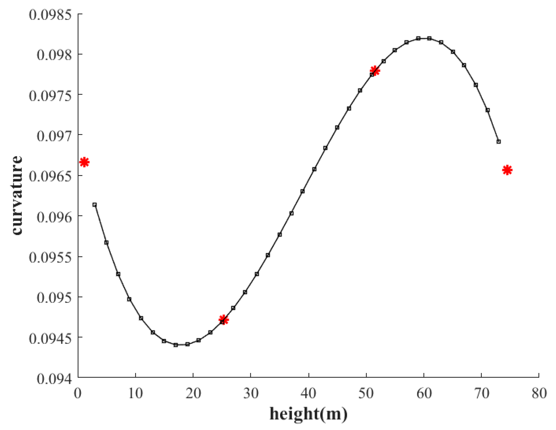
As shown in Figure 5, the red * marks represent the curvature sizes of the different heights measured using sensors, and the black dots represent the curvature sizes of the different heights obtained using the above interpolation algorithm; thus, the supplementary curvature information on the untested heights is complete and serves as the basis for reconstruction.
2.3.3. The Corner Cut Recursion Algorithm
When two points on a curve are sufficiently close, the curve between these points can be approximated as a small circular arc. The tangent recursion method is based on this assumption, where the coordinates of the next point are derived from the coordinates of the previous point, and this process is repeated to obtain the positions of all the points on the curve in a Cartesian coordinate system. For any arbitrary curve, as shown in Figure 6, consider the distance between two points on the curve as s. As the distance, s, approaches zero, this segment of the curve can be represented as a differential arc denoted as ΔSn. The starting point of the differential arc is denoted as On (Xn, Yn), and the endpoint is represented as On+1 (Xn+1, Yn+1). The curvatures at these points are denoted as Kn and Kn+1, respectively. The tangent vector at the starting point of the arc is denoted as α, ln represents the chord length of the differential arc, and ΔSn corresponds to the arc length between the two points. The angle Δθ represents the central angle associated with the arc ΔSn. Treating the curve as a sequence of differential arcs and applying the tangent recursion method, the coordinates of each point on the curve can be determined. This approach enables the reconstruction of the entire curve in a Cartesian coordinate system, allowing for the representation and analysis of the curve’s shape and position.
Based on Equation (13) and Figure 4, it can be deduced that the corner cut recursion algorithm computes the coordinates of successive points on a curve by iteratively applying the following formula:
2.4. Wind Turbine Tower Simulation Module Based on OpenFAST
The validation of the proposed methodology is conducted using the well-established 5 MW reference wind turbine model formulated by the National Renewable Energy Laboratory (NREL). This model stands as a quintessential representation of a three-bladed horizontal-axis wind turbine configuration. The key parameters governing its characteristics are meticulously presented in Table 1 and serve as a fundamental reference for the subsequent analytical investigation.
Through meticulous parameter-configuration-encompassing elements, such as the wind turbine model, atmospheric conditions, and simulation duration, a dynamic response simulation is executed within the OpenFAST computational framework. Subsequent to this simulation endeavor, the computed load and displacement outcomes are documented within the software’s ‘.out’ result files. It is worth noting that these load outcomes are destined to serve as the foundational loading conditions for the subsequent finite element simulations. Additionally, the displacement results are poised to undergo meticulous comparative analysis with respect to the tower deformation reconstruction outcomes derived from the methodology, which is reliant on the corner cut recursion algorithm.
2.5. Reconstruction and Optimization Method for Wind Turbine Tower Based on Corner Cut Recursion and Torque Load
2.5.1. Deformation Reconstruction Method for Wind Turbine Towers Based on Corner Cut Recursion
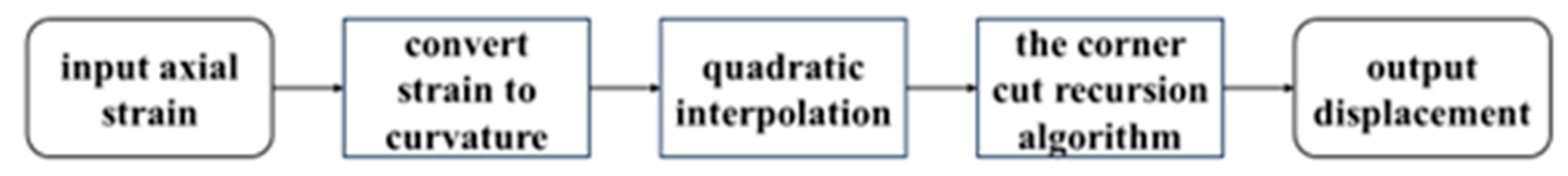
In this investigation, strain sensors were strategically installed at specific locations along the tower at heights of 1.1 m, 25.3 m, 51.5 m, and 74.5 m, corresponding to orientations of 0°, 90°, 180°, and 270°. The purpose was to capture the variations in axial strain along these positions, facilitating the reconstruction of tower deformation. The detailed methodology for the tower deformation reconstruction process is depicted in Figure 7.
According to Figure 8, the axial strain measurements at four designated sensor locations along the generatrix direction of the tower are converted into curvature values. These curvature values are interpolated using a quadratic interpolation algorithm to obtain an additional 12 equidistant curvature values between each pair of adjacent sensor locations. Subsequently, the interpolated curvature values, along with their corresponding arc lengths, are utilized in the corner cut recursion algorithm to calculate the two-dimensional displacement coordinates for each point along the tower.
2.5.2. Deformation Optimization Method for Wind Turbine Towers Based on Torque Information
The corner cut recursion algorithm provides two-dimensional coordinate variation results, which represent the displacement along the radial direction of the cross-sections. However, in real-world scenarios, the tower experiences torsional deformation due to torque loading, resulting in circumferential displacements. Thus, it is necessary to calculate the circumferential displacements and transform the reconstructed points from a two-dimensional plane variation to a three-dimensional spatial variation to achieve optimized results. To calculate the deflection angles of different tower sections, torque load information is utilized to determine the extent of the deformation.
In the equation, l represents the distance between two measurement points, G denotes the shear modulus, t represents the wall thickness, d1 refers to the diameter at the lower end of the tower section, and d2 represents the diameter at the upper end of the tower section.
Following the computation of the deflection angle φ for the tower section, it is commonly assumed that the mast axis remains linear even under small torsional deformations, as illustrated in Figure 9. Utilizing geometric principles, the circumferential displacements of the reconstructed points along the tower can be precisely derived.
Let us consider a point located within the cross-sectional area of the tower. Prior to deformation, this point is denoted as A (X, Z) in the undeformed configuration. However, under the influence of torsional deformation, it undergoes displacement and is relocated to point B (X′, Z′) in the deformed configuration. Applying geometric principles and calculations, we can determine the circumferential displacement of the reconstructed point along the circumference of the tower.
Upon acquiring the alterations in coordinates at various elevations of each tower segment, we can deduce the circumferential displacement at different heights of the tower. This enables us to ascertain the circumferential deformation across distinct sections of the tower.
After the tower undergoes bending and torsional deformation, the distance l between the sampling points remains unchanged. Let Y denote the vertical coordinate before deformation and Y’ denote the vertical coordinate after deformation. Based on geometric considerations, we can deduce the following academic and logical conclusions:
In the given equation, Δx denotes the displacement in the X-direction at a specific point, while Δz represents the displacement in the Z-direction at the same point. These variables quantify the changes in coordinates corresponding to the respective directions.
Incorporating the corrections, the coordinates (X′, Y′, Z′) accurately portray the precise location of the deformed tower in three-dimensional space. This revised coordinate system enables accurate measurement, analysis, and representation of the tower’s deformed geometry and spatial attributes.
3. Materials and Methods
3.1. Tower Load Application Model Based on FAST
The present study employs the 5 MW OC3 Mnpl DLL WTurb WavesIrr model provided by the OpenFAST simulation software for conducting comprehensive simulations. The specific procedural steps encompass setting of the geometric configuration, where tower parameters such as height, upper and lower diameters, and wall thicknesses are precisely defined. The material properties are rigorously specified and include material density, Young’s modulus, and the shear modulus. Additionally, the setup involves the establishment of distributed tower characteristics, including stiffness and mass matrices, as detailed in Table 2. This methodical configuration and the meticulous parameterization provide a solid foundation for subsequent simulations, ensuring the accuracy and rigor of the computational analyses conducted within this research.
The Paraview 5.12.0 software was employed to visually process the simulation model constructed within OpenFAST, yielding the results depicted in Figure 10. The finalized model, as showcased, is amenable to simulation computations under diverse operating conditions. This visualization step enhances the comprehensibility and applicability of the constructed model, facilitating its utilization in various scenarios of interest.
3.2. Generation of Turbulent Wind Fields Using TurbSim
TurbSim is a stochastic full-field turbulent wind time series modeling software system developed by NREL. It employs statistical models to generate a time series of wind speed vectors (u, v, w) at points within a two-dimensional vertical grid matrix, as illustrated in Figure 11. The bts files generated by TurbSim serve as inputs for the wind module and subsequently influence the data calculations in the aerodynamics module.
First, RandSeed1 was set to 19970818, RandSeed2 was set to RANLUX, NumGrid_Z was set to 11, NumGrid_Y was set to 10, GridHeight was set to 170, and GridWidth was set to 220. Then, the wind field simulation was conducted using the IEC Kaimal wind spectrum with the normal turbulence model (NTM) and a turbulence intensity level set to IEC-A. The purpose was to generate a turbulent wind field with a reference wind speed of 11.6 m/s, a maximum wind speed of 17 m/s, and a minimum wind speed of 5.38 m/s. The simulation results for the wind speed at hub height are illustrated in Figure 12, while the wind speed distribution across the entire domain is depicted in Figure 13. Overall, these simulation results, based on the IEC Kaimal wind spectrum and the NTM with a turbulence level set to IEC-A, demonstrate the generation of a turbulent wind field with a reference wind speed of 11.6 m/s, featuring varying wind speeds ranging from 5.38 m/s to 17 m/s at different locations within the domain.
3.3. Simulation Condition Design
Using the computational framework of OpenFAST, four distinct simulation scenarios were systematically employed, as outlined in Table 3. The initial three simulations were rigorously executed within a realm of steady-state wind conditions, featuring reference wind velocities of 3 m/s (corresponding to the cut-in wind speed), 11.6 m/s (representative of the rated wind speed), and 25 m/s (akin to the cut-out wind speed), respectively. The fourth simulation configuration encompassed the intricate dynamics of turbulent wind conditions, operating at a reference wind velocity of 11.6 m/s. Aiming to capture the entire temporal trajectory spanning from the turbine startup to the attainment of stable operational conditions, each simulation was allocated a temporal extent of 1800 s. This temporal allocation facilitated a comprehensive analysis of the tower’s nuanced load-bearing behavior and its dynamic motion responses across a diverse spectrum of operational contexts.
3.4. Analysis of Tower State Variation in Loads and Displacements under Different Wind Conditions
3.4.1. Analysis of Tower State Variation in Loads and Displacements at Different Heights under Steady-State Wind Conditions
Under the influence of steady-state wind conditions, the temporal evolution of the displacements at various heights of the tower during the LC1 operational scenario is graphically depicted in Figure 14. The pinnacle of the tower showcases the most prominent displacement, measuring 0.02559 m. Furthermore, the temporal trajectory of the bending moments experienced at different heights of the tower during the LC1 scenario is illustrated in Figure 15. The maximum bending moment occurs at the base of the tower, reaching a magnitude of 4791 kN·m, whereas the minimum bending moment is observed at the tower’s apex during the wind turbine’s startup phase, registering a magnitude of −1702 kN·m. As the operation attains a state of stability, the magnitudes of the tower displacements gradually increase with the height, while the magnitudes of the bending moments decrease in proportion to the increase in height.
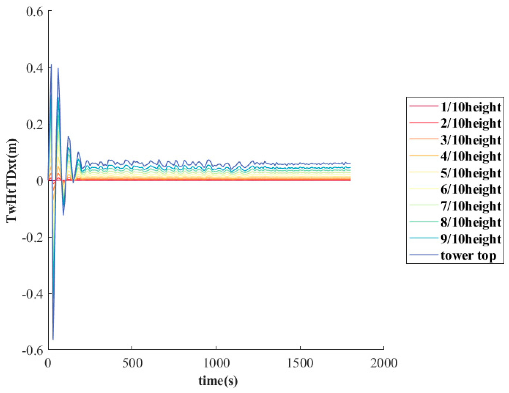
Under the influence of steady-state wind conditions, the temporal variations in the displacements at various heights of the tower during the LC2 operational scenario are presented in Figure 16. The tower’s pinnacle experiences the most significant displacement, measuring 0.375934 m. Similarly, the time-varying bending moments encountered at different heights of the tower during the LC2 scenario are depicted in Figure 17. The highest bending moment manifests at the tower’s base, reaching a magnitude of 58,630 kN·m, while the smallest bending moment is observed at the tower’s top, registering a magnitude of 27.69 kN·m. As the operational stability is reached, the magnitudes of the tower displacements progressively increase with height, while the magnitudes of the bending moments decrease proportionally to elevation.
Under the influence of steady-state wind conditions, the temporal variations in the displacements at various heights of the tower during the LC3 operational scenario are depicted in Figure 18. The apex of the tower exhibits the highest displacement, measuring 0.058679 m. Correspondingly, the time-dependent variations in the bending moments experienced at different heights of the tower during the LC3 scenario are illustrated in Figure 19. The maximum bending moment arises during the wind turbine startup phase at the tower’s base, reaching a magnitude of 87,390 kN·m. Conversely, the minimum bending moment during this startup phase is also observed at the tower’s base, with a value of −83,050 kN·m. Following the attainment of operational stability, the magnitudes of the tower displacements progressively increase with elevation, while the magnitudes of the bending moments decrease proportionally to height.
3.4.2. Analysis of Tower State Variation in Loads and Displacements at Different Heights under Turbulent-State Wind Conditions
Under the influence of turbulent wind conditions, the temporal variations in the displacements at various heights of the tower during the LC4 operational scenario are presented in Figure 20. Notably, the apex of the tower exhibits the maximum displacement, reaching a magnitude of 0.4764 m. This value demonstrates a notable increase of 25.13% compared to the maximum displacement observed under steady-state wind conditions at the same reference wind speed. Correspondingly, the time-dependent variations in the bending moments experienced at different heights of the tower during the LC4 scenario are depicted in Figure 21. The tower experiences its maximum bending moment at the base, measuring 7.30 × 10⁴ kN·m. This magnitude reflects an increase of 24.51% in comparison to the maximum bending moment observed under steady-state wind conditions at the same reference wind speed. Moreover, under turbulent wind conditions, the tower displacements progressively increase with height, while the magnitudes of the bending moments decrease proportionally to the increase in elevation.
3.5. Comprehensive Analysis and Summary of External Load Distribution on Wind Turbine Tower Structure
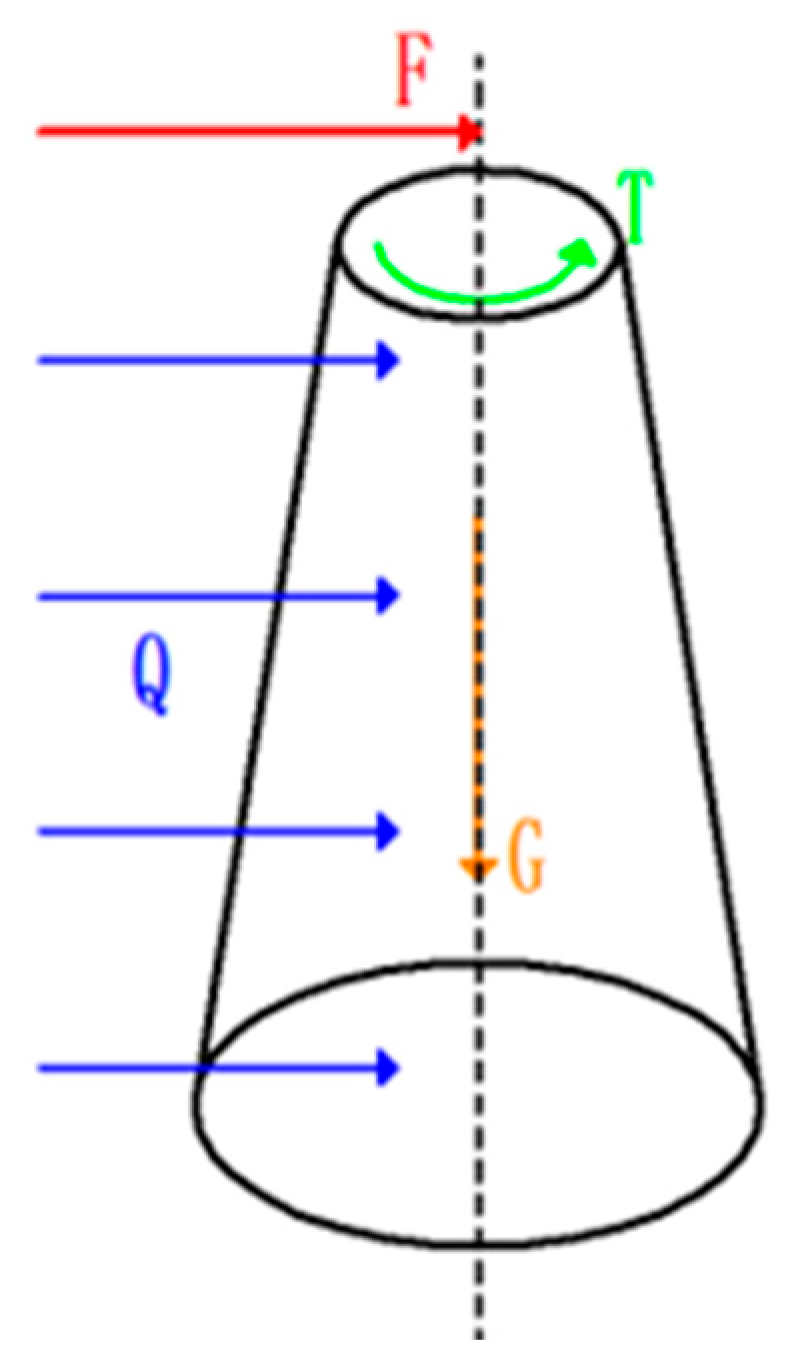
Through the utilization of the OpenFAST software for comprehensive analyses across diverse operational scenarios, the structural response of a large-scale wind turbine tower, designed with a varying cross-sectional thin-walled frustum configuration, is shown in Figure 22. This depiction encompasses the intricate interplay of both fixed and variable loading conditions. Specifically, the fixed loads encompass the gravitational influences originating from the blade ensemble, the nacelle, and the tower’s inherent mass. In contrast, the variable loading regime encapsulates the transference of lateral force, denoted as F, which is a consequence of wind-induced loading, exerted by the nacelle and blades. This lateral force magnitude reaches 7.2 × 10⁵ N when subjected to the rated wind speed conditions. Furthermore, the windward facade of the tower experiences a uniformly distributed wind load Q, attaining 61,630 N during the operation at the rated wind speed. Additionally, the rotational dynamics of the nacelle and blades engender a torque T that is conveyed to the tower’s upper extremity, measuring 5.256 × 10⁵ N·m under the stipulated rated wind speed. Evidently, the meticulously derived tower load data from the OpenFAST simulations constitute a pivotal input that facilitates the subsequent load imposition within the realm of the finite element simulations.
4. Finite Element Simulation Validation of Deformation Reconstruction and Optimization Method for Wind Turbine Towers Based on Corner Cut Recursion Algorithm
4.1. Model Building
4.1.1. Model Parameters and Mesh Partitioning in Finite Element Analysis
The model construction of the tower for the NREL 5 MW wind turbine is based on a three-section configuration with a total height of 77.6 m. The dimensional parameters of the tower are presented in Table 4, while the material properties of the tower are provided in Table 5.
The tower model of the wind turbine was established using the Ansys Workbench 2020r2 software, as illustrated in Figure 23. The method employed in this study involved applying the loads from components such as the nacelle and rotor to the tower using a lumped parameter approach, which was equivalently represented by a mass block at the top. The meshing of the model was performed as shown in Figure 24, with a total of 959,737 nodes and 440,839 elements. The element size was set to 0.2 m.
4.1.2. Load and Boundary Conditions in Structural Analysis
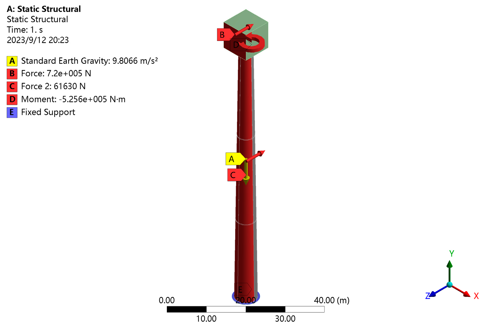
Through subjecting the tower to finite element simulations under the rated wind speed operational condition of LC2, a comprehensive investigation was undertaken to elucidate the imposed loads. In this analytical framework, the tower’s response is scrutinized under a composite load profile that encompasses not only its intrinsic gravitational load, which is attributable to its mass, but also those loads stemming from the nacelle and blades. Additionally, the tower contends with lateral wind forces transmitted by the nacelle and blades due to wind loading. Furthermore, the tower is subjected to the effects of uniform wind loads distributed across its windward surface and the torsional loads imposed by the nacelle onto the tower’s windward face during operational phases. This intricate amalgamation of forces, as depicted in Figure 25, is meticulously incorporated into the finite element simulation, providing comprehensive insights into the ensuing structural responses of the tower within the specific parameters of the LC2 operational regime.
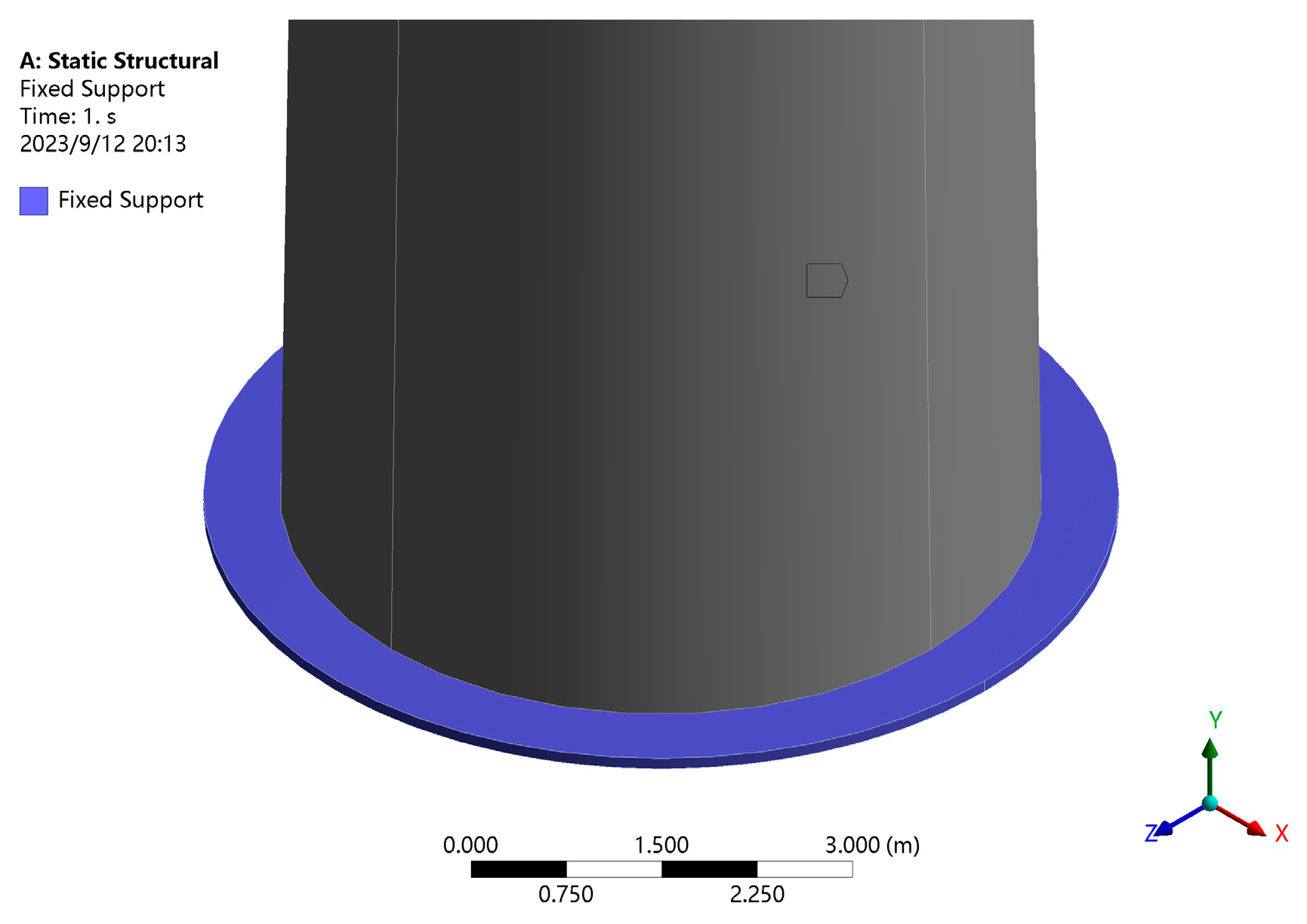
The connection between the tower base and the foundation is commonly established using a double-row bolted flange, which possesses superior strength compared to that of the other components. It is assumed that this flange remains undeformed, allowing for a fixed support configuration where the base flange surface is constrained in all six degrees of freedom, as illustrated in Figure 26.
4.2. Analysis of Simulation Results
4.2.1. Deformation Simulation Results
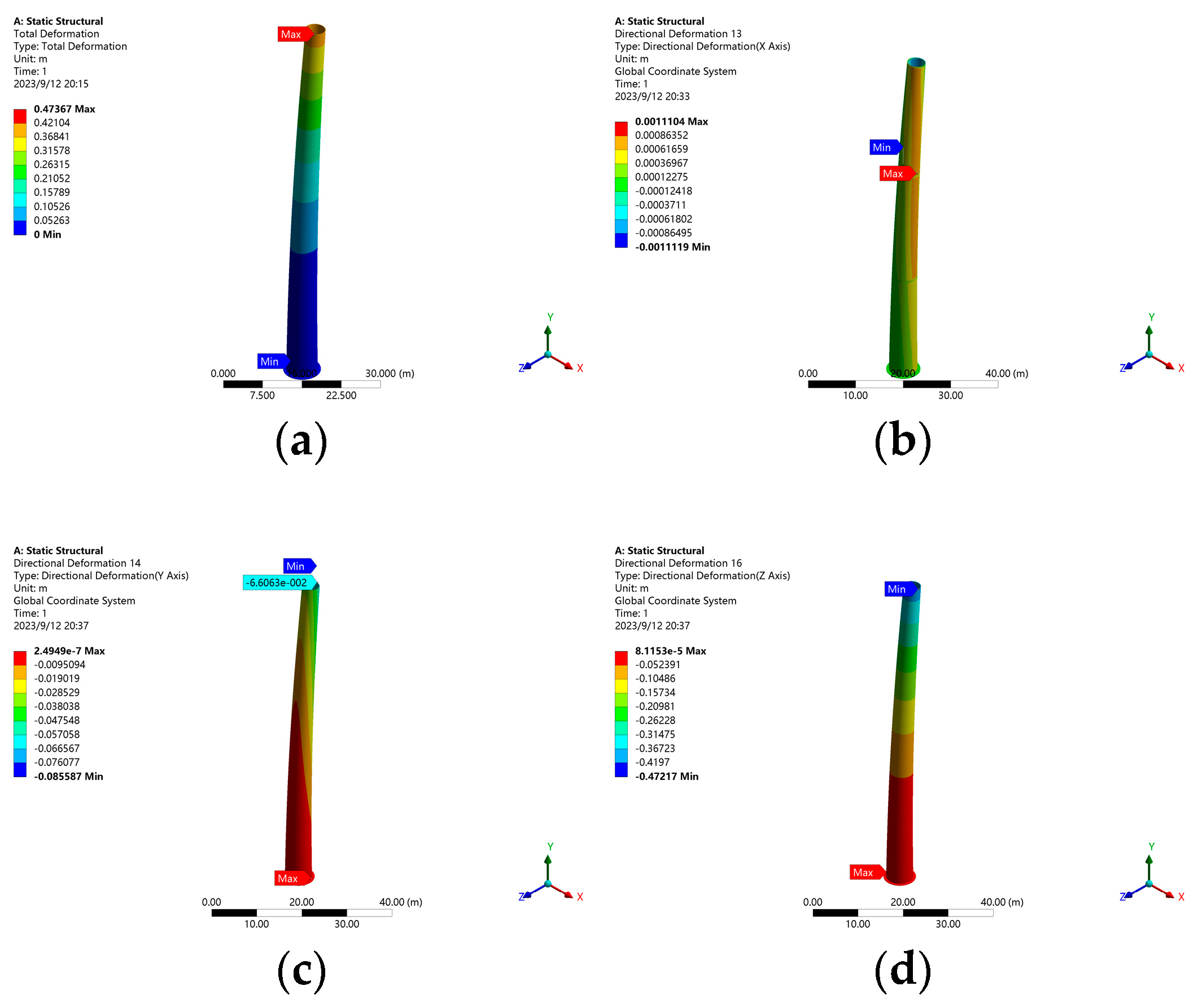
The simulation results are consistent with the expected results. The overall displacement results of the tower are shown in Figure 27a. The maximum overall displacement occurs at the top of the tower, with a magnitude of 0.40119 m, while the minimum overall displacement is at the bottom of the tower, with a magnitude of 0 m. The total displacement of the simulation model increases with increasing height. This indicates that the tower undergoes significant displacement at the top, while the bottom remains relatively stationary. The X-direction displacement results of the tower are presented in Figure 27b. The maximum displacement in the X-direction is observed near the connection between the upper and middle sections of the tower, with a value of 0.001104 m. Similarly, the minimum displacement in the X-direction also occurs near this connection, with a value of −0.001111 m. The displacement in the X-direction is basically symmetrical. This indicates that the tower experiences lateral displacement in the X-direction at this specific location. In terms of Y-direction displacement, as shown in Figure 27c, the maximum displacement occurs at the base of the tower, measuring 2.4949 × 10⁻⁷ m, while the minimum displacement is observed at the top of the tower, measuring −6.6062 × 10⁻² m. This indicates that the tower experiences vertical displacement, with the base moving slightly upwards and the top moving downwards. Basically, there is no displacement in the Y-direction. Lastly, the Z-direction displacement results are depicted in Figure 27d. The Z-direction is the main displacement direction. The maximum displacement in the Z-direction occurs at the tower base, measuring 8.1153 × 10⁻⁵ m, while the minimum displacement is observed at the tower top, measuring −0.39619 m. This indicates that the tower undergoes significant vertical displacement, with the base moving upwards and the top moving downwards. These displacement results contribute to the assessment of the tower’s structural performance and safety considerations.
4.2.2. Strain Simulation Results
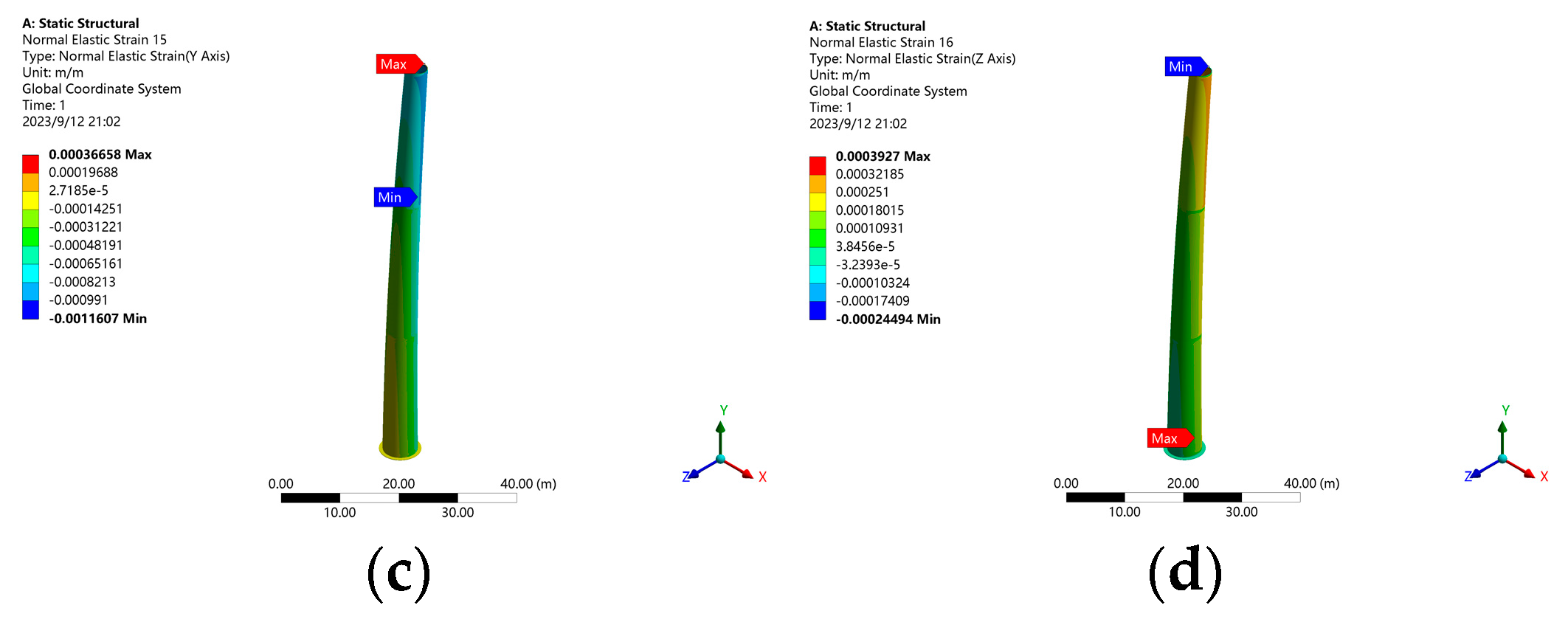
The simulation results for the strain closely align with our anticipated outcomes, with the peak strain concentrations consistently occurring at the junctions of individual tower components. Consequently, when extracting strain data, it is advisable to focus on the areas near the connection heights of each tower segment. The equivalent strain results of the tower are shown in Figure 28a. The maximum equivalent strain occurs near the connection between the upper and middle sections of the tower, with a magnitude of 1171.3 με, while the minimum equivalent strain is observed at the bottom of the tower, with a magnitude of 5.5607 × 10⁻⁶ με. This indicates that the tower experiences significant strain variations along its height. The X-direction strain results of the tower are presented in Figure 28b. The maximum strain in the X-direction is observed near the connection between the upper and middle sections of the tower, with a value of 363.99 με. Conversely, the minimum strain in the X-direction occurs at the top of the tower, with a value of −261.7 με. This indicates that the tower undergoes significant strain variations in the lateral direction. In terms of Y-direction strain, as shown in Figure 28c, the maximum strain occurs at the top of the tower, measuring 366.37 με, while the minimum strain is observed near the connection between the upper and middle sections of the tower, measuring −1160.7 με. This indicates that the tower experiences significant strain variations in the vertical direction, with compression at the top and tension near the connection region. Lastly, the Z-direction strain results are depicted in Figure 28d. The maximum strain in the Z-direction occurs at the tower base, measuring 392.7 με, while the minimum strain is observed at the tower top, measuring −243.12 με. This indicates that the tower undergoes significant strain variations in the vertical direction, with compression at the base and tension at the top. These strain results contribute to the evaluation of the tower’s structural integrity and provide valuable information for design optimization and maintenance considerations.
4.3. Load Identification Results
According to Equation (5), the computed bending moments for the tower are as follows: at the height of 1.1 m, the bending moment is 58,379.3 kN·m; at 25.3 m, it is 39,147.29 kN·m; at 51.5 m, it amounts to 18,324.14 kN·m; and at 74.5 m, it corresponds to 36.24 kN·m. Moreover, the torsional moments at these respective heights, as determined by Equation (8), are as follows: at 1.1 m, the torsional moment is 5.18 × 10⁵ kN·m; at 25.3 m, it is 5.19 × 10⁵ kN·m; at 51.5 m, it equates to 5.20 × 10⁵ kN·m; and at 74.5 m, it stands at 5.19 × 10⁵ kN·m. These outcomes encapsulate the tower’s load responses, as outlined in Table 6.
4.4. Deformation Reconstruction Results
4.4.1. Deformation Reconstruction Results Based on the Corner Cut Recursion Algorithm and Optimization Method
Based on the results obtained from the corner cut recursion algorithm and the optimization algorithm, the generatrix displacements of the tower exhibit distinct patterns. The maximum generatrix displacement of 0.36809 m occurs at the height of 74.5 m along the 0° generatrix, while the minimum displacement of 0 m is observed at the height of 1.1 m along all the generatrices. In the X-direction, the highest displacement of 0.00050563 m is observed at the height of 74.5 m along the 0° generatrix, whereas the lowest displacement of −0.00050349 m occurs at the height of 74.5 m along the 180° generatrix. Likewise, the maximum displacement in the Y-direction of 0.018389 m is recorded at the height of 72.834 m along the 0° generatrix, while the minimum displacement of −0.018403 m is observed at the height of 72.834 m along the 180° generatrix. Regarding the Z-direction, the largest displacement of −0.0000903 m occurs at the height of 1.1 m along the 270° generatrix, and the smallest displacement of −0.36763 m is observed at the height of 74.5 m along the 0° generatrix.
To visually represent the overall displacement results, a deformation cloud plot was generated, as illustrated in Figure 29. The deformation cloud plot provides a comprehensive visualization of the tower’s displacements, corroborating the accuracy and reliability of the simulated data.
4.4.2. Key Point Reconstruction Results
After performing the calculations, the coordinates of the four points along the mast at heights of 1.1 m, 25.3 m, 51.5 m, and 74.5 m are obtained. Through cross-product calculations, the normal vectors are derived to construct a system of plane equations. This transforms the problem into a system of three linear equations, which are subsequently solved using Cramer’s rule to determine the coordinates of the center and the radius. The resultant displacements at different heights are as Figure 30, at 1.1 m, the displacement is 0.000574 m; at 25.3 m, it is 0.042131 m; at 51.5 m, it amounts to 0.18065 m; at 74.5 m, it corresponds to 0.36858 m. Additionally, the displacement at the top height is calculated as 0.39543 m.
5. Contrastive Analysis
5.1. Load Identification Result Contrastive Analysis
5.1.1. Bending Moment Identification Result Contrastive Analysis
The comparison of the results of the bending moment load identification is presented in Table 7. The bending moments obtained through the proposed load identification algorithm exhibit minimal discrepancies with theoretically calculated bending moments at various heights, with an error of ≤1.75%. However, relative to the bending moments acquired from the OpenFAST simulations, the identified bending moments display comparatively larger errors, particularly in regions close to the tower top. This discrepancy is primarily attributable to the simplifications introduced during finite element model construction using the lumped mass method, as well as the intricate wind turbine control techniques, such as pitch and yaw, implemented in the OpenFAST simulations. Integrating such control methods into the finite element model proves challenging. Consequently, this leads to an increased error in the resulting bending moment values. Although the identified bending moment results from the proposed method exhibit larger discrepancies compared to those extracted directly from the OpenFAST simulations, their underlying trends remain consistent. This alignment underscores the feasibility of the proposed identification approach. Furthermore, the proposed method, which is based on strain data extracted from the finite element simulations, demonstrates relatively minor errors, thus confirming its accuracy.
5.1.2. Torque Identification Result Contrastive Analysis
The torque load identification results at different heights are presented in Table 8. The discrepancies between the identified torque values, the theoretically calculated torque values, and the torque values obtained from the OpenFAST simulations are all within ≤1.54%. This demonstrates the rationality and accuracy of the torque identification method proposed in this study.
5.2. Deformation Reconstruction Result Contrastive Analysis
The comparison of the displacement results from the reconstruction and simulation at different heights is illustrated in Figure 31. In the finite element simulation, the displacement results are as follows: at a 1.1 m height, it is 0.000576 m; at a 25.3 m height, it is 0.0423 m; at a 51.5 m height, it is 0.178 m; at a 74.5 m height, it is 0.369 m; and at the tower top position of 77.6 m height, the displacement is 0.40119 m. In the OpenFAST simulation, the displacement results are as follows (with heights given in fractions of the total tower height): at 1/10 of total height (7.76 m), the displacement is 0.0046883 m; at 2/10 of total height (15.52 m), it is 0.017274 m; at 3/10 of total height (22.28 m), it is 0.037514 m; at 4/10 of total height (31.04 m), it is 0.065307 m; at 5/10 of total height (38.8 m), it is 0.099967 m; at 6/10 of total height (46.56 m), it is 0.14312 m; at 7/10 of total height (54.32 m), it is 0.19271 m; at 8/10 of total height (62.08 m), it is 0.25047 m; at 9/10 of total height (69.84 m), it is 0.31736 m; and at the tower top position of 77.6 m height, the displacement is 0.39485 m.
The comparison between the reconstructed displacement results of the key points and the displacement results obtained from the finite element simulation and OpenFAST simulation reveal a close resemblance between the outcomes of our proposed method and those from finite element simulation. Both sets of results are slightly larger than the corresponding outcomes from the OpenFAST simulation. However, the overall trends remain consistent across the three methods. This observation underscores the rationality and validity of the deformation reconstruction approach introduced in this study.
6. Conclusions
This study introduced a method for load state identification and deformation reconstruction in wind turbine towers, addressing the need for in-service monitoring. Utilizing OpenFAST simulations, the study highlighted the significant influence of wind on the behavior of a tower. The application of steady-state wind loads to a finite element model validated the method’s effectiveness and accuracy. The load identification method demonstrated few errors, when compared to the theoretical calculations. The deformation reconstruction technique employing the corner cut recursion algorithm closely aligned with the finite element simulation result, thus demonstrating the algorithm’s feasibility. Overall, this study contributes to the enhancement of wind turbine tower condition monitoring capabilities through the development of accurate and reliable identification and reconstruction methods.
Author Contributions
Conceptualization, H.L. and Y.B.; methodology, Y.B.; software, Y.B.; validation, Y.B.; formal analysis, Y.B.; investigation, Y.B.; resources, H.L.; data curation, Y.B.; writing—original draft preparation, Y.B.; writing—review and editing, H.L. and Y.B.; visualization, Y.B.; supervision, H.L. All authors have read and agreed to the published version of the manuscript.
Funding
This research received no external funding.
Data Availability Statement
The original data presented in the study are openly available in https://www.nrel.gov/.
Conflicts of Interest
The authors declare no conflicts of interest.
References
- Olabi, A.G.; Wilberforce, T.; Elsaid, K.; Salameh, T.; Sayed, E.T.; Husain, K.S.; Abdelkareem, M. A Selection Guidelines for Wind Energy Technologies. Energies 2021, 14, 3244. [Google Scholar] [CrossRef]
- Bošnjaković, M.; Katinić, M.; Santa, R.; Marić, D. Wind Turbine Technology Trends. Appl. Sci. 2022, 12, 8653. [Google Scholar] [CrossRef]
- Fan, Q.; Wang, X.; Yuan, J.; Liu, X.; Hu, H.; Lin, P. A Review of the Development of Key Technologies for Offshore Wind Power in China. J. Mar. Sci. Eng. 2022, 10, 929. [Google Scholar] [CrossRef]
- Pfaffel, S.; Faulstich, S.; Rohrig, K. Performance and Reliability of Wind Turbines: A Review. Energies 2017, 10, 1904. [Google Scholar] [CrossRef]
- Ma, Y.; Martinez-Vazquez, P.; Baniotopoulos, C. Wind turbine tower collapse cases: A historical overview. Proc. Inst. Civ. Eng.-Struct. Build. 2019, 172, 547–555. [Google Scholar] [CrossRef]
- Ertek, G.; Kailas, L. Analyzing a Decade of Wind Turbine Accident News with Topic Modeling. Sustainability 2021, 13, 12757. [Google Scholar] [CrossRef]
- Ishihara, T.; Yamaguchi, A.; Takahara, K.; Mekaru, T.; Matsuura, S. An analysis of damaged wind turbines by typhoon Maemi in 2003. In Proceedings of the Sixth Asia-Pacific Conference on Wind Engineering, Seoul, Republic of Korea, 12–14 September 2005. [Google Scholar]
- Chou, J.-S.; Ou, Y.C.; Lin, K.Y.; Wang, Z.J. Structural failure simulation of onshore wind turbines impacted by strong winds. Eng. Struct. 2018, 162, 257–269. [Google Scholar] [CrossRef]
- Chen, X.; Li, C.; Xu, J. Failure investigation on a coastal wind farm damaged by super typhoon: A forensic engineering study. J. Wind. Eng. Ind. Aerodyn. 2015, 147, 132–142. [Google Scholar] [CrossRef]
- Bang, H.-J.; Kim, H.-I.; Lee, K.-S. Measurement of strain and bending deflection of a wind turbine tower using arrayed FBG sensors. Int. J. Precis. Eng. Manuf. 2012, 13, 2121–2126. [Google Scholar] [CrossRef]
- Colherinhas, G.B.; Shzu, M.A.; Avila, S.M.; de Morais, M.V. Wind Tower Vibration Controlled by a Pendulum TMD using Genetic Optimization: Beam Modelling. Procedia Eng. 2017, 199, 1623–1628. [Google Scholar] [CrossRef]
- Helming, P.; von Freyberg, A.; Sorg, M.; Fischer, A. Wind Turbine Tower Deformation Measurement Using Terrestrial Laser Scanning on a 3.4 MW Wind Turbine. Energies 2021, 14, 3255. [Google Scholar] [CrossRef]
- Baumann-Ouyang, A.; Butt, J.A.; Varga, M.; Wieser, A. MIMO-SAR Interferometric Measurements for Wind Turbine Tower Deformation Monitoring. Energies 2023, 16, 1518. [Google Scholar] [CrossRef]
- He, M.; Bai, X.; Ma, R.; Huang, D. Structural monitoring of an onshore wind turbine foundation using strain sensors. Struct. Infrastruct. Eng. 2019, 15, 314–333. [Google Scholar] [CrossRef]
Figure 1.
Fast operation flow chart.

Figure 2.
Load result extraction flow chart.

Figure 3.
Diagram of tower angle and direction. (a) front view (b) top view.

Figure 4.
Diagram of bending sensing principle.(a) predeformation (b) post-deformation.

Figure 5.
Diagram of interpolation algorithm.

Figure 6.
Diagram of the corner cut recursion algorithm.

Figure 7.
Algorithm flow chart.

Figure 8.
Sensor installation diagram.

Figure 9.
Diagram of circumferential displacement. (a) front view (b) top view.

Figure 10.
Paraview simulation diagram.

Figure 11.
Turbulent wind simulation diagram.

Figure 12.
Wind speed diagram at hub height.

Figure 13.
Wind velocity distribution of turbulent wind field.

Figure 14.
Tower displacement simulation results of LC1.

Figure 15.
Tower bending moment simulation results of LC1.

Figure 16.
Tower displacement simulation results of LC2.

Figure 17.
Tower bending moment simulation results of LC2.

Figure 18.
Tower displacement simulation results of LC3.

Figure 19.
Tower bending moment simulation results of LC3.

Figure 20.
Tower displacement simulation results of LC4.

Figure 21.
Tower bending moment simulation results of LC4.

Figure 22.
Tower load types.

Figure 23.
Tower model.

Figure 24.
Meshes of tower model.

Figure 25.
Wind turbine tower’s load under rated condition.

Figure 26.
The restraint of tower.

Figure 27.
Displacements of tower. (a) Total displacement. (b) X-direction displacement. (c) Y-direction displacement. (d) Z-direction displacement.
Figure 27.
Displacements of tower. (a) Total displacement. (b) X-direction displacement. (c) Y-direction displacement. (d) Z-direction displacement.

Figure 28.
Strains of tower. (a) Equivalent strain. (b) X-direction strain. (c) Y-direction strain. (d) Z-direction strain.
Figure 28.
Strains of tower. (a) Equivalent strain. (b) X-direction strain. (c) Y-direction strain. (d) Z-direction strain.


Figure 29.
Strains of tower.

Figure 30.
Critical points of reconstructed results.

Figure 31.
Displacement results of different methods.


Table 1.
Gross properties chosen for the NREL 5-MW baseline wind turbine.
| Parameters | Numerical Value |
|---|---|
| Rating | 5 MW |
| Rotor Orientation | Upwind, 3 Blades |
| Cut-In, Rated, Cut-Out Wind Speed | 3 m/s, 11.4 m/s, 25 m/s |
| Rotor, Nacelle, Tower Mass | 110,000 kg, 240,000 kg, 347,460 kg |
Table 2.
Stiffness matrix and mass matrix of tower.
| HtFract | TMassDen | TwFAStif |
|---|---|---|
| (-) | (kg/m) | (Nm2) |
| 0.0 | 4.3065100 × 10³ | 4.7449000 × 10¹¹ |
| 1.0 × 10⁻¹ | 4.0304400 × 10³ | 4.1308000 × 10¹¹ |
| 2.0 × 10⁻¹ | 3.7634500 × 10³ | 3.5783000 × 10¹¹ |
| 3.0 × 10⁻¹ | 3.5055200 × 10³ | 3.0830000 × 10¹¹ |
| 4.0 × 10⁻¹ | 3.2566600 × 10³ | 2.6408000 × 10¹¹ |
| 5.0 × 10⁻¹ | 3.0168600 × 10³ | 2.2480000 × 10¹¹ |
| 6.0 × 10⁻¹ | 2.7861300 × 10³ | 1.9006000 × 10¹¹ |
| 7.0 × 10⁻¹ | 2.5644600 × 10³ | 1.5949000 × 10¹¹ |
| 8.0 × 10⁻¹ | 2.3518700 × 10³ | 1.3277000 × 10¹¹ |
| 9.0 × 10⁻¹ | 2.1483400 × 10³ | 1.0954000 × 10¹¹ |
| 1.0 | 1.9538700 × 10³ | 8.9490000 × 10¹⁰ |
Table 3.
Simulation condition design.
| Condition Number | Average Wind Velocity/m·s−1 | Wind Type |
|---|---|---|
| LC 1 | 3 | Steady wind |
| LC 2 | 11.6 | Steady wind |
| LC 3 | 25 | Steady wind |
| LC 4 | 11.6 | Turbulent wind |
Table 4.
Parameters of different segments of tower.
| Tower Segments | Tower Height/m | Lower Diameter/m | Upper Diameter/m | Thickness/m |
|---|---|---|---|---|
| 1 | 24.0 | 6.0 | 5.35 | 0.027 |
| 2 | 26.0 | 5.35 | 4.63 | 0.023 |
| 3 | 27.0 | 4.63 | 3.87 | 0.019 |
Table 5.
Parameters of tower material.
| Paraments | Value |
|---|---|
| Young’s modulus/GPa | 210 |
| Shear modulus/GPa | 80.8 |
| Material density/kg/m3 | 8500 |
Table 6.
Recognition results of bending moment.
| Height/m | Bending Moment/kN·m | Torque/N·m |
|---|---|---|
| 1.1 | 58,379.3 | 5.18 × 10⁵ |
| 25.3 | 39,147.29 | 5.19 × 10⁵ |
| 51.5 | 18,324.14 | 5.20 × 10⁵ |
| 74.5 | 36.24 | 5.19 × 10⁵ |
Table 7.
Theory and recognition results of bending moments.
| Height/m | Theoretical Results/kN·m | Recognition Results/kN·m | Error | FAST Results/kN·m | Error |
|---|---|---|---|---|---|
| 1.1 | 57,403.45 | 58,379.3 | 1.70% | 57,205.76 | 2.01% |
| 25.3 | 38,488 | 39,147.29 | 1.71% | 37,765.43 | 3.52% |
| 51.5 | 18,009 | 18,324.14 | 1.75% | 17,858.36 | 2.54% |
| 74.5 | 35.626 | 36.24 | 1.72% | 48.35 | 33.42% |
Table 8.
Theory and recognition results of torque.
| Height/m | Theoretical Results/N·m | Recognition Results/N·m | Error | FAST Results/N·m | Error |
|---|---|---|---|---|---|
| 1.1 | 5.26 × 10⁵ | 5.18 × 10⁵ | 1.52% | 525,600 | 1.47% |
| 25.3 | 5.26 × 10⁵ | 5.19 × 10⁵ | 1.33% | 527,000 | 1.54% |
| 51.5 | 5.26 × 10⁵ | 5.20 × 10⁵ | 1.14% | 526,100 | 0.98% |
| 74.5 | 5.26 × 10⁵ | 5.19 × 10⁵ | 1.33% | 525,600 | 1.27% |
Disclaimer/Publisher’s Note: The statements, opinions and data contained in all publications are solely those of the individual author(s) and contributor(s) and not of MDPI and/or the editor(s). MDPI and/or the editor(s) disclaim responsibility for any injury to people or property resulting from any ideas, methods, instructions or products referred to in the content. |
© 2024 by the authors. Licensee MDPI, Basel, Switzerland. This article is an open access article distributed under the terms and conditions of the Creative Commons Attribution (CC BY) license (https://creativecommons.org/licenses/by/4.0/).
Share and Cite
MDPI and ACS Style
Liu, H.; Bai, Y. Wind Turbine Tower State Reconstruction Method Based on the Corner Cut Recursion Algorithm. Energies 2024, 17, 1979. https://doi.org/10.3390/en17081979
AMA Style
Liu H, Bai Y. Wind Turbine Tower State Reconstruction Method Based on the Corner Cut Recursion Algorithm. Energies. 2024; 17(8):1979. https://doi.org/10.3390/en17081979
Chicago/Turabian StyleLiu, Hongyue, and Yuxiang Bai. 2024. "Wind Turbine Tower State Reconstruction Method Based on the Corner Cut Recursion Algorithm" Energies 17, no. 8: 1979. https://doi.org/10.3390/en17081979
Note that from the first issue of 2016, this journal uses article numbers instead of page numbers. See further details here.