Proposal and Study of a Pumped Thermal Energy Storage to Improve the Economic Results of a Concentrated Solar Power That Works with a Hybrid Rankine–Brayton Propane Cycle

Abstract

This work proposes a pumped thermal energy storage (PTES) integrated into the power block of a concentrated solar power plant. The power block operates under a Hybrid Rankine–Brayton (HRB) cycle using propane as the working fluid. During PTES charging, some thermal energy is obtained from a dedicated compressor (additional to that of the HRB cycle), which is stored. During discharge, both compressors (HRB and PTES) are off, restoring the consumed energy and resulting in about a 13% increase in nominal power output. The system is also able to store thermal energy that would otherwise be rejected through the condenser if the PTES were turned off, leading to efficiency improvements in some cases. Considering the 2022 Spanish electricity market prices, the proposed PTES integration with 4 h of storage is feasible. The levelized cost of storage is calculated and compared to those of other PTES systems, achieving around a 40% reduction compared with an equivalent PTES Rankine. These results encourage future studies where the proposed PTES could be integrated into other power cycles that include a recompression process.

1. Introduction

The goal of reaching net-zero CO₂ emissions by 2050 has been driving the introduction of renewable energies in recent years. In 2023, the increase in renewable electricity capacity additions amounted to approximately 507 GW, nearly 50% higher than the previous year. This increase is primarily led by photovoltaic (PV) energy followed by wind energy [1]. The penetration of these technologies in the global mix constitutes a challenge to electrical power distribution systems because they are not dispatchable. This fact entails difficulty in adjusting production to meet demand, which tends to generate large price disparities when production exceeds demand, and vice versa. To counteract this, energy storage systems are being proposed and installed [2]. The need for further integration of renewable energies became evident following the events in Europe in 2022, when electricity prices rose as a result of the increase in gas prices. The high increase in electricity prices during peak hours caused coal-fired power plants to raise their production compared with previous years, failing to meet decarbonization goals [3]. In the Spanish electricity system, the production of coal-fired power stations in 2022 increased by 55.8% compared with the previous year [4]. Additionally, in Spain and Portugal, a cap was set on the price of electricity generated using natural gas in order to reduce electricity peak prices [5].

There are different ways to store and later dispatch electricity excess. The most common and economically feasible option today is pumped hydro energy storage (PHES) [6]. However, this system is geographically limited and only suitable for large-scale applications. Another system considered for large-scale use is compressed air energy storage (CAES), but only two commercial plants have been built [7]. On the other hand, despite the increasing implementation of commercial lithium-ion battery systems, the low battery life and the high costs per capacity unit mean that they are mainly deployed for applications with low power capacity ratios. Finally, Carnot batteries (CBs) have drawn considerable attention in recent years because of their non-geographic limitation, their application to existing power plants, and their scalability from small to medium systems [8]. CBs are systems that convert electricity into thermal energy, which is stored in a reservoir when electricity prices are low (charging process). When the price is high, the electricity is restored using a heat engine or power cycle (discharge process).

Current technologies primarily differ in how the charging process is carried out. The so-called pumped thermal energy storage (PTES) systems use a heat pump for charging the store and a heat engine to restore the electricity, in both cases based on Brayton- or Rankine-like cycles.

In Brayton cycles, for both the heat engine and the heat pump, a compressor and an expander are required. In the case of using turbomachinery, a total of four machines are necessary (two compressors and two expanders) [9]. In the case of using volumetric machines, typically reversible machines are employed, requiring only two machines [10]. In this case, the efficiencies obtained are lower. To achieve good efficiency, the temperature difference between the hot and cold heat reservoirs is typically high (i.e., above 500 °C for the hot one and below −70 °C for the cold one [11]). Although two-tank storage systems have been considered [12], the most used technology for heat storage is sensible packed-bed systems [13]. Currently, there is only one experimental Brayton PTES plant [14].

PTES based on Rankine cycles can be subcritical or transcritical. Their main advantage over Brayton cycles is that they operate at lower maximum temperatures (usually below 200 °C) while achieving similar efficiencies. However, the reversible operation of the machines is not possible since a pump is used during discharge while a compressor is used during charging. Transcritical PTES usually uses CO₂ [15,16]. Subcritical Rankine PTES systems typically consist of Organic Rankine Cycle (ORC) systems [17,18,19] or cycles using ammonia [20]. The hot storage system usually consists of pressurized water tanks, and some authors propose cold storage using slurry ice [20]. One of the main drawbacks is that an additional heat pump is necessary to generate ice. Currently, there is a commercial transcritical Rankine PTES installation working [21].

The previous works describe PTES system designs as standalone installations. However, the integration of PTES systems into existing conventional plants allows for advantages due to system synergies. In [22], a PTES that uses a subcritical ORC cycle for both charging and discharging is presented. The particularity lies in the use of the heat rejected by the condenser of a coal-fired power plant to evaporate the working fluid of the heat pump. Ref. [23] presents a PTES where, for the discharging process, a coal-fired power plant is reused. This is achieved by replacing the conventional boiler with a steam generator fed by the thermal energy storage coupled with the pumped heat. Furthermore, the heat rejected by the heat engine condenser is used to evaporate the working fluid of the heat pump, as in [22]. Another possibility is to use electric heaters that replace the heat pump of the PTES. In this case, the investment is reduced, although the round-trip performance decreases. An example of this is the reuse of coal-fired power plants replacing the conventional boiler with a steam generator that is fed by thermal energy storage [24,25].

Regarding financial assessment, Ref. [26] provides average levelized cost of storage (LCOS) values of 230 EUR/MWh for Rankine PTES and 369 EUR/MWh for Brayton PTES. However, one of the main drawbacks of evaluating profitability through LCOS is its implicit dependency on the market, as it heavily depends on the considered electricity purchase price, which introduces some uncertainty when comparing case studies. For example, in [27,28], LCOS values are close to 100 EUR/MWh; however, the selected purchase price is hardly achievable nowadays in the open electricity market. To assess the impact of this technology in the actual markets, some studies have considered charging and discharging schedule optimizations over a year of market operation. Risthaus et al. [29] state that incorporating a CB into a coal-fired powerplant, a combined cycle powerplant, and a CSP was not profitable for the wholesale electricity market prices in Germany and Spain in 2016. Frate et al. [30] conduct mixed-integer linear programming (MILP) to set operating schedules that optimize the profitability of different storage technologies, including PTES. This analysis was carried out considering the 2019 electricity prices in the Italian market. The analysis concludes that the projects are not profitable in the open market and that the subsidy required to operate at zero cost should be equal to the cost of storage itself, as revenues cover at best only about 1/10 of the capital cost.

In line with including the PTES integrated into a power plant and as a novelty of the present work, the PTES proposed in this paper is integrated within the power block (PB) of a concentrated solar power (CSP) plant, allowing for synergies in the form of a decrease in investment compared with CBs proposed in other works, as it utilizes the same turbine as the CSP part of the plant while enhancing the dispatchability of the CSP part of the plant. During the charging phase, the PTES reduces the nominal electrical production of the plant, as part of the electrical energy consumed by an added compressor in the PB is stored. During discharge, electrical production is increased above the nominal value.

The PB of the plant is based on a Hybrid Rankine–Brayton (HRB) power cycle that operates with propane (further described in Section 2). The degradation temperature of the propane is around 400 °C, so this power cycle is suitable for a CSP working with parabolic through collector solar fields. The HRB propane cycle was formerly introduced in [31], and its application to CSP plants was proposed in [32]. It incorporates certain aspects from both a recuperative transcritical ORC and a supercritical CO₂ recompression Brayton cycle (sCO₂-RB). Like in sCO₂-RB, a fraction of the vapour that goes out of the recuperator, namely, the balancing flow, is bypassed through a compressor (auxiliary compressor). The other part, namely, the main flow, is condensed and then driven by a pump (main pump) like in an ORC. The integration of a PTES introduces some components to the HRB propane, including an additional compressor (PTES compressor), two storage tanks with pressurized water, a water/propane heat exchanger, and a second pump, but it does not require any additional expander for the electricity production stage (described in detail in Section 3). As it is later explained, in the charging process, an additional compression work is consumed over the reference configuration, which is used to store energy; and during the discharging, a similar compression work is saved from the reference operation fraction, restoring the electricity consumed previously.

An additional advantage of the proposed PTES integration is that it also enables the storage of thermal energy that would otherwise be rejected through the condenser if the PTES were turned off, leading to efficiency improvements in some cases.

The main goal of this study is to assess if this synergetic PTES integration is profitable and to compare it to the results from other works. First, the PTES is sized and the CSP is simulated for a typical meteorological year in Sevilla. Then, economic results considering the 2022 electricity hourly price market of Spain are used to compare the reference CSP without PTES to the proposed configuration. This involves calculating incremental incomes and costs between the two configurations. Finally, the LCOS is calculated in order to compare the proposed system to other systems in other works.

Section 2 presents the reference configuration, Section 3 analyses the configuration including the PTES, and Section 4 explains the methodology used to size the PTES systems, calculate off-design operating points, and carry out the annual simulations, as well as establish the economic scenario. Section 5 shows the results, and Section 6 presents the conclusions.

2. Reference Configuration

The layout of the reference CSP plant is shown in Figure 1. Its corresponding T-s diagram is shown in Figure 2. The HRB cycle combines both a Brayton cycle and a supercritical Rankine cycle. This hybridization is completed by bypassing part of the low-pressure flow exiting the recuperator through the auxiliary compressor. While most of the primary flow follows a supercritical Rankine cycle, another fraction is bypassed following a Brayton cycle. The selection of an optimal bypass factor can balance the heat capacity of the vapor and liquid flows in the recuperator, increasing global efficiency [33].

Table 1. CSP main data.

Gross power (MW)	100	Tin,sf (°C)	290
Thermal efficiency (%)	39.98	Tc,TES (°C)	285
Net power (MW)	93.8	Th,tes (°C)	391
Compression ratio	14:1	Tamb (°C)	25
Bypass fraction	0.25	${\eta }_{machinery,polytropic}$	0.9
Solar multiple	2	SSG pressure drop (%)	2
TES capacity (hours)	12	Recuperator pressure drop (%)	5
Tout,sf (°C)	396	Recuperator pinch point (°C)	5

and

Table 2. Main thermodynamic PB states.

Point	ṁ/ṁtotal	T (°C)	P (bar)	h (kJ/kg)	s (kJ/kgK)
1	0.75	35	12.2	292.8	1.31
2	0.75	47.3	170.5	328.7	1.32
3	0.75	259.5	170.5	998.2	2.91
3′	1	244.3	170.5	947.3	2.81
4	1	377	167.1	1392.9	3.58
5	1	266.2	12.8	1151.5	3.63
6	0.25/0.75	53.5	12.2	649.4	2.47
7	0.25	199.4	170.5	794.7	2.50

show the main CSP data and the main PB thermodynamic states at nominal conditions, respectively.

The net power is the gross power generated by the cycle minus the air cooler consumption. The TES uses a two-tank molten salt system with a storage capacity of 12 h. The inlet turbine temperature is limited to 377 °C to avoid the degradation of the propane. A 10 °C difference between the ambient air and the condensing temperature is set. The value of the solar steam generator (SSG) pressure drop in Table 2 corresponds to the high-pressure side. The pressure is assumed to decrease linearly. The recuperator pressure drop corresponds to the low-pressure side.

3. Synergetic PTES Integration into an HRB Propane Plant

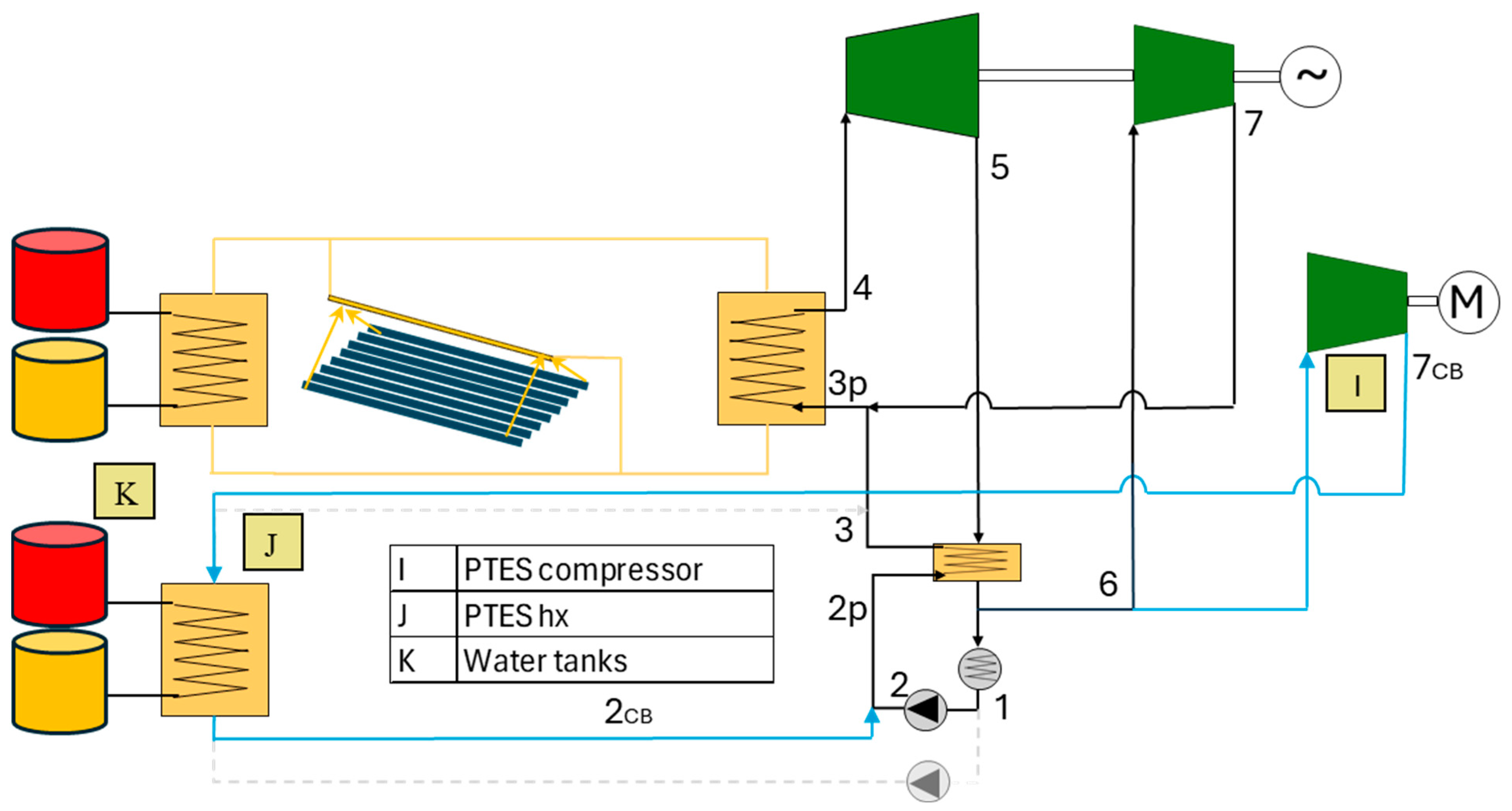
The layout of the HRB-PTES-propane at the charging process is shown in Figure 3. It includes the following new components that are added to the system: the two water tanks for the PTES storage system, the water–propane heat exchanger (PTES HX), and the PTES compressor for the heat upgrade to charge the PTES.

Table 3. Summarized HRB-CB-propane data input.

T8 (°C)	47.3
Propane compressor fraction	0.25
Water/propane HX PP (°C)	5
Cold water tank temperature (°C)	42.3
Storage capacity (hours)	3–4

summarizes its data. Three and four hours of storage are considered in the analysis.

During charging, water is taken from the cold tank, heated up with the propane fraction coming from the additional compressor, and finally introduced to the hot tank. The additional fraction of propane is taken from the low-pressure side of the recuperator, which is subtracted from the main fraction that goes to the condenser and is directed to the second compressor instead. The PTES compressor is identical to that of the reference configuration, but it runs on a separate shaft. Under nominal conditions, the PTES compressor rotates at the same speed as the reference one, so the flow rate and thermodynamic conditions for both configurations coincide. Furthermore, under nominal conditions, the thermodynamic state of the propane at the outlet of the storage system is the same as that of the main stream after the pump. The rest of the thermodynamic states coincide with those of a reference plant. A pinch point of 5 °C is considered in the water/propane heat exchanger. The water pump operates at a constant flow rate.

Figure 4 shows the T-s diagram of the charging layout under nominal conditions, where the equality of the properties of the states mentioned earlier can be observed.

Under off-design conditions, the PTES compressor speed is controlled to maintain the same mass flow rate as at nominal conditions, which provides certain advantages compared with the case of being the same as that of the turbine shaft. If the compressor were on the same shaft as the turbine, the propane mass flow rate passing through it would depend on the ambient temperature, since the pressure at the compressor inlet coincides with the condensation pressure. At ambient temperatures higher than the nominal value, the value of both the propane mass flow rate and the temperature at the compressor outlet would increase, as the temperature at the compressor inlet would also be higher. This would cause the water–propane heat exchanger to be unbalanced and lead to excessive compressor consumption work and excessively high temperatures in the hot tank. Furthermore, this would result in higher costs for the water tanks because of the increased pressure they should guarantee. These issues are avoided by keeping constant the propane mass flow rate that passes through the compressor.

The layout of the HRB-PTES-propane at the discharging process, including also the second pump to circulate propane, is shown in Figure 5. In this operation mode, both compressors are turned off, and the bypassed mass flow required to balance the recuperator (balancing flow) comes from the new pump, and it is now heated with the thermal energy previously stored in the water tanks. The use of a pump instead of a compressor reduces the energy consumption, increasing the gross power rate compared with the reference configuration and restoring the electricity that was consumed by the new compressor during the charging mode.

The introduction of the PTES also improves the off-design behaviour of the system over the reference one since a more constant bypass flow rate is achieved when the condensation pressure varies, resulting in a more balanced recuperator and higher overall efficiency than in the original configuration.

Finally, when the PTES is deactivated (it neither charges nor discharges), the HRB-PTES-propane behaves like the reference CSP case.

4. Methodology

4.1. Component Design and Sizing

4.1.1. PTES Compressor

The polytropic efficiency is used to calculate the inlet and outlet states related to the turbomachinery. To account for polytropic efficiency in a discretized way, the total enthalpy variation in each turbomachinery is divided into 25 parts. For the compressor, Equation (1) is used to calculate every step of the compression process.

$${\eta }_{\mathrm{c}\mathrm{o}\mathrm{m}\mathrm{p}}=\frac{\delta h_s}{\delta h}$$

(1)

The thermodynamic states at the inlet and outlet of the compressor and its flow rate, along with the parameters from

Table 4. Nominal input parameters for the design of the compressor.

Degree of reaction (R)	0.5
Equivalent diffusion ratio (DRE)	1.95
Mean angle (βm)	45°
Mean diameter/height ratio (DmH)	2
Mach number (M)	<0.7

, are used to size the compressor, which is designed as an axial one. That design is required for the cost estimation of the equipment.

The material considered is stainless steel. A constant mean diameter is considered. At nominal conditions, the specific work is the same for all the stages of the compressor. R is fixed to 0.5, DRE is set to 1.95 to avoid boundary layer detachment in the blades [34] and β_m (mean angle of the flow direction) is set to 45° in order to maximize efficiency [34]. The maximum allowed Mach number at the compressor inlet is 0.7. The solidity, pitch/height ratio, and number of stages are other parameters that must be adjusted. Once the inlet pitch/height ratio of the first rotor stage is selected, the others are calculated considering that the value of the pitch of the last stage is 60% of the initial one and that the pitch varies linearly for each stage. This approach avoids an excessive number of blades in the last stages compared with the first ones.

Profile losses are assessed considering Lieblein correlation. Annular and secondary losses are calculated using Howell correlations. The correlations and references used are shown in Appendix A.

4.1.2. Water/Propane Heat Exchanger

The specific heat of propane undergoes significant variations around the critical point, so considerable errors in the calculation of the UA factors can occur if the total enthalpy change is not divided into smaller segments in which the specific heat can be considered constant. The enthalpy change is divided into 25 parts. This number leads to temperature variations small enough for employing the arithmetic mean temperature difference instead of the logarithmic mean temperature difference in each segment without making noteworthy errors. The total UA factor is calculated as the sum of the UA of each one of the 25 parts in which it is divided (Equation (2)). The UA of each small part is calculated from the heat exchanged (${\dot{Q}}_j$) and the arithmetic mean temperature difference ${(\mathrm{A}\mathrm{M}\mathrm{T}\mathrm{D}}_j$).

$$UA={\sum }_{j=1}^{25}{UA}_j={\sum }_{i=1}^{25}\frac{{\dot{Q}}_j}{{\mathrm{A}\mathrm{M}\mathrm{T}\mathrm{D}}_j}$$

(2)

The heat exchanger is modelled as shell and tube type with single segmental and one pass per tube and shell. The material used is stainless steel. The heat exchanger has a special high-pressure closure and a fixed tubesheet, so it meets the TEMA “DEN” standard. The tube thickness is calculated considering the ASME code [35,36]. The sizing is performed for each one of the 25 parts.

Table 5. Input water/propane HX parameters.

External tube diameter (do)	$\left\{9.5; 12.5; 15.9\right\} (\mathrm{m}\mathrm{m})$
Pitch	$1.25d_o<p_{tb}<2d_o (\mathrm{m}\mathrm{m})$
Roughness	$0.02 (\mathrm{m}\mathrm{m})$
Tube thermal conductivity	50 $(\mathrm{W}/\mathrm{m}\mathrm{K})$
Baffle cut	$0.2{·D}_{Shell}$
Total shell pressure drop	<1.25 bar
Total length	<30 m
Length diameter ratio	$5<L/D_{Shell}<15$

shows the main input parameters. The baffle cut, roughness, and tube thermal conductivity are set to standardized values. The values of the inlet heat exchanger tube velocity, pitch, and external tube diameter are adjusted to meet the constraints of maximum pressure drop, total length, shell diameter, and total length-to-diameter ratio. These constrains take standard values and can be found in [23].

The sizing methodology for each part comprises several stages. First, the heat transfer coefficient in the tubes is assessed considering the Jackson correlation because it provides higher accuracy than the Dittus–Boelter one close to the critical point. The friction factor is calculated using Colebrook–White correlation. These correlations can be found in Appendix A. The Delaware method is used to calculate the shell heat transfer coefficient and pressure drop. This method is comprehensive and requires calculating numerous geometric variables of the heat exchanger. There are different versions of this method, and the one used here can be found in [37].

4.1.3. Pressurized Water Tanks

Cylindrical tanks are considered. Storage tanks are pressurized to avoid water boiling. Because there are both filled and empty tanks, the entire system must be pressurized (water and air) so all tanks must be interconnected at the top. A pressurization system ensures that the system pressure does not fall below the allowed limit value. Because of the high pressure of the system, the tanks have a high length-to-diameter ratio, so they are arranged horizontally. This avoids excessive hydrostatic pressures.

Each tank has one hour of storage capacity, so the total number of tanks required should be the number of storage hours plus one. For example, in the case of 3 h of storage, four tanks are needed, three of them full, and one empty, which will be charged while one of the others is discharged, and sequentially repeating the process. This reduces the number of tanks required compared with that required if we considered the same number of cold tanks as hot tanks.

The material considered is carbon steel SA-516 GR.70. The thickness considered is the maximum common commercially available value for steel plates, 50.8 mm. The diameter is calculated using Equation (3), where t stands for the thickness, P the internal pressure, and S is the allowable stress value from [35]. This expression is taken from [36]. Note than the pressure value is the vapour pressure value of the maximum water temperature expected during the simulation plus the hydrostatic pressure. Finally, the length of one tank is calculated to accommodate the volume of one hour of operation plus 5% of this value to assure a minimum level of water in the tank.

$$\mathrm{D}=\frac{2·\mathrm{t}}{\mathrm{e}\mathrm{x}\mathrm{p}\left(\raisebox{1ex}{$\mathrm{P}$}\!\left/ \!\raisebox{-1ex}{$\mathrm{S}$}\right.\right)-1}$$

(3)

The amount of insulation needed should be calculated to ensure that the maximum value of thermal losses under nominal conditions are 25 W/m². The material used is fiberglass wool. Different correlations have been considered to evaluate the external and internal film coefficients, depending on the type of surface. The curved internal surfaces of the cylinder are approximated to horizontal plates. Th corresponding to the lower half is considered an “upper surface of a cold plate” and the upper half a “lower surface of a cold plate”. The lateral closures are considered “vertical plates”. In Appendix A, the correlations are shown.

4.2. Off-Design Operation

The methodology for the off-design simulation of the systems assumes the following criteria:

(1)

The Stodola–Frügel Law is used to describe the behaviour of the turbine at part load [38].

(2)

The volumetric flow in the auxiliary compressor is considered constant.

(3)

The mass flow rate in the PTES compressor is considered constant.

(4)

The turbomachinery efficiency (of both compressor and turbine) varies at off-design conditions, and it is reduced from its nominal value as the capacity moves away from the design value according to Equation (4) [38]. Equation (5) describes the turbomachinery capacity from the mass flow rate, the inlet pressure, and the inlet temperature.

(5)

In the heat exchangers, the UA factors decrease as the mass flow rate of the fluid with the highest thermal resistance also does. The UA factor is calculated using Equation (6).

$${\eta }_{tb}={\eta }_{t{b}_{dis}}-\left|1-\frac{{\varphi }_{tb}}{{\varphi }_{t{b}_{dis}}}\right|/3$$

(4)

$$\varphi =\dot{m}\frac{\sqrt{T}}{P}$$

(5)

$${UA}_{obj}={UA}_{dis}·{\left(\frac{\dot{m}}{{\dot{m}}_{dis}}\right)}^{0.8}$$

(6)

4.3. Annual Simulations

4.3.1. Reference Configuration

The meteorological hourly data correspond to the typical meteorological year for Sevilla [39] and include the Direct Normal Irradiation and the dry bulb ambient temperature. The market hourly price data correspond to the year 2022, and they were obtained from [40].

The dispatch strategy of the TES of the reference CSP aims to supply energy around the electricity peak evening prices with only one start-up of the PB per day, as these are the hours with the highest average electricity selling prices. Production is scheduled during the 5-h period with the highest average monthly electricity prices, by default. This period is identified monthly. Daily, the period can be extended to adjacent hours as long as they have the next highest price. During the remaining hours, the PB is shut down, but the CSP can operate the solar field to store thermal energy in the TES. If the capacity of the salt tanks is exceeded or if the energy lost due to collector defocusing exceeds 15%, the simulation is recalculated on the same day considering that the PB starts up at dawn. This ensures that the TES has enough energy for the PB to produce from the peak morning price hours to the peak evening price hours.

The PB is shut down by default at 00:00 since the average electricity prices continue to drop during the night. However, the shutdown time can be extended to prevent dumping during the following day. The dispatch strategy is explained in detail in [41]. This reference also justifies the chosen values for production periods and the set limit for energy loss due to collector defocusing. Additionally, even though the years considered in [41] and in this paper are different, the strategy remains valid because the monthly hourly price values show similar trends. Figure 6 shows the hourly average electricity prices for each month for the year 2022.

The following operation conditions are considered:

(1)

The values of the HTF mass flow rate through the primary heat exchanger and the outlet temperature of the solar field always take the nominal value.

(2)

Ambient temperature and inlet SSG temperature at the HTF side (in the case that the TES transfers thermal energy to the PB) take off-design values.

(3)

The condensing temperature is set to 10 °C above the ambient temperature.

The thermal energy required to start up the PB and solar field, shadowing factors, and TES thermal losses are also considered. The methodology used to account for these factors is also described in [41].

4.3.2. HRB-PTES-Propane Plant

For the HRB-PTES-propane configuration, the same considerations as the reference case are taken into account. The same TES dispatch schedule is considered for the CSP part of the plant, in order to show an effective comparison between both solutions. For the calculation of heat losses in the tanks that are filled or emptied during the time step of the simulation, it is considered that they are at half capacity throughout the entire hour. It is also assumed that the air contained in the tank is at the same temperature as the liquid.

The dispatch strategy for the PTES part of the plant is set for every single day. Different scenarios are considered as follows:

(1)

When the PB operates from dawn to dusk, the PTES charges during the cheapest price period until it is full and discharges during the highest price hours until completely discharged. Only one cycle of PTES charging and discharging per day is considered. If on the next day, the PB only operates during the sunset, the PTES will not charge on that day. Thus, the discharge hours can be distributed between the two days, according to the maximum electricity hourly prices.

(2)

When the PB operates only during sunset for two consecutive days, the system can charge for two hours on one day and discharge for two hours on the following day, as long as the price difference is greater than a fixed value, for example, 30 EUR/MWh.

4.4. Economic Analysis

4.4.1. Estimation of the Capital Expenditure of the Components

The equipment costs are estimated considering the correlations in [42,43,44,45]. It includes the water/propane heat exchangers, storage tanks, compressor, water and propane pumps, and their respective motors. Cost correlations are provided in Appendix B. Since each correlation has a different time reference, the prices are updated using the ratio between the chemical engineering plant cost index (CEPCI) value from the current year of study and that of each reference. The costs obtained from the correlations are in USD, so a conversion rate of 0.95 EUR/USD is used.

4.4.2. Figures of Merit

As it was mentioned in the Introduction, several economic analyses are applied to the proposed system in order to assess its feasibility in different scenarios as well as to compare its performance to that obtained by other CB systems. For that, different figures of merits are required.

To analyse the feasibility of the PTES integration, two ratios are used. The cost–income ratio ($r_{CI})$ of a plant, used, for example, in [30], is the sum of the levelized cost of investment (LC_INV) and operation and maintenance (LC_O&M) divided by the levelized income (LI) (Equation (7)). It provides a figure to quantify if a system is feasible or not. Specifically, if $r_{CI}=1$, only the initial value of the investment is recovered at the end of the economic life of the plant, so no profit is obtained. On the contrary, when $r_{CI}$ is higher or lower than 1, it means the project is non-profitable or profitable, respectively. It should be noted that the considered costs and incomes are the incremental values of the HRB-PTES-propane case over the reference HRB-propane one. The economic scenario used is shown in

Table 6. Economic scenario.

$\mathrm{Yearly}\mathrm{O}\&\mathrm{M}\mathrm{equipment}\cos \mathrm{t}\mathrm{percentage}\mathrm{of}\mathrm{inversion}(C_{O\&M})$	$1\%·Inv$
Interest rate (r)	4%
Inflation (inf)	3.6%
Amortization years (N)	35

. It is considered that O&M and prices rise yearly according to the inflation rate. Appendix B shows the expressions used to calculate each levelized parameter.

$$r_{CI}=\frac{{LC}_{INV}+{LC}_{O\&M}}{LI}$$

(7)

In addition, the profit to income ratio ($r_{PI})$ is assessed using Equation (8) and, when it is positive, it represents the fraction of the income that is recovered as profits.

$$r_{PI}=\frac{{LI-(LC}_{INV}+{LC}_{O\&M})}{LI}$$

(8)

Finally, the LCOS, defined in Equation (9), is used to compare the obtained results to those reported for other proposals. $E_{in}$ stands for the annual energy that the CSP does not produce because of charging the PTES. It is calculated hourly, by subtracting the energy dispatched by the HRB-PTES-propane plant from that produced by the CSP when the PTES is off. $E_{out}$ is analogously calculated but considering the energy surplus of the HRB-PTES-propane plant when the PTES is discharging. Finally, $c_{el}$ is an average charging hourly price. This expression was obtained from references such as [30,46] but also considering inflation, like [47] does with the LCOE.

$$LCOS=\frac{{LC}_{INV}+{LC}_{O\&M}+E_{in}·c_{el}}{E_{out}}$$

(9)

In this work, in addition to calculating the LCOS for the specified economic and market scenario, the LCOS is compared with that calculated in other works. Specifically, the LCOS is compared with that calculated by [30] for various storage systems. As commented in the Introduction, that work considers the dispatch optimization of a storage system with a similar total capacity (4 h) during a specific market price year (Italy in 2019). The work also considers standardized electricity purchase prices. To enable comparison, the same economic scenario and standardized reference purchase price must be used. Furthermore, it must be verified that the strategy for dispatching energy does not vary to a large extent so that the LCOS remains constant regardless of the market price and the year (i.e., the price of the purchased electricity is fixed, and the yearly yield of the plant does not vary). To verify this, the schedule for dispatching is recalculated considering the hourly price market of the year 2019, and the LCOS is compared to that of the original year (2022) considering the same purchase price. If the LCOS remains constant, then the variation due to the selection of the dispatch strategy is not significant and the comparison with the LCOS of reference [30] can be considered valid.

A sensitive analysis of the cost, selling price, and financing scenario is also carried out. These analyses are performed separately in order to find the most influential parameter. In addition, as the cost correlations are subject to an inherent uncertainty, a comprehensive range for them (from −30% to +30% over the selected references) is considered. For the selling price sensitivity analysis, the electricity prices are varied, changing from the values from 2022 to 2019 (significantly different). Thus, the schedule for dispatching and the figures of merit are recalculated considering the electricity hourly market prices of the year 2019. For the financing sensitivity analysis, the same average scenario used in reference [30] is used. These data are shown in

Table 7. Average economic scenario of [30].

$\mathrm{Yearly}\mathrm{O}\&\mathrm{M}\mathrm{equipment}\cos \mathrm{t}\mathrm{percentage}\mathrm{of}\mathrm{inversion}(C_{O\&M})$	$3\mathrm{\%}·Inv$
Interest rate (r)	7%
Inflation (inf)	0
Amortization years (N)	30

.

5. Results

In Section 5.1, the results of sizing each component of the PTES are presented, which is required to estimate their costs. In Section 5.2, the behaviour of the CSP including the charging and discharging modes of operation of the PTES at different conditions is presented with the aim of showing the advantages of integrating the PTES within a CSP plant. Section 5.3 analyses the economic results of the base case and the scenarios proposed in the sensitivity analysis. Finally, in Section 5.4, the LCOS is calculated to compare the proposed system to other proposals using the same reference framework.

5.1. Sizing Results

The main results of the sizing of the propane–water heat exchanger, the water storage tanks, the propane compressor, and the equivalent air compressor are shown, respectively, in

Table 8. Water/propane heat exchangers summary data.

Total exchange area (m2)	11,026
Number of Hx	2
Layout	two in series
Summary results per HX
Area (m2)	5513
Internal tube pressure (bar)	170.5
Overall heat transfer coefficient (W/m2K)	781
Tube heat transfer coefficient (W/m2K)	1195
Shell heat transfer coefficient (W/m2K)	7854
Tube pressure drop (kPa)	20
Shell pressure drop (kPa)	115
Length (m)	16
Shell diameter (m)	1.69
Distance between baffles (mm)	540
Outlet tube diameter (mm)	12.5
Tube pitch (mm)	15.7
Tube thickness (mm)	1.2
Number of tubes	8739

,

Table 9. Water tank summary data.

	3 h Case	4 h Case
Total weight (t)	465.96	582.45
Number of tanks	4	5
Summary results per tank
Mass (t)	116.49
Length (m)	15
Diameter (m)	6.21
Thickness (mm)	50.8
Isolating thickness (mm)	236
Pressure (bar)	23.8
Hot tank nominal temperature (°C)	194.5
Nominal temperature drop per hour (°C)	0.038
Nominal thermal losses (kW)	8.5

and

Table 10. Propane compressor and air equivalent compressor summary data.

	Propane Compressor		Air Compressor
	First Rotor Stage	Last Rotor Stage	First Rotor Stage	Last Rotor Stage
Inlet pressure (bar)	12.2	136.2	1	8.7
Inlet temperature (°C)	53.6	189.2	28.5	315.87
Mean height (mm)	101.4	8.7	101.4	21.4
Pitch/height ratio	0.2	1.35	0.2	1.35
Pressure ratio	14		10.14
Shaft speed (rpm)	15,830		23,795
Mass flow (kg/s)	140.45		10.35
Total–total efficiency (%)	88.24		87.02
Flow coefficient	0.5
Load coefficient	0.454
Reaction grade	0.5
Number of stages	10
Mean diameter (mm)	215.8
Maximum Mach	0.69

.

The propane–water heat exchanger is divided into two heat exchangers in series to avoid excessive tube lengths. The area of each one along with the internal pressure of the tubes is used to calculate the costs.

The dimensions of the tanks are the same for both the 3-h and 4-h cases. The only difference is that five tanks are required for the 4-h case, whereas four tanks are required for the 3-h case. The weight of each tank is the parameter used to calculate the costs. The nominal temperature drop per hour refers to a hot-filled tank at the nominal temperature. Typically, hot-filled tanks are emptied before 24 h. In cases where the hot-filled tank remains full for 24 h, the approximate temperature loss is only 1 °C.

Table 10 shows the main results of the propane compressor, as well as those of an equivalent air compressor of the same size and stages as the propane one. The reason for this is that an air compressor correlation is used for cost estimation, so the mass flow rate, efficiency, and pressure ratio of the equivalent air compressor are the parameters required to calculate the equipment cost. For each compressor, the parameters at the first and last rotor inlet are shown. The total–total efficiency of the propane compressor corresponds to the isentropic efficiency calculated through the thermodynamic states at the inlet and outlet of the compressor. The maximum Mach is achieved at the inlet of the first rotor stage.

For the sizing of the equivalent air compressor, it is considered that both the flow coefficient, the loading coefficient, the degree of reaction, the number of stages, the Mach number at the inlet of the first rotor stage, solidity, as well as the pitch/height ratio of each stage are the same as those of the design propane compressor. The chosen inlet pressure is the ambient inlet pressure, as it is the most common in air compressors. The inlet air temperature, as well as the air mass flow rate, are the parameters that are adjusted to obtain the same mean diameter and the same mean blade height in the first rotor stage as those achieved in the propane compressor. It should be noted, however, that the height of the last stage differs between both compressors. This is because each fluid has unique characteristics, resulting in different compression processes. On the other hand, a significant disparity in flow rates between both compressors can be observed. This is primarily due to the difference in inlet density. Thus, for a given size of equivalent air compressor, the propane compressor consumes a considerably higher power.

The equipment costs including installation costs, for the 3-h and 4-h HRB-PTES-propane cases are shown in

Table 11. Equipment costs for the 3-h and 4-h HRB-PTES cases.

	Cost per Unit (M EUR/Unit)	Units		Total Cost (M EUR)
Compressor motor	1.153	1		1.153
Propane pump motor	0.496	1		0.496
Water pump motor	0.004	1		0.004
Compressor	3.04	1		3.04
Propane pump	1.995	1		1.995
Water pump	0.027	1		0.027
Heat exchanger	1.346	2		2.691
Tank	1.369	4	5	5.476	6.845
				14.882	16.251

. The water pump and its respective motor consumptions are negligible because of the low water flow rate and the low pressure drop in the propane–water heat exchanger. The costs of the pump and compressor motors are calculated assuming that the electric motors have an efficiency of 99%. The cost of the additional propane required is less than 0.1% of the total additional investment, so it is taken into account. It is assumed that the total volume occupied by the additional propane is twice the volume occupied by the propane in the water/propane heat exchangers.

5.2. Operation of HRB-PTES-Propane

Table 12. Main HRB-PTES operation results at nominal conditions (reference and charging).

	Reference	Charging
Condensing temperature (°C)	35	35
Cold storage temperature (°C)	-	42.3
Hot storage temperature (°C)	-	194.5
PB thermal power inlet (MW)	250.3	250.3
Thermal power evacuated through the condenser (MW)	150.2	100.1
Thermal power absorbed by PTES storage (MW)	-	65.4
Gross power produced (MW)	100	84.7
Net power consumption (MW)	93.3	80.1
Total propane mass flow (kg/s)	561.8	561.8
Auxiliary compressor consumption (MW)	20.4	20.4
PTES compressor consumption (MW)	-	20.4
Main pump consumption (MW)	15.1	10.1

compares the main results of the CSP when the PTES is off versus when it is charging under nominal conditions.

Table 13. Propane mass flow fraction through each component (reference and charging).

	Reference	Charging
Main pump	0.75	0.5
Recuperator high-pressure path	0.75	0.75
SSG	1	1
Turbine	1	1
Recuperator low-pressure path	1	1
Auxiliary compressor	0.25	0.25
PTES compressor	-	0.25
Condenser	0.75	0.5

shows the mass flow fractions circulating through each component for each case. These fractions are expressed as a fraction over the total propane mass flow rate.

During the charging, the evacuated thermal power is lower than in the reference case because the fraction of propane flow circulating through the condenser is also lower. This is due to the additional extraction passing through the PTES compressor. Furthermore, the difference in gross power produced is equal to the consumption of the PTES compressor minus the difference between the main pump consumptions for the two cases. The main pump consumption is different because it drives different flow fractions for each case.

Furthermore, it can be observed that the thermal power absorbed by the PTES storage is greater than the consumption of the PTES compressor. This is because the energy related to the enthalpy difference between the compressor inlet and the PTES storage outlet is also stored. This is shown in Equations (10) and (11). The nomenclature used is the same as that shown in Figure 3 and Figure 4. ${\dot{Q}}_{PTES}$ is the thermal power absorbed by the PTES storage, ${\dot{m}}_{prop-PTES}$ is the propane mass flow that goes through the PTES in the charging process, ${(h}_{7CB}-h_{2CB})$ is the specific enthalpy difference between the PTES storage inlet and outlet, ${(h}_{7CB}-h_6)$ is the specific enthalpy transferred from the compressor to the power fluid, and ${(h}_6-h_{2CB})$ is the specific enthalpy difference between the compressor inlet and PTES storage outlet. ${(h}_6-h_{2CB})$ can be evaluated considering sensible and latent energy contributions through Equation (12). $(h_6{-h}_{1v})$ and $(h_{1v}{-h}_{1l})$ refer to the equivalent sensible and latent energy that would be evacuated through the cooler. $h_{2CB}{-h}_{1l}$ is the specific enthalpy difference between the PTES storage outlet and the condenser outlet. If the energy stored related to the term ${(h}_6-h_{2CB})$ is not completely evacuated through the cooler during discharge, the overall efficiency of a PTES charging and discharging cycle will be higher than that obtained if the CSP had operated with the PTES off. This happens when the equivalent thermal energy that would be evacuated through the cooler in the reference case is stored in the charge and used later to produce power during discharge.

$${\dot{Q}}_{PTES}={\dot{m}}_{prop-PTES}·(h_{7CB}-h_{2CB})$$

(10)

$$h_{7CB}-h_{2CB}={(h}_{7CB}-h_6)+(h_6-h_{2CB})$$

(11)

$$(h_6-h_{2CB})=(h_6{-h}_{1v})+(h_{1v}{-h}_{1l})-(h_{2CB}{-h}_{1l})$$

(12)

Table 14. Main HRB-PTES operation results for a condensation temperature of 45 °C.

	Reference	Charge	Discharge
Condensing temperature (°C)	45	45	45
Cold storage temperature (°C)	0	70	70
Hot storage temperature (°C)	0	210.5	210.5
Bypassed propane maximum temperature (°C)	210.6	214.8	202.9
Outlet recuperator low-pressure side temperature (°C)	75	79	65.3
Inlet recuperator high-pressure side temperature (°C)	58.8	65.3	58.7
Recuperator heat capacity ratio (low pressure/high pressure)	1.08	1.06	0.99
PB thermal power inlet (MW)	236.7	235	240.3
Thermal power evacuated through the condenser (MW)	148.3	101.5	195.5
Thermal power absorbed by CB (MW)	-	61.0	−61
Gross power produced (MW)	88.4	72.5	105.7
Net power produced (MW)	82	67.8	96.4
Total propane mass flow (kg/s)	574.6	576.3	571.1
Auxiliary compressor consumption (MW)	24.2	24.6	-
PTES compressor consumption (MW)	-	21.1	-
Main pump consumption (MW)	15.2	10.2	16.1
PTES pump consumption (MW)	-	-	5
Power gross efficiency (%)	37.35	37.49
Efficiency difference (%)	0.14

compares the main results of the CSP when the PTES is off versus when the PTES is charging and discharging for a condensation temperature 10 °C higher than the nominal value.

Table 15. Propane mass flow fraction through each component for a condensation temperature of 45 °C.

	Reference	Charge	Discharge
Main pump	0.71	0.46	0.76
PTES pump	-	-	0.24
Recuperator high-pressure path	0.71	0.71	0.76
SSG	1	1	1
Turbine	1	1	1
Recuperator low-pressure path	1	1	1
Auxiliary compressor	0.29	0.29	-
PTES compressor	-	0.24	-
Condenser	0.71	0.46	1

shows the mass flow fractions circulating through each component for each case. The bypassed propane high temperature stands for the temperature reached by the propane at the outlet of the auxiliary compressor for either the reference case or at the PTES compressor outlet when charging. In the discharge case, the bypassed propane high temperature stands for the propane temperature at the outlet of the PTES storage. The difference between the temperature of the hot tank and the bypassed propane maximum temperature is due to irreversibility in the heat transfer in the propane/water heat exchanger. The chosen cold-water temperature for the charging case is the one that allows for obtaining the same value of cold-water temperature during discharge. In this way, the heat absorbed and evacuated by the PTES storage coincide, and the power gross efficiency obtained in the reference case can be compared to the power gross efficiency of a PTES operational cycle.

It should be noted the gross power efficiency does not consider the consumption of the fans of the air condenser. It can be observed that the power gross efficiency obtained for the PTES operational cycle is higher than that of the reference case. Since the condensing temperature (in this specific analysis) is the same in the charging and discharging process, the performance is increased solely because of the difference in sensible heat. A sign of this is that during discharge, the temperature at the outlet of the low-pressure side recuperator is lower than in both the charging and reference cases. This means that the sensible heat transferred to the cooler during discharging is lower than in the reference case.

The reason for the decrease in outlet temperature from the low-pressure side of the recuperator is that the recuperator is better balanced during discharge. This means that the heat capacity ratio between both low- and high-pressure flows is closer to one, compared with the reference case. The heat capacity ratio is defined in Equation (13). In the reference case, since the auxiliary compressor is coupled to the turbine, an excessive fraction of propane is bypassed. As a result, the thermal capacity of the fluid on the low-pressure side of the recuperator becomes greater than that on the high-pressure side. This leads to a higher outlet temperature for the propane on the low-pressure side. However, during PTES discharge, the bypass fraction flow is controlled by a pump. As a result, the thermal capacities of both fluids in the recuperator are balanced, leading to a lower outlet temperature of the recuperator on the low-pressure side.

$$\frac{{\dot{m}}_{low}·c_{p-low}}{{\dot{m}}_{high}·c_{p-high}}=\frac{∆T_{high}}{∆T_{low}}$$

(13)

Table 16. Main HRB-PTES operation results for a condensation temperature of 25 °C.

	Reference	Charge	Discharge
Condensing temperature (°C)	25	25	25
Cold storage temperature (°C)	-	47	46.9
Hot storage temperature (°C)	-	194.8	195.0
Propane bypass high temperature (°C)	194.4	199.2	184.1
Outlet recuperator high-pressure side temperature (°C)	37.9	42.9	42.1
Inlet recuperator high-pressure side temperature (°C)	36.0	41.5	36.1
Recuperator heat capacity ratio (low pressure/high pressure)	0.9	0.92	1
PB thermal power inlet (MW)	267.6	267	264.4
Thermal power evacuated through the condenser (MW)	157	110.4	203.4
Thermal power absorbed by CB (MW)	-	63.6	63.7
Gross power produced (MW)	110.6	92.9	124.7
Net power produced (MW)	103.5	88	115.3
Total propane mass flow (kg/s)	547.4	547.9	549.9
Auxiliary compressor consumption (MW)	17.3	17.5	-
PTES compressor consumption (MW)	-	22.4	-
Main pump consumption (MW)	15	10.3	14.1
PTES pump consumption (MW)	25	-	5
Power gross efficiency (%)	41.33	40.95
Efficiency difference (%)	−0.38

compares the main results of the CSP when the PTES is off versus when the PTES is charging and discharging for a condensation temperature 10 °C lower than the nominal value.

Table 17. Propane mass flow fraction through each component for a condensation temperature of 25 °C.

	Reference	Charge	Discharge
Main pump	0.79	0.54	0.74
PTES pump	-	-	0.26
Recuperator high-pressure path	0.79	0.8	0.74
SSG	1	1	1
Turbine	1	1	1
Recuperator low-pressure path	1	1	1
Auxiliary compressor	0.21	0.26	-
PTES compressor	-	0.29	-
Condenser	0.79	0.54	1

shows the mass flow fractions circulating through each component for each case.

In this new analysis, the efficiency of the plant with the integrated PTES is lower than that of the reference plant. It can be observed that, unlike the previous case, the temperature at the outlet of the low-pressure side recuperator is higher during discharge than the temperature reached when the PTES is off. In contrast to the previous case, the heat capacity is lower than one. This happens because as the inlet pressure of the auxiliary compressor is lower than nominal, a smaller fraction than necessary to balance the thermal capacities of both fluids is diverted. However, unlike in the previous case, the work of the auxiliary compressor is also lower, so the efficiency in the reference is reduced less.

It should be noted that, in most cases, charging and discharging do not occur at the same temperature. Charging typically occurs at a higher temperature, while discharging occurs at a lower temperature. Electricity prices tend to be cheaper during the warmer hours of the day and more expensive in the evening. The efficiency in this case is improved because the maximum temperature reached by the bypassed propane during the PTES discharge is higher than if the charging were performed at a lower condensing temperature. On the other hand, both charging and discharging typically occur at ambient temperatures higher than the nominal temperature. This is because the CSP operates for a greater number of hours during the summer months. As demonstrated previously, this has positive effects on efficiency, contributing to the introduction of synergies.

5.3. Annual Results and Sensitivity Analysis

Table 18. Annual economic results for the reference case and the 3 h and 4 h HRB-PTES cases.

	Reference Case	3 h HRB-PTES	4 h HRB-PTES
Net energy (GWh)	331.26	331.3	331.3
CSP capacity factor (%)	41.7	41.7	41.7
PTES capacity factor (%)	-	13.5	17.49
Income (M EUR)	57.41	58	58.11
Incremental income (M EUR)	-	0.59	0.7
Incremental inversion (M EUR)	-	14.88	16.25
Cost–income ratio	-	1.01	0.94
Profit–income ratio (%)	-	−1.53	5.46
Charging electricity price (EUR/MWh)	-	137.4	139.2
Discharging electricity price (EUR/MWh)	-	206.7	202.9

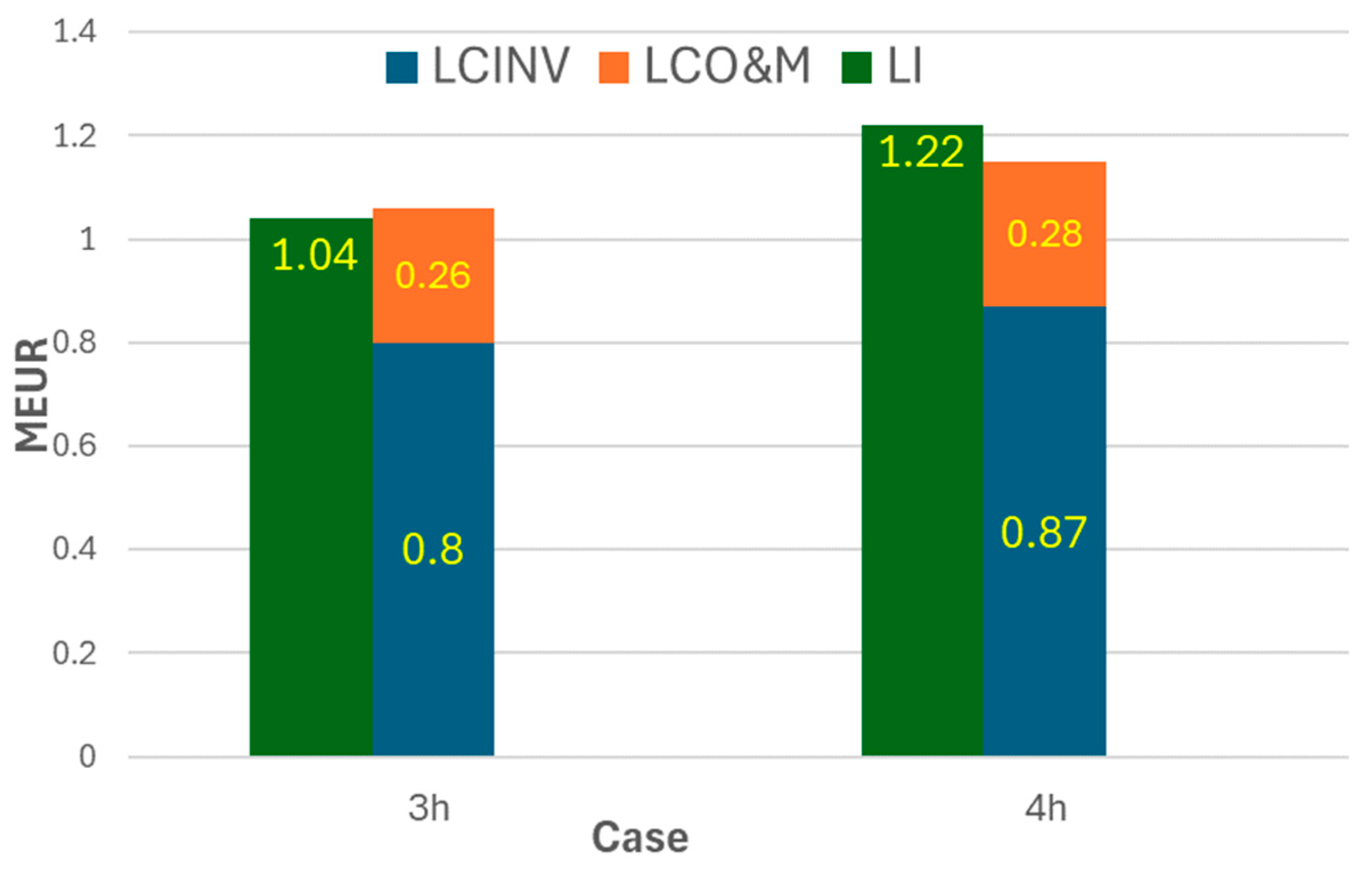
shows the annual economic results for the reference case, the HRB-PTES-propane with 3 h of storage, and the HRB-PTES-propane with 4 h of storage. Figure 7 shows the values of LC_INV, LC_O&M, and LI for the two cases presented in Table 18. If LI is greater than the sum of LC_INV and LC_O&M, the project is profitable. This agrees with the values of the figures of merit in Table 18. The net energy of the HRB-PTES-propane cases is slightly higher than that of the reference case. This is due, in part, to the synergies explained in the previous section about the potential improvement in the PTES integration.

The capacity factor is the total number of operating hours of the CSP divided by the total hours of one year, while the PTES capacity factor considers the total number of operating hours of the PTES (charging plus discharging). The incremental incomes are calculated by subtracting the incomes of HRB-PTES-propane cases from the incomes of the reference case. The incremental investment refers to the total PTES equipment costs shown in Table 11 of Section 5.1. The 4-h HRB-PTES is feasible under the proposed economic scenario, offering 5.46% in the profit–income ratio. The 3-h HRB-PTES is not profitable as the cost–income ratio exceeds 1. The charging and discharging electricity prices refer to the average prices obtained during the simulation. As one can expect, the price difference between charging and discharging for the 3-h case is greater than that for the 4-h case.

Table 19. Economic results for the sensitivity analysis.

Case	INV (M EUR)	CO&M (M EUR)	INC (M EUR)	${\mathit{r}}_{\mathit{C}\mathit{I}}$	${\mathit{r}}_{\mathit{P}\mathit{I}}$ (%)
Base	16.251	0.162	0.698	0.94	5.46
+30% equipment cost	21.126	0.211	0.698	1.23	−22.9
−30% equipment cost	11.376	0.114	0.698	0,66	33.82
2019 market scenario	12.377	0.123	0.063	8	−699
Economic scenario of [30]	16.251	0.487	0.698	2.57	−157.5

shows the economic results for the sensitivity analysis. Only the HRB-PTES-propane case with 4 h of storage is analysed. Figure 8 shows the values of LC_INV, LC_O&M, and LI for the sensitivity analysis cases presented in Table 19. The “base case” is the same as that shown in Table 18. The “+30% equipment cost” and “−30% equipment cost” scenarios increase and reduce the investment cost by 30%, respectively. The maintenance cost is also affected, varying proportionally with the investment cost. In the “2019 market scenario”, the simulation is performed considering the year 2019 instead of 2022. The costs are also updated considering the CEPCI ratio between 2019 and 2022. Finally, the last case considers the financial scenario of the article [30] (as commented in the Methodology Section).

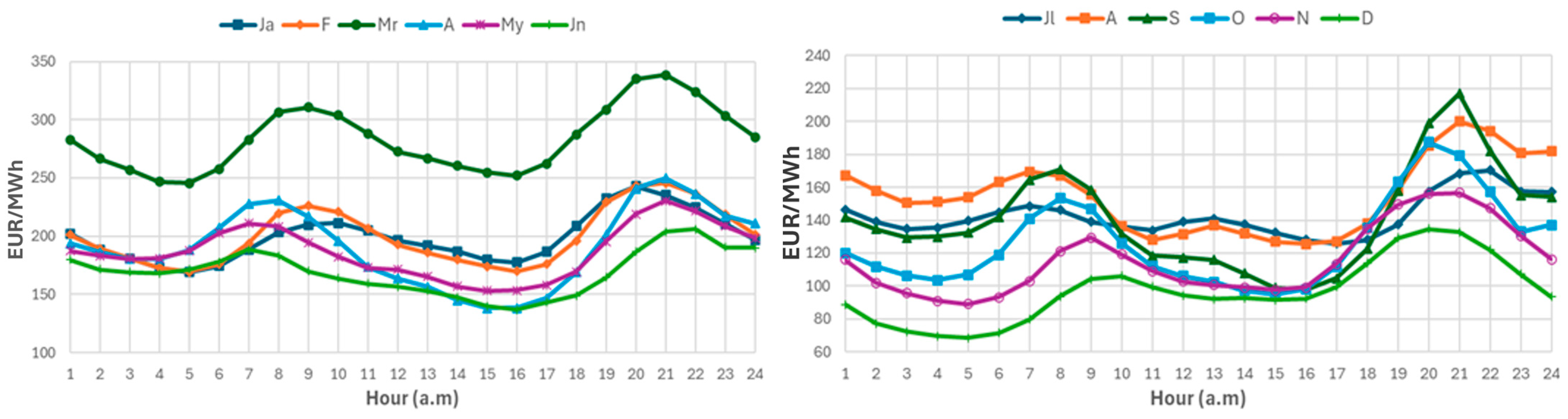
It can be observed that the feasibility is quite sensitive to the economic framework, concluding that, currently, incentives to systems aiming to stabilize the grid may be required. The worst scenario corresponds to the 2019 market scenario. It is observed that despite the lower investment cost compared with the base case, the levelized costs exceed the levelized revenues by 8 times. This is because the annual incomes are reduced almost tenfold compared with the base case. Next, a more detailed analysis is conducted on the differences in the electricity prices and incomes obtained for the years 2022 and 2019.

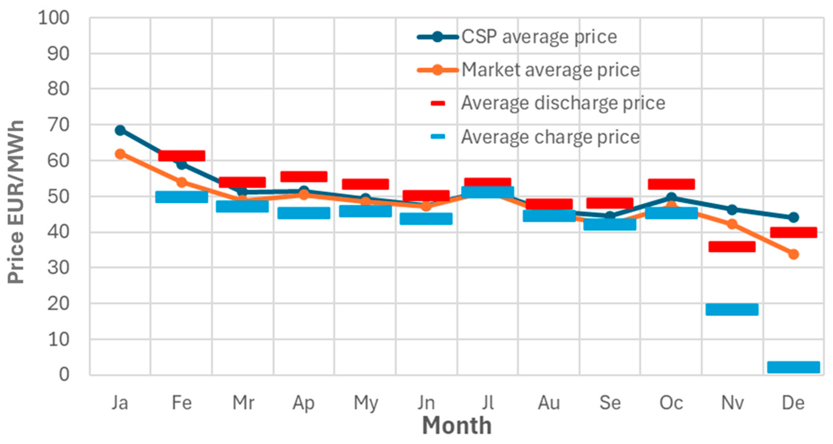
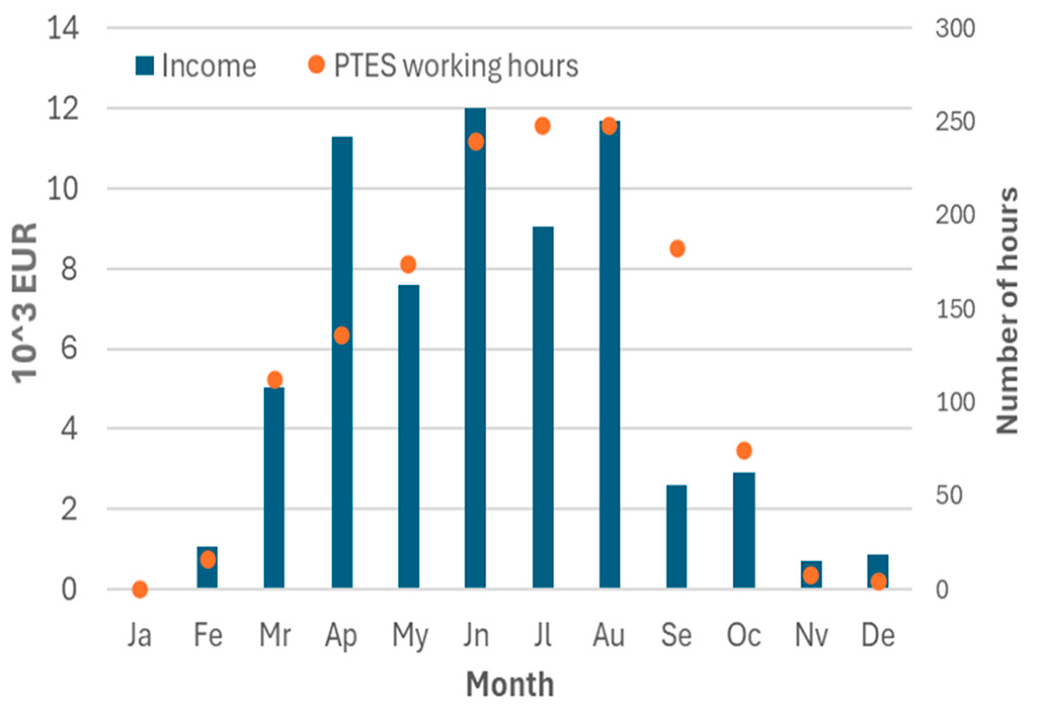
Figure 9 shows the monthly averages for 2022 of the CSP hourly price, market hourly price, PTES discharge hourly price, and PTES charge hourly price. Figure 10, respectively, shows the monthly incremental revenues and the number of monthly operational hours for the PTES. Figure 11 and Figure 12, respectively, show the same information as Figure 9 and Figure 10 but for the year 2019.

In Figure 9, it can be observed that the average price of the CSP tends to be higher than the market average during the months with lower radiation (January, February, March, October, November, and December). This is due to the dispatch optimization of the salt storage, which operates the PB preferably during the evening peak hours. In months with higher irradiation, as the operating hours of the CSP increase, the average price of the CSP tends to be the same as the average market price. It can also be observed that except for January, February, November, and December, the difference between the average discharge and charge electricity prices tends to be higher in months with lower irradiation and it tends to be lower in the summer. January, February, November, and December cannot be considered to follow this trend since the number of hours in which the PTES operates is not representative. In Figure 10, it can be observed that in months with higher radiation, the PTES operates for a greater number of hours, while in months with lower radiation, it operates for fewer hours. This is logical since the CSP operates for a larger time during months with higher radiation. Monthly revenues do not follow a clear trend because in months when the PTES typically operates for a few hours, the price difference tends to be high, and vice versa.

The average electricity prices in Figure 11 follow a similar trend as those in Figure 9; however, it can be observed that they are considerably lower. Also, it should be noted that during January, the PTES does not work. The reduction in the price difference between charging and discharging is significant. So, the monthly incomes are greatly reduced despite the number of working hours of the PTES being similar to those in the previous case. In Figure 13, the monthly revenues for the year 2022 and 2019 are presented. Finally,

Table 20. Summarized data of the 2022 and 2019 simulations.

	2022 Case	2019 Case
Market average price (EUR/MWh)	167.29	47.71
CSP average price (EUR/MWh)	180.82	93
Discharge average price (EUR/MWh)	203	51
Charge average price (EUR/MWh)	139	46
Incremental incomes (M EUR)	0.698	0.063
PTES number of working hours	1532	1449

summarizes the main annual results of the comparison between the two years.

5.4. Comparison of the Proposed PTES Integration to Those of Other Works

The sensitivity analysis conducted in the previous section revealed that, assuming the same economic scenario as [30], the cost-to-income ratio is 2.57. This is considerably lower (better) than the value obtained by [30] for the cheapest storage technology, which was 10. This suggests that, under the economic framework considered in this study, energy storage technologies seem to have higher profitability than in [30]. However, the frameworks are not the same and the feasibility of the proposed PTES cannot be directly compared. For this purpose, the LCOS is calculated using the same electricity purchase prices and financial scenario as in [30].

Table 21. PTES summary data.

	2022 Case	2019 Case
Input PTES gross power (GWh)	11.84	11.13
Output PTES gross power (GWh)	11.62	11.05
Input PTES net power (GWh)	10.17	9.42
Output PTES net power (GWh)	10.32	9.67
LCOS (EUR/MWh)	228.5	197.7

shows, respectively, the equivalent gross energy purchased (electricity not supplied to the grid and used to charge the PTES), the equivalent gross energy produced (compression work saved when discharging the PTES), the purchased net energy, and the equivalent net energy produced for the year 2022 and 2019. The difference between the net and gross energy is the consumption of the fans of the condenser.

Table 21 also shows the LCOS values obtained for the years 2022 and 2019 considering the net power values, a standardized purchase price of 50 EUR/MWh, and the financial scenario provided in [30]. The discrepancies between the LCOS of both years are due, on one hand, to the updating of equipment costs for each year, and, on the other hand, to the lower number of operating hours of the PTES in the year 2019 (because the price difference between peak and off-peak hours was sometimes very small).

For the comparison, the LCOS of the year 2022 is considered, as it is the most unfavourable. As it can be observed, the LCOS of the proposed integration is considerably lower than the average value reported in the reference [30] for Rankine and Brayton PTES (around 400 EUR/MWh). The obtained LCOS value is around the average value for a PHES (Pumped Hydro Energy Storage) with 4 h of storage according to [30], which is the cheapest technology.

6. Conclusions

In this work, an integrated PTES in a CSP operating with an HRB-propane power cycle has been proposed. This novel configuration allows for leveraging the dispatchability of CSP plants while introducing cost savings compared with conventional PTES, as it allows for the use of the same turbine as the reference power block. Additionally, the PTES storage takes advantage of synergies in performance that arise from charging the system at high ambient temperatures while discharging at low ambient temperatures. This allows, in some cases, for increasing the efficiency of the HRB-PTES-propane compared with the reference CSP configuration without the PTES integration.

The HRB-PTES-propane with 4 h of storage has proven to be feasible under the proposed economic scenario. However, it has been observed that the results are very sensitive to changes in the economic frame. The worst-case scenario is the simulation considering Spanish electricity market prices in 2019. In this scenario, the revenues are nearly 10 times lower than in the original one of 2022. This generates considerable uncertainty regarding the profitability of this type of technology, as there are only a few years between 2022 and 2019, while amortization periods tend to be longer (+30 years). Furthermore, this leads to the additional conclusion that incentives may be required to introduce systems that increase the dispatchability of renewable energy unless the market tends to high electricity price difference between peak and valley periods.

The LCOS of the proposed PTES has been compared to those of other studies using a common reference framework. The results demonstrate that the obtained LCOS is significantly lower (around 200 EUR/MWh less) than the average LCOS of other Brayton and Rankine PTES systems. Specifically, the obtained LCOS is similar to that of the cheapest storage technology, pumped hydro heat storage, which stressed the advantages of introducing the PTES within CSP plans instead of as a standalone plant. While more validation is needed through a comprehensive optimization, these results encourage further investigation into the project.

For future works, we recommend establishing an MILP (mixed-integer linear programming) model to optimize the production dispatch schedule of the PTES in order to maximize revenues. Similarly, the proposed PTES could be extended for integration into other power cycles that include a compression process, like the recompression sCO₂ cycles, where it can introduce similar benefits.

References

1. International Energy Agency. Renewables 2023. 2023. Available online: https://www.iea.org/reports/renewables-2023/electricity (accessed on 15 March 2024).
2. International Energy Agency. Grid-Scale Storage. Available online: https://www.iea.org/energy-system/electricity/grid-scale-storage (accessed on 15 March 2024).
3. International Energy Agency. Coal 2022. 2022. Available online: https://www.iea.org/reports/coal-2022/executive-summary (accessed on 15 March 2024).
4. REE. Non-Renewable-Electricity-Generation. Available online: https://www.sistemaelectrico-ree.es/en/spanish-electricity-system/generation/non-renewable-electricity-generation (accessed on 16 March 2024).
5. ENERSELVES. What Is the “Iberian Exception”? Available online: https://projects2014-2020.interregeurope.eu/enerselves/news/news-article/14992/what-is-the-iberian-exception/ (accessed on 16 March 2024).
6. Luo, X.; Wang, J.; Dooner, M.; Clarke, J. Overview of current development in electrical energy storage technologies and the application potential in power system operation. Appl. Energy 2015, 137, 511–536. [Google Scholar] [CrossRef]
7. Breeze, P. Chapter 3-Compressed Air Energy Storage. In Power System Energy Storage Technologies; Academic Press: Cambridge, MA, USA, 2018; pp. 23–31. [Google Scholar]
8. Liang, T.; Vecchi, A.; Knobloch, K.; Sciacovelli, A.; Engelbrecht, K.; Li, Y.; Ding, Y. Key components for Carnot Battery: Technology review, technical barriers and selection criteria. Renew. Sustain. Energy Rev. 2022, 163, 112478. [Google Scholar] [CrossRef]
9. Desrues, T.; Ruer, J.; Marty, P.; Fourmigué, J.F. A thermal energy storage process for large scale electric applications. Appl. Therm. Eng. 2010, 30, 425–432. [Google Scholar] [CrossRef]
10. McTigue, J.D.; White, A.J.; Markides, C.N. Parametric studies and optimisation of pumped thermal electricity storage. Appl. Energy 2015, 137, 800–811. [Google Scholar] [CrossRef]
11. Rabi, A.M.; Radulovic, J.; Buick, J.M. Pumped Thermal Energy Storage Technology (PTES): Review. Thermo 2023, 3, 396–411. [Google Scholar] [CrossRef]
12. Laughlin, R.B. Pumped thermal grid storage with heat exchange. J. Renew. Sustain. Energy 2017, 9, 044103. [Google Scholar] [CrossRef]
13. Dumont, O.; Frate, G.F.; Pillai, A.; Lecompte, S.; De Paepe, M.; Lemort, V. Carnot battery technology: A state-of-the-art review. J. Energy Storage 2020, 32, 101756. [Google Scholar] [CrossRef]
14. Newcastle University. Hot Rock Solution to Grid-Scale Energy Storage. Available online: https://www.ncl.ac.uk/press/articles/archive/2017/11/isentropic/ (accessed on 15 April 2024).
15. Morandin, M.; Maréchal, F.; Mercangöz, M.; Buchter, F. Conceptual design of a thermo-electrical energy storage system based on heat integration of thermodynamic cycles—Part A: Methodology and base case. Energy 2012, 45, 375–385. [Google Scholar] [CrossRef]
16. Ayachi, F.; Tauveron, N.; Tartière, T.; Colasson, S.; Nguyen, D. Thermo-Electric Energy Storage involving CO2 transcritical cycles and ground heat storage. Appl. Therm. Eng. 2016, 108, 1418–1428. [Google Scholar] [CrossRef]
17. Shu, G.; Yu, Z.; Liu, P.; Xu, Z.; Sun, R. Potential of a thermofluidic feed pump on performance improvement of the dual-loop Rankine cycle using for engine waste heat recovery. Energy Convers. Manag. 2018, 171, 1150–1162. [Google Scholar] [CrossRef]
18. Frate, G.F.; Ferrari, L.; Desideri, U. Multi-Criteria Economic Analysis of a Pumped Thermal Electricity Storage (PTES) with Thermal Integration. Front. Energy Res. 2020, 8, 528376. [Google Scholar] [CrossRef]
19. Frate, G.F.; Antonelli, M.; Desideri, U. A novel Pumped Thermal Electricity Storage (PTES) system with thermal integration. Appl. Therm. Eng. 2017, 121, 1051–1058. [Google Scholar] [CrossRef]
20. Henchoz, S.; Buchter, F.; Favrat, D.; Morandin, M.; Mercangöz, M. Thermoeconomic analysis of a solar enhanced energy storage concept based on thermodynamic cycles. Energy 2012, 45, 358–365. [Google Scholar] [CrossRef]
21. Meli, P. Tale of Fire and Ice. MAN Energy Solutions. Available online: https://www.man-es.com/discover/a-tale-of-fire-and-ice (accessed on 16 April 2024).
22. Xue, X.J.; Zhao, Y.; Zhao, C.Y. Multi-criteria thermodynamic analysis of pumped-thermal electricity storage with thermal integration and application in electric peak shaving of coal-fired power plant. Energy Convers. Manag. 2022, 258, 115502. [Google Scholar] [CrossRef]
23. Yong, Q.; Jin, K.; Li, X.; Yang, R. Thermo-economic analysis for a novel grid-scale pumped thermal electricity storage system coupled with a coal-fired power plant. Energy 2023, 280, 128109. [Google Scholar] [CrossRef]
24. Basta, A.; Basta, V.; Spale, J.; Dlouhy, T.; Novotny, V. Conversion of combined heat and power coal-fired plants to Carnot batteries—Prospective sites for early grid-scale applications. J. Energy Storage 2022, 55, 105548. [Google Scholar] [CrossRef]
25. Yong, Q.; Tian, Y.; Qian, X.; Li, X. Retrofitting coal-fired power plants for grid energy storage by coupling with thermal energy storage. Appl. Therm. Eng. 2022, 215, 119048. [Google Scholar] [CrossRef]
26. Vecchi, A.; Knobloch, K.; Liang, T.; Kildahl, H.; Sciacovelli, A.; Engelbrecht, K.; Li, Y.; Ding, Y. Carnot Battery development: A review on system performance, applications and commercial state-of-the-art. J. Energy Storage 2022, 55, 105782. [Google Scholar] [CrossRef]
27. Smallbone, A.; Jülch, V.; Wardle, R.; Roskilly, A.P. Levelised Cost of Storage for Pumped Heat Energy Storage in comparison with other energy storage technologies. Energy Convers. Manag. 2017, 152, 221–228. [Google Scholar] [CrossRef]
28. McTigue, J.D.; Farres-Antunez, P.; J, K.S.; Markides, C.N.; White, A.J. Techno-economic analysis of recuperated Joule-Brayton pumped thermal energy storage. Energy Convers. Manag. 2022, 252, 115016. [Google Scholar] [CrossRef]
29. Risthaus, K.; Madlener, R. Economic Analysis of Electricity Storage Based on Heat Pumps and Thermal Storage Units in Large-Scale Thermal Power Plants. In Energy Procedia; Elsevier Ltd.: Amsterdam, The Netherlands, 2017; pp. 2816–2823. [Google Scholar] [CrossRef]
30. Frate, G.F.; Ferrari, L.; Desideri, U. Energy storage for grid-scale applications: Technology review and economic feasibility analysis. Renew. Energy 2021, 163, 1754–1772. [Google Scholar] [CrossRef]
31. Rovira, A.; Muñoz, M.; Sánchez, C.; Martínez-Val, J.M. Proposal and study of a balanced hybrid Rankine-Brayton cycle for low-to-moderate temperature solar power plants. Energy 2015, 89, 305–317. [Google Scholar] [CrossRef]
32. Muñoz, M.; Rovira, A.; Sánchez, C.; Montes, M.J. Off-design analysis of a Hybrid Rankine-Brayton cycle used as the power block of a solar thermal power plant. Energy 2017, 134, 369–381. [Google Scholar] [CrossRef]
33. Rovira, A.; Muñoz, M.; Sánchez, C.; Barbero, R. Advanced thermodynamic cycles for finite heat sources: Proposals for closed and open heat sources applications. Appl. Therm. Eng. 2020, 167, 114805. [Google Scholar] [CrossRef]
34. Muñoz, M.; De Antonio, A.R. Máquinas Térmicas; Universidad Nacional de Educación a Distancia: Madrid, Spain, 2016. [Google Scholar]
35. ASME-SECTION VIII DIVISION 2. Rules for Construction of Pressure Vessels. 2019. Available online: https://www.asme.org/shop/certification-accreditation (accessed on 15 September 2023).
36. ASME-SECTION II. Materials. Boiler and Pressure Vessel Code. 2019. Available online: https://www.asme.org/shop/certification-accreditation (accessed on 15 September 2023).
37. Serth, R.W. 6—The Delaware method. In Process Heat Transfer; Serth, R.W., Ed.; Academic Press: Cambridge, MA, USA, 2007; pp. 245–275. [Google Scholar]
38. Rovira, A.; Barbero, R.; Ortega, G.; Subires, A.; Muñoz, M. Towards High Solar Contribution in Hybrid CSP-Combined Cycle Gas Turbine Plants. Int. J. Energy Res. 2023, 2023, 8289873. [Google Scholar] [CrossRef]
39. METEONORM. Typical Meteorogical Year Datasheet. 2022. Available online: https://bigladdersoftware.com/epx/docs/8-3/auxiliary-programs/source-weather-data-formats.html#:~:text=The%20IWEC%20data%20files%20are,U%20S%20National%20Climatic%20Data%20Center (accessed on 16 March 2024).
40. OMIE. OMIE. Publications. Available online: https://www.omie.es/en/publications (accessed on 16 March 2024).
41. Subires, A.J.; Rovira, A. Economic Optimization of a Thermal Solar Power Plant That Operates with a HRB Cycle by Improving the Operation Schedule. SolarPACES Conf. Proc. 2023, 1. [Google Scholar] [CrossRef]
42. Bejan, A.; Tsatsaronis, G.; Michael, M. Thermal Design & Optimization; John Wiley & Sons: New York, NY, USA, 1996. [Google Scholar]
43. Turton, R.; Shaeiwitz, J.A.; Bhattacharyya, D.; Whiting, W.B. Analysis, Synthesis, and Design of Chemical Processes, 3rd ed.; Pearson Education: London, UK, 2009. [Google Scholar]
44. Towler, G.; Sinnott, R. Chemical Engineering Design Principles, Practice and Economics of Plant and Process Design; Butterworth-Heinemann: Oxford, UK, 2008; Available online: http://elsevier.com (accessed on 10 September 2023).
45. Shamoushaki, M.; Niknam, P.H.; Talluri, L.; Manfrida, G.; Fiaschi, D. Development of cost correlations for the economic assessment of power plant equipment. Energies 2021, 14, 2665. [Google Scholar] [CrossRef]
46. Jülch, V. Comparison of electricity storage options using levelized cost of storage (LCOS) method. Appl. Energy 2016, 183, 1594–1606. [Google Scholar] [CrossRef]
47. Montes, M.J.; Rovira, A.; Muñoz, M.; Martínez-Val, J.M. Performance analysis of an Integrated Solar Combined Cycle using Direct Steam Generation in parabolic trough collectors. Appl. Energy 2011, 88, 3228–3238. [Google Scholar] [CrossRef]
Figure 1. Reference configuration CSP layout.
Energies 17 02005 g001
Figure 2. HRB propane T-S diagram.
Energies 17 02005 g002
Figure 3. Charge process layout.
Energies 17 02005 g003
Figure 4. Charge process T-S diagram under nominal conditions.
Energies 17 02005 g004
Figure 5. Discharge process layout.
Energies 17 02005 g005
Figure 6. Hourly average electricity prices for each month for the year 2022. (left) First six months of 2022. (right) Last six months of 2022.
Energies 17 02005 g006
Figure 7. LCINV, LCO&M, and LI for the 3 h and 4 h HRB-PTES cases.
Energies 17 02005 g007
Figure 8. LCINV, LCO&M, and LI for the sensitivity analysis cases.
Energies 17 02005 g008
Figure 9. Average monthly electricity prices in 2022.
Energies 17 02005 g009
Figure 10. Monthly incomes and PTES working hours in 2022.
Energies 17 02005 g010
Figure 11. Average monthly electricity prices in 2019.
Energies 17 02005 g011
Figure 12. Monthly incomes and PTES working hours in 2019.
Energies 17 02005 g012
Figure 13. Monthly incomes comparison between 2022 and 2019.
Energies 17 02005 g013