Unit Commitment Considering Interruptible Load for Power System Operation with Wind Power

Abstract

A high wind-power penetration level causes increased uncertainty in power system operation because of the variability and limited predictability of wind generation. This paper proposes a novel type of unit commitment (UC) considering spinning reserve and interruptible load (IL) as operating reserve facilities to increase system flexibility for reliable, economical operation. Two uncertainty sources, load and wind generation, were modeled via autoregressive moving averages (ARMA). The formulation of interruptible load was considered in the implementation of unit commitments. Lagrangian relaxation-dynamic programming (LR-DP) was used to solve the unit commitment problem efficiently. The expected energy not supplied (EENS) was regarded as a probabilistic reliability criterion. The effectiveness of the proposed unit commitment was evaluated using an IEEE 118-bus system. The simulation results clearly demonstrated that with demand-side participation, the operating cost was significantly reduced when handling the increased uncertainty due to wind power integration within the required reliability criteria.

1. Introduction

As the proportion of wind energy in power systems increases, independent system operators (ISO) are becoming concerned with the challenge of how to operate their systems to cope with the resulting increased uncertainty. For stable system operation, a power balance must be maintained under all circumstances, and hence system operators must adjust the power output of dispatchable (controllable) generating resources to match the variations in the net demand. The increased uncertainty due to wind energy integration increases not only the operating cost of maintaining the short-term power balance, but also the frequency of short-term scarcity events caused by ramping capability shortages [1]. The key to solving this problem is generation flexibility, which depends on the generating resources (flexible resources, energy storage) and/or demand-side resources (DSR).

Traditionally, system operators exploit unit commitments (UC) to determine appropriate on/off states and dispatch for each generating unit to meet the predicted system load. UC is important optimization tasks in centralized power system operations in terms of system reliability and economics. The UC objective is to minimize the total operating cost of maintaining a power balance over a specific short-term period under given system and unit constraints, such as generator power output limits, system spinning reserve, ramp rate limits, and minimum up and down times of the units. Existing UC must be revised in order to accommodate wind power uncertainty, which makes power systems highly unpredictable and vulnerable. Numerous studies of wind power integration have been conducted to define, investigate, and understand these issues, and to find UC solutions. Various technical approaches have been devised to determine optimal generation scheduling in a wind-integrated power system at an allowable reliability level [2,3,4]. However, most of these techniques consider only generation, and exclude demand-side resources.

In this paper, we propose a novel approach to UC by considering interruptible load as an operating reserve, so that power system operations are robust against system uncertainties. Generally speaking, operating reserves are defined as any capacity available to assist in maintaining the active power balance, and are a necessity due to load forecasting errors, the unpredictable output of wind generation, and/or equipment failure. Since operating reserves comprise spinning and non-spinning reserves, only spinning reserves are considered in the short-term generation-scheduling problem [5]. An ISO can procure spinning reserves from both generating units and demand-side resources. Online units can provide spinning reserves to a system if they are not fully loaded and are ready to generate more power within an acceptable ramping capability. Loads that can be interrupted for a given time are also regarded as spinning reserves. An interruptible load is one with a prior customer agreement to reduce the load at peak demand times or at any time requested by the ISO. When customers sign an interruptible load contract, they are rewarded with capacity payment incentives, and they receive an additional reward for actual load reduction. Much has been written about interruptible load as a spinning reserve owing to the fact that it is much more economical to include demand-side reserves instead of only considering supply-side reserves [6]. However, spinning reserves obtained from generators can be expensive, since additional generating units are required, and the output of other units may be forced to deviate from the optimal point. Hence, operating costs increase significantly if power system operators provide spinning reserves only from dispatched generators. In light of the above considerations, it is quite reasonable to take demand-side participation into account, especially when there are increased operating reserve needs. Accordingly, in this paper, we assume that an ISO can procure spinning reserves from both generators and interruptible load.

Optimization techniques for efficiently solving UC problems are highly important since the problems are large scale and nonlinear. The solution procedure directly affects the convergence and computational time. Various mathematical programming methods and optimization techniques have been applied to UC problems, including priority-list, branch-and-bound, dynamic programming (DP), mixed-integer programming (MIP), and Lagrangian relaxation (LR) [7,8,9,10]. The priority-list method is fast, but the quality of the solution is too coarse for practical applications. Application of the branch-and-bound method is limited to small-scale power systems because of the dimensionality curse. Although DP is a flexible technique for solving UC problems, it may still give rise to high-dimensionality problems when applied to modern power systems due to the large number of generating units. The MIP method presents scalability drawbacks, and thus is a burdensome way of handling UC problems for large power systems [11]. On the other hand, the LR method provides a fast solution, and is the most efficient and realistic technique for large-scale problems. In the LR method, system constraints, rather than generating unit constraints, are relaxed by using Lagrangian multipliers corresponding to the load and spinning reserve requirements. A dynamic search is then performed at these stages using a DP solution to the UC combined with LR; i.e., LR-DP. This approach exploits the advantages of LR and DP in order to improve computational efficiency.

The remainder of this paper is organized as follows: Section 2 introduces probabilistic modeling of wind power and load evaluated via autoregressive moving averages (ARMA). Section 3 describes the conventional and proposed UC formulations. Techniques for solving the proposed UC formulation are provided in Section 4. Section 5 presents numerical results for the proposed method, and Section 6 summarizes our conclusions.

2. Wind Power and Load Modeling

For a given wind generation and load and probabilistic distribution function for forecasting errors, we considered both conventional and the proposed UC approaches, and then computed the expected operating cost considering uncertainties. Although the forecasted wind generation and load were treated as given in the UC problem, uncertainty modeling was needed when assessing the expected operating cost. In this paper, two types of uncertainty were considered: one related to the load and one related to the wind generation.

It is generally acknowledged that the wind speed in a given location closely follows a Weibull or Rayleigh distribution. However, generated wind speed using Weibull distribution may not properly reflect the correlation in the time domain [12], which may significantly affect UC result. ARMA model can take into consideration the characteristic that the wind speed at any time tends to be close to the immediately previous wind speed; in other words, there are no sudden changes in wind speed.

The general ARMA (p,q) model can be formulated as a model having an autoregressive order p and a moving average term q. We adopted ARMA (3,2) model to generate hourly wind speed in accordance with reference [13]. The authors established the ARMA (3,2) model after computing the actual hourly wind speed for three years and standard deviation of the wind speeds by the Least Squares method which minimizes the error terms. This model is given by:

V_t = δ + ϕ₁V_{t − 1} + ϕ₂V_{t − 2} + ϕ₃V_{t − 3} + e_t + θ₁e_{t − 1} + θ₂e_{t − 2}

(1)

We compute the active power of wind turbine with the following formula whose wind speeds V_t are generated by the above mentioned ARMA model. In order to derive wind power, additional information of air density (ρ), swept area of wind turbine (A), and power coefficient (C_p) are needed. Power coefficient C_p is affected by tip speed ratio and blade pitch angle where tip speed ratio is defined as blade tip speed divided wind speed [14]. For the sake of simplicity, we assumed the air density (ρ) and power coefficient (C_p) are 1.25 (kg/m³) and 0.446, respectively. The swept area of wind turbine is determined by the rotor diameter of wind turbine:

(2)

For the dynamic load L_t modeling, we use the following equation where FL_t is forecasted load and UL_t represents uncertainty in load:

L_t = FL_t + UL_t

(3)

Hourly forecasted load FL_t value is obtained from the IEEE 118-bus system. The deviation between actual load and forecasted load, namely uncertainty in load UL_t, is calculated by analyzing time series data. Similar to wind speed, uncertainty in load in certain time is also affected by its previous value, we use autoregressive (AR) model as Equation (4) to represent the uncertainty in load:

UL_t = ϕ₁UL_{t − 1} + ϕ₂UL_{t − 2} + ϕ₃UL_{t − 3} + e_t

(4)

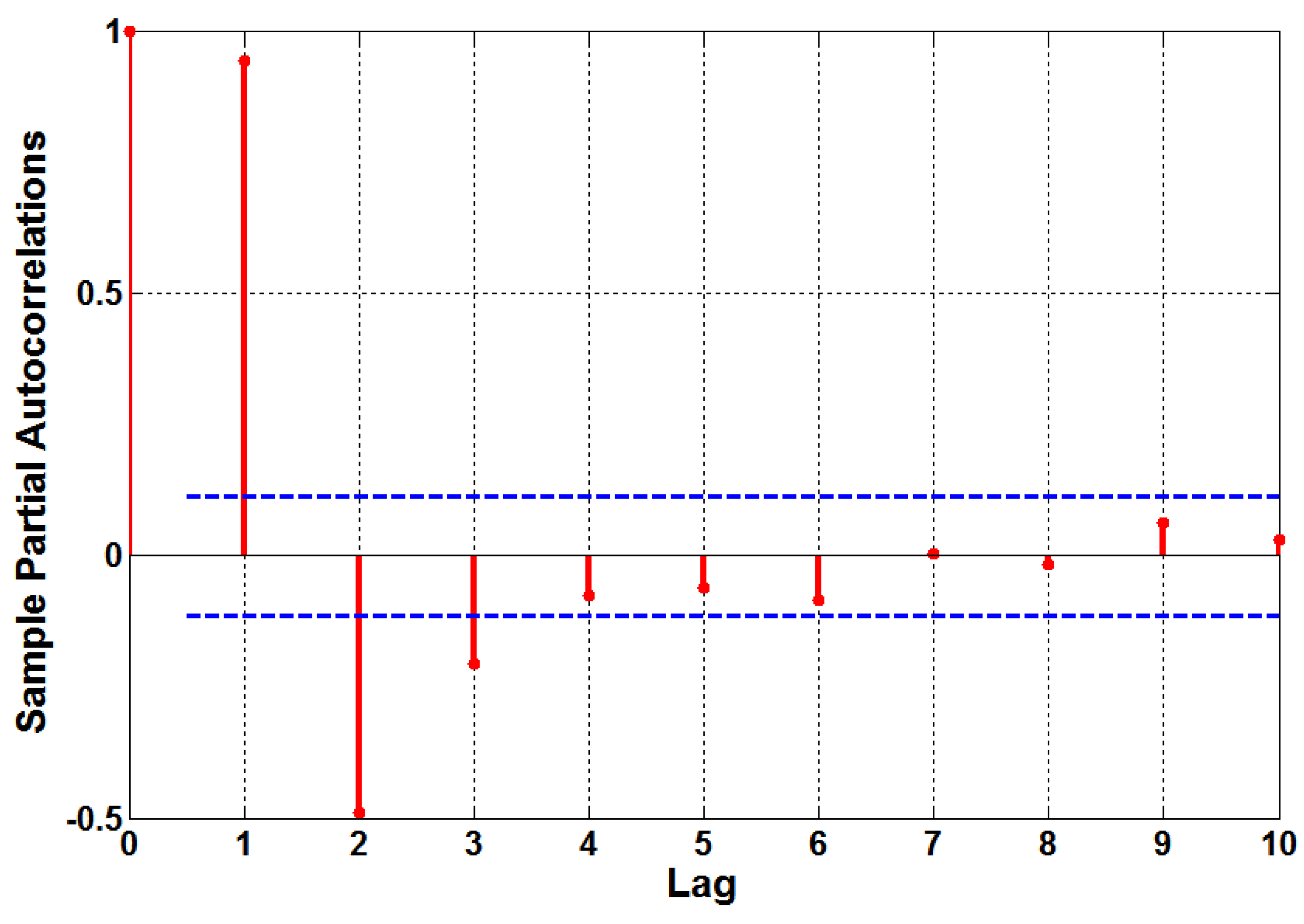
We decided the order of AR model as three, that is AR (3) model, after investigating the Pennsylvania-New Jersey-Maryland Interconnection (PJM) load data for the period from April to May 2013. We have confirmed that this model accurately reflects the load by analyzing the partial autocorrelation function. As shown in Figure 1, except for the first three points, the other points fall within the threshold limits (dashed line corresponding to 95% confidence) which tells us that the model represents the data very well. It can be interpreted that the output of AR (3) model will fall within the 95% confidence interval of the actual PJM data.

Figure 1. Partial autocorrelation function of load uncertainty.

Figure 1. Partial autocorrelation function of load uncertainty.

3. Unit Commitment Algorithms

3.1. Interruptible Load in Unit Commitment

In order to deal with the uncertainties in power system operation, such as load forecasting errors and equipment failure, power system operators must determine the commitment states of units to provide robustness and flexibility to the system. The most common method used by operators is to commit enough generators to provide a total capacity above the firm system demand and maintain a spinning reserve. In recent years, there have been a number of UC studies that have incorporated interruptible load into the spinning reserve [6]. The authors of these works include interruptible load in the objective function, and solve for the optimal amount of interruptible load. However, the computational time is increased by the additional variables to be optimized, and becomes especially burdensome when the procedure is applied to a complex power network.

In this paper, interruptible load is not considered in the objective function, nor do we allow it to directly affect the spinning reserve constraint. We propose a novel method for indirectly determining the required amount of interruptible load while achieving the desired level of reliability. The main idea of the method is illustrated in Figure 2. The bold line represents the expected load and the fine solid line indicates the possible increased load, which is the sum of the expected load and the spinning reserve. In a conventional UC method, enough generators should be turned on to exceed the expected load plus the spinning reserve. This is indicated by the dotted line in Figure 2; the dotted line is located above the fine line at all times. In the proposed method, represented by the dashed line, enough generators are committed to satisfy only the expected load level. If a lack of spinning reserve (LSR) occurs at some time (such as hour 10 to 11 and hour 20 to 21), the ISO can contract for an interruptible load whose volume is equal to the shaded section of the figure.

In what follows, we describe the formulation of the proposed method, as well as a detailed procedure an ISO can use to schedule generators efficiently and determine the optimal quantity of interruptible load.

Figure 2. Determination of interruptible load requirement.

Figure 2. Determination of interruptible load requirement.

3.2. Proposed Unit Commitment Formulation

Figure 3 shows a flow chart of the proposed UC considering interruptible load. The formulation consists of the following steps.

Figure 3. Flow chart of the proposed UC algorithm.

Figure 3. Flow chart of the proposed UC algorithm.

Step 1: Solve the following UC problem, determine the optimal commitment decision and dispatched volume of each unit, and then go to Step 2:

(5)

subject to:

(6)

(7)

(8)

Step 2: Calculate the lack of spinning reserve (LSR) for each hour using the following equation:

(9)

where:

(10)

If LSR_t is less than IL_max at all times, go to Step 3A; else define a set K, where each k_i ∈ K is an hour when LSR_ki is greater than IL_max, and go to Step 3B.

Step 3A: If LSR_t is greater than 0, allocate an interruptible load equal to the spinning reserve deficiency LSR_t, which is the value calculated in Step 2. Go to Step 4.

Step 3B: Assume that an interruptible load of IL_max is contracted at hour k, and solve the modified UC problem with constraint Equation (11) inserted. Go to Step 2.

Spinning reserve requirements:

(11)

where:

(12)

Step 4: The commitment states and power outputs of the generating units, as well as the amount of interruptible load to be contracted at every hour, are all determined.

In Step 1, the objective of Equation (5) is to minimize the total operating cost, consisting of the production cost plus startup cost. The constraints include the system power balance Equation (6) and the unit generation output limits Equation (7). In addition to the above constraints, each generating unit must be restricted by other constraints, such as unit status, ramp rate, network, and minimum up/down time constraints. Equation (8) implicitly covers all these constraints [15]. In this step, the decision variables are the commitment state and the power output of each generating unit. It should be noted that the quantity of interruptible load is not explicitly considered, and a spinning reserve constraint is not included in the above formulation.

After the commitment states and power outputs have been determined in Step 1, the lack of spinning reserve is calculated in Step 2, and the awarded volume of interruptible load is also obtained. In this step, the generator spinning reserve is restricted by the ramp rate limits. If it appears to be possible to contract for the calculated interruptible load, the ISO proceeds to obtain commitments for that volume. On the other hand, if the volume of interruptible load to be contracted exceeds IL_max, some generators must be turned on to provide spinning reserve. This is the procedure carried out in Step 3B. In this step, the newly inserted constraint changes the optimal UC results, and thus the output of each generator and interruptible load should be recalculated. This is why the return to Step 2 is necessary.

In the proposed approach, system operators can use interruptible load as an energy supply when there is insufficient spinning reserve from conventional generators. To put it another way, if the actual load demand is not much greater than the forecasted load, the system operator can respond to the increased demand with spinning reserve only, and the contracted interruptible loads remain a “reserve” in the literal sense of the word. Hence, system operators can reduce the probability of paying the high energy costs associated with interruptible loads, but still maintain the required level of spinning reserve by using a suitable amount of interruptible load.

4. Techniques for Solving the Proposed Unit Commitment Formulation

4.1. Lagrange Relaxation for Unit Commitment

We used the Lagrangian relaxation method in this paper since it offers numerous advantages over other techniques when applied to large power systems with many power sources. With the aid of this technique, we could decouple the problem into N subproblems, and solve the UC problem for each individual generator. A dual optimization procedure with Lagrange relaxation was used of the form:

(13)

where :

(14)

where:

(15)

It can be seen that the third term in Equation (14), which is related to the spinning reserve, is modified in contrast to the one found in the classic formulation. The Lagrangian relaxation method attacks the UC optimization problem in two steps. It first maximizes q(λ_t,μ_t) with respect to the Lagrange multipliers. The Lagrangian function L(U,P,λ,μ) is then minimized with respect to the variables U and P for fixed values of the Lagrange multipliers. We can rewrite the Lagrangian function as:

(16)

The last two terms in Equation (16) are constant with respect to U and P, and thus they can be dropped when solving the minimization problem. Finally, we can express the Lagrangian function as:

(17)

The most important aspect of Equation (17) is that the generating unit functions are separated from each other, as in the conventional approach. Consequently, we can solve the optimization problem by separately minimizing each individual generator unit, as we expected. In what follows, we give a brief description of the dynamic programming method used to solve each of the single-generator subproblems.

4.2. Dynamic Programming for Single-Unit Optimization

We solved the single-generator optimization problem by utilizing dynamic programming, which is based on the principle of optimality. The optimal UC decision made in the last period of the problem was taken to be optimum for the entire problem [16]. Thus, we determined the optimal policy for the last period, and proceeded backward in time to find the optimal status of the unit in each of the previous periods.

In this study, it was assumed that a generator had been on/off longer than the minimum on/off time requirement at the starting point of the problem. Hence, it could be turned off/on immediately after one time period. However, note that if a generator has been on/off for less than the minimum time requirement, its state should be maintained in order to satisfy the minimum on/off time constraint.

In the following section, we present numerical results for three scenarios. In the first scenario, it is assumed that the load is perfectly forecasted, which means that uncertainty is ignored. The second scenario demonstrates the effect of load uncertainty. In the last scenario, we simulate a case where wind turbines are interconnected with the grid. How wind speed uncertainties affect the optimal spinning reserve is analyzed, and the effects of different levels of wind penetration are also examined.

5. Numerical Results

We assessed two different UC policies: a conventional UC policy that does not consider interruptible load and the proposed UC policy that uses interruptible load. In order to analyze these policies, we calculated the expected total operating cost and the expected energy not supplied by applying a Monte Carlo simulation approach, where the number of samples was 1000 [15]. Although the Monte Carlo approach imposes a computational burden, it can readily accommodate a wide range of probability distributions [17].

As described in Section 2, it was assumed that the wind speed followed an ARMA (p,q) model, where p = 3 and q = 2. The autoregressive order p was set to 1.7901, 0.9087, 0.0948, and the moving average term q was 1.0929, 0.2892. These parameters were obtained from [13]. The AR (3) model represented the load uncertainty; the values of used in the model were 0.9427, 0.4896, 0.2060. We added this uncertainty term to the expected load to calculate the actual load.

Taking wind power and load into account, the IEEE 118-bus test system was used to assess the proposed UC [18]. This system consists of 54 generators and 24 hourly loads are specified, with a peak load of 6000 MW occurring at hour 21. The specifications of the wind turbines considered in this paper are the following: rated power of 5 MW, cut-in speed of 3 m/s, rated speed of 11.4 m/s, cut-out speed of 25 m/s, rotor diameter of 112 m and hub height of 90 m. The other details can be found in [14]. When we solve a UC problem, the ramp rate and minimum on/off time are dependent on the test system. Here, all units were assumed to be free from must-run or must-not-run statuses at all times. The energy cost of the interruptible load was assumed to be $60/MWh, and the contract cost was set to $4/MWh. The detailed generator costs are given in [18].

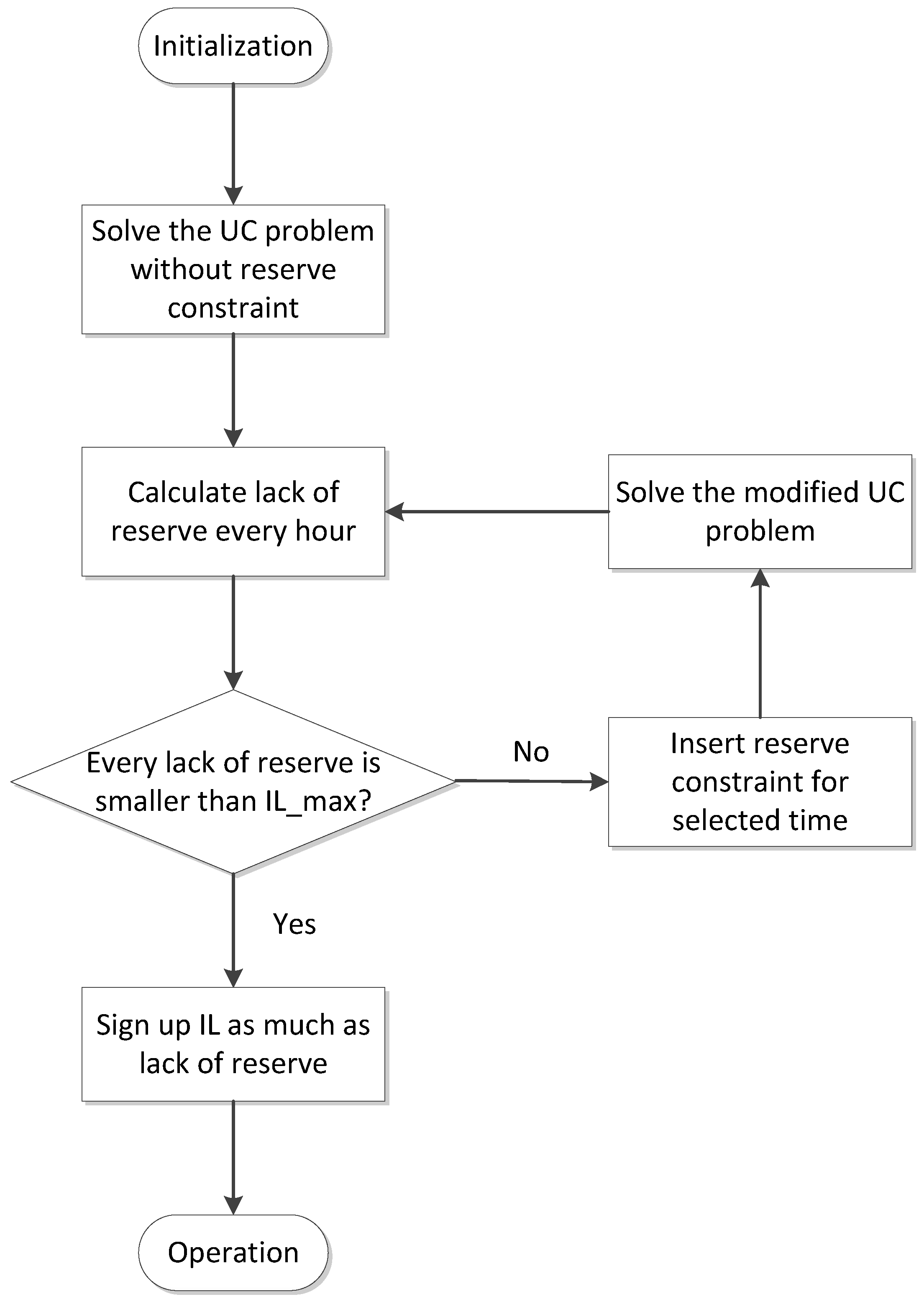
We analyzed several cases using both the conventional and proposed approaches. Before comparing the two techniques, we discuss an intermediate result of using our method. As described above, in our method, the UC problem is first solved without spinning reserve constraints, and the required interruptible load contracts are then computed. Table 1 shows the resulting unintentionally acquired spinning reserves and the corresponding deficits in the reserve requirement when it was set to 5% of the peak load. In this case, each LSR_t was within the upper limit of IL_max, and thus the ISO could contract any amount of interruptible load up to LSR_t. Using these contracts, the ISO was able to cope with the variability in system operation, and reserve shortage situations were not likely to happen, even if the spinning reserve was given no consideration in the UC problem. The expected energy not supplied (EENS) was used as a reliability criterion expressed in terms of UC discrete and continuous variables, based on the LR-DP method.

Table 1. Acquired spinning reserve and resultant deficits in reserve requirement.

Time (h)	Acquired Spinning Reserve (MW)	Lack of Spinning Reserve (MW)	IL Contract Volume (MW)
1	600	0	0
2	663.12	0	0
3	788.03	0	0
4	1085	0	0
5	1349.8	0	0
6	1214	0	0
7	1067.1	0	0
8	975	0	0
9	801.83	0	0
10	622.81	0	0
11	596.89	0	0
12	713.63	0	0
13	910	0	0
14	975	0	0
15	622.6	0	0
16	576.38	0	0
17	692.1	0	0
18	599.52	0	0
19	460.12	0	0
20	248.16	51.84	51.84
21	195	105	105
22	610.77	0	0
23	679.29	0	0
24	152.5	147.5	147.5

Table 1. Acquired spinning reserve and resultant deficits in reserve requirement.

Time (h)	Acquired Spinning Reserve (MW)	Lack of Spinning Reserve (MW)	IL Contract Volume (MW)
1	600	0	0
2	663.12	0	0
3	788.03	0	0
4	1085	0	0
5	1349.8	0	0
6	1214	0	0
7	1067.1	0	0
8	975	0	0
9	801.83	0	0
10	622.81	0	0
11	596.89	0	0
12	713.63	0	0
13	910	0	0
14	975	0	0
15	622.6	0	0
16	576.38	0	0
17	692.1	0	0
18	599.52	0	0
19	460.12	0	0
20	248.16	51.84	51.84
21	195	105	105
22	610.77	0	0
23	679.29	0	0
24	152.5	147.5	147.5

However, if the ISO decided to procure a spinning reserve that amounted to 7% of the peak load, the required volume of interruptible load exceded IL_max, and more committed generators were needed to satisfy the reserve prerequisite. Table 2 shows the resulting reserve deficits; the spinning reserve could not be fully covered by the interruptible load at hours 20, 21, and 24. Accordingly, the UC problem must be solved again, taking spinning reserve constraints into account at these hours; the results are listed in the third column of Table 2. It can be seen that each LSR_t value was less than IL_max. Even if it was assumed that IL_max was used as the level of spinning reserve in the UC problem, the interruptible load ultimately awarded was completely different from IL_max. The reason for this was that the dispatched volume of each generator was changed significantly by the newly inserted constraint, and the resultant lack of reserve was also modified.

Table 2. Results of spinning reserve with and without consideration of reserve requirement.

Time (h)	Lack of Spinning Reserve (MW)		IL Contract Volume (MW)
	without Reserve Constraint	with Reserve Constraint
20	171.84	0	0
21	225	81.22	81.22
24	267.5	122.5	122.5

Table 2. Results of spinning reserve with and without consideration of reserve requirement.

Time (h)	Lack of Spinning Reserve (MW)		IL Contract Volume (MW)
	without Reserve Constraint	with Reserve Constraint
20	171.84	0	0
21	225	81.22	81.22
24	267.5	122.5	122.5

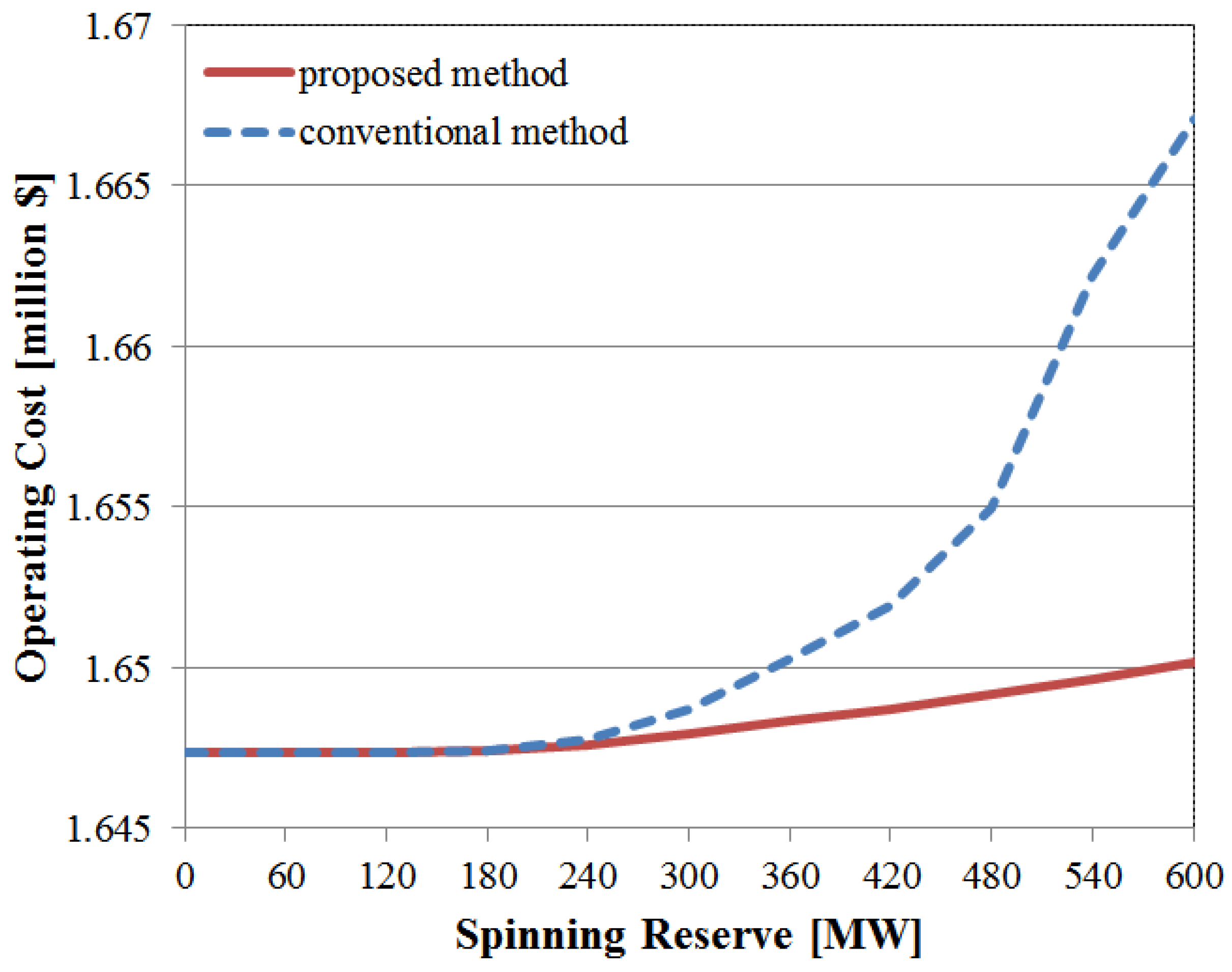
We calculated the expected operating costs using the above procedure, and compared the results with those obtained via the conventional UC approach. First, to isolate the effect of securing reserve on the cost, load uncertainty was not considered. In other words, it was assumed that the load was forecasted perfectly. In the conventional method, the operating cost is based solely on the generation cost, whereas in the proposed method, the operating cost comprises the generation cost and the interruptible load contract cost. The operating cost for each UC method is shown in Figure 4. In both methods, the operating cost escalated as the spinning reserve increased. However, the cost increased more drastically when the conventional method was applied to the UC problem. The main reason for this was that more units were dispatched for the purpose of securing reserve. The startup costs of these newly introduced units were added directly to the operating cost, and the altered arrangement of committed generators also indirectly boosted the cost. When the problem was solved using tailored interruptible load contracts, the cost increased smoothly. This was due to the fact that production and startup costs rarely change with respect to the requirement level, and thus the operating cost was mainly affected by the awarded amount of interruptible load.

Figure 4. Operating cost comparison with the conventional method.

Figure 4. Operating cost comparison with the conventional method.

The total number of generators committed to supply the load and the dispatched output are given in Table 3 for the case when the spinning reserve requirement was set to 7% of the peak load. When the proposed method was used, few units were turned off, especially at peak load time. As described above, the dispatched output of each generator was also changed to minimize the operating costs. The third column on the right of Table 3 lists the dispatched outputs of units 10 and 30. It can be seen that the proposed method made greater use of the cost-effective unit 10, while the outputs of the more expensive units, such as unit 30, were reduced.

Table 3. Results of unit commitment in conventional method and proposed method.

Time (h)	Total Number of Committed Generators		Dispatched Volume of Unit 10 (MW)		Dispatched Volume of Unit 30 (MW)
	Proposed Method	Conventional Method	Proposed Method	Conventional Method	Proposed Method	Conventional Method
1	17	17	201.34	201.39	0	0
2	17	17	179.24	179.24	0	0
3	17	17	132.67	132.67	0	0
4	17	17	100	100	0	0
5	32	32	100	100	0	0
6	32	32	107.82	107.82	0	0
7	32	32	169.75	169.75	0	0
8	32	32	218.21	218.25	0	0
9	32	32	246.53	246.52	0	0
10	32	32	269.02	269.02	0	0
11	32	32	271.9	271.9	0	0
12	32	32	257.47	257.47	0	0
13	32	32	233.23	233.24	0	0
14	32	32	203.24	203.28	0	0
15	32	32	269.01	269.01	0	0
16	33	32	273.06	274.83	35.745	0
17	33	32	258.74	260.36	32.847	0
18	33	32	270.18	271.94	35.58	0
19	42	33	279.74	291.79	37.27	30
20	47	33	289.24	296.07	40.202	38.327
21	51	44	293.3	300	40.956	30
22	33	33	273.03	273.03	36.384	36.384
23	33	33	264.46	264.46	34.052	34.052
24	39	35	269.26	300	30	30

Table 3. Results of unit commitment in conventional method and proposed method.

Time (h)	Total Number of Committed Generators		Dispatched Volume of Unit 10 (MW)		Dispatched Volume of Unit 30 (MW)
	Proposed Method	Conventional Method	Proposed Method	Conventional Method	Proposed Method	Conventional Method
1	17	17	201.34	201.39	0	0
2	17	17	179.24	179.24	0	0
3	17	17	132.67	132.67	0	0
4	17	17	100	100	0	0
5	32	32	100	100	0	0
6	32	32	107.82	107.82	0	0
7	32	32	169.75	169.75	0	0
8	32	32	218.21	218.25	0	0
9	32	32	246.53	246.52	0	0
10	32	32	269.02	269.02	0	0
11	32	32	271.9	271.9	0	0
12	32	32	257.47	257.47	0	0
13	32	32	233.23	233.24	0	0
14	32	32	203.24	203.28	0	0
15	32	32	269.01	269.01	0	0
16	33	32	273.06	274.83	35.745	0
17	33	32	258.74	260.36	32.847	0
18	33	32	270.18	271.94	35.58	0
19	42	33	279.74	291.79	37.27	30
20	47	33	289.24	296.07	40.202	38.327
21	51	44	293.3	300	40.956	30
22	33	33	273.03	273.03	36.384	36.384
23	33	33	264.46	264.46	34.052	34.052
24	39	35	269.26	300	30	30

Next, we examined the two UC approaches in an uncertain environment. When load and wind uncertainties are considered, cases arise in which the spinning reserve is used for energy production. If this reserve is inadequate to cover a sudden demand increase, the ISO must specify an amount of load shedding, which was set to $1000/MWh in this paper. In order to find the optimal reserve rate, we employed a Monte Carlo simulation, in which the rate of the reserve was adjusted in steps of 0.01% of the peak load.

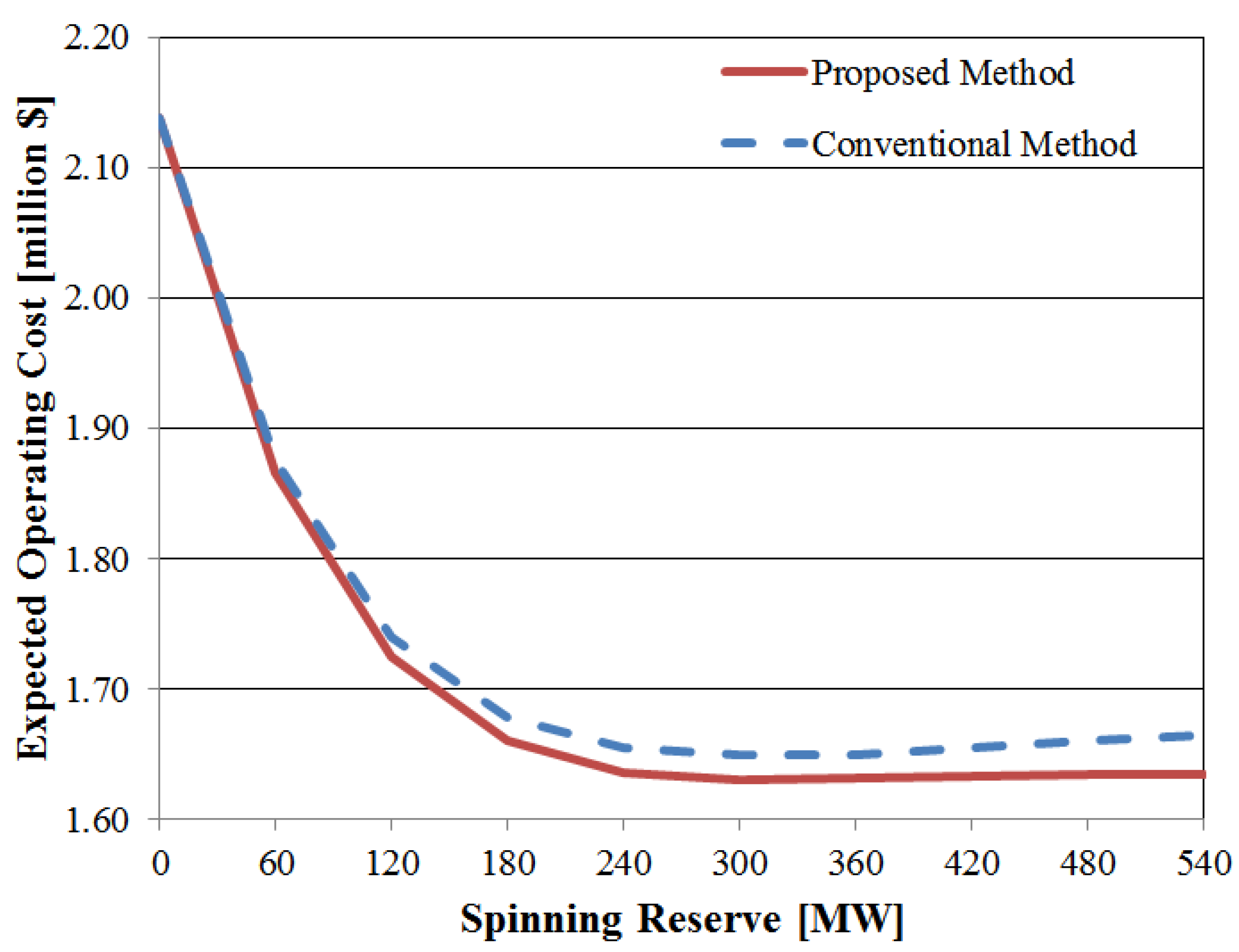
Figure 5 shows the expected total cost when load uncertainty is considered. In the conventional technique, the expected total cost comprises the generation and load-shedding costs. If interruptible load is also considered in the problem, its cost is added to the total cost. As the load-shedding costs dramatically decreased, the total cost also declined to a certain point, since much more spinning reserve was provided. Beyond the optimal point, the cost increased slightly because the benefits obtained from decreasing load-shedding costs could not offset the incremented reserve costs the ISO must pay. By using a new method to procure the reserve at a comparatively lower cost, the ISO could reduce the operating cost with a greater reserve rate. This also could be interpreted as ISO mitigation of the load-shedding risk without changing the cost. 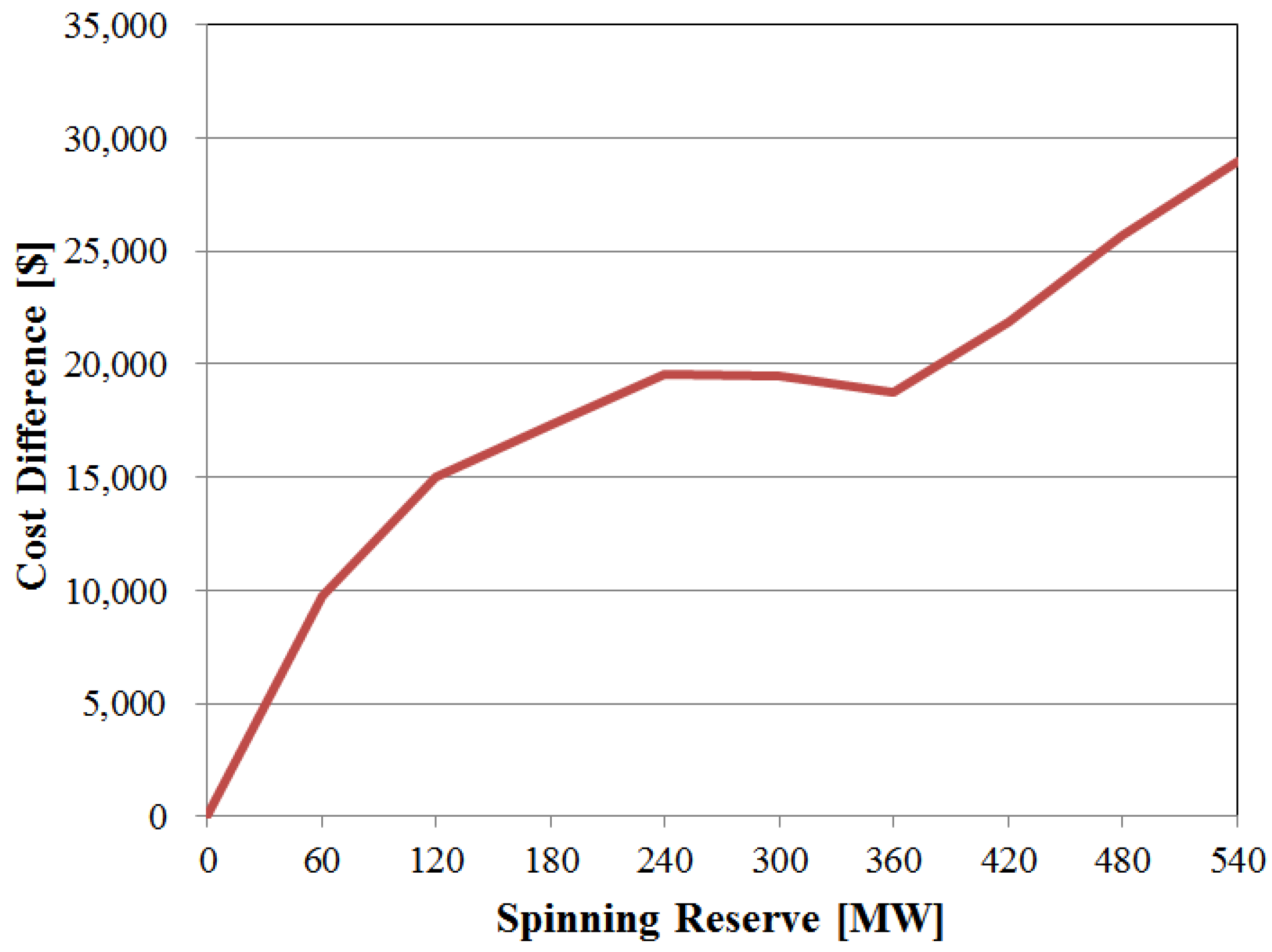Figure 6 highlights the gap between the total costs obtained from the two UC approaches, and verifies that consideration of the interruptible load in a UC problem is especially beneficial when a higher reserve is needed.

Figure 5. Expected operating cost according to spinning reserve.

Figure 5. Expected operating cost according to spinning reserve.

Figure 6. Cost difference in the conventional method and proposed method.

Figure 6. Cost difference in the conventional method and proposed method.

Table 4 summarizes the optimal reserve rates and corresponding expected costs for each method. As the table indicates, the actual usage costs of the contracted interruptible loads were modest compared to their capacity costs. The usage costs of these interruptible loads hardly affected the total operating cost because the spinning reserve from online generators was exhausted before interruptible load was utilized.

Table 4. Optimal reserve and cost in conventional method and proposed method.

Method	Proposed Method	Conventional Method
Optimal reserve requirement (MW)	300	300
Generation costs ($)	1,626,261	1,647,476
Load shedding costs ($)	2301	2301
IL capacity costs ($)	1346	-
IL usage costs ($)	389	-
Expected total costs ($)	1,630,298	1,649,778
Cost savings compared to conventional method ($)	19,480 (1.19%)	-

Table 4. Optimal reserve and cost in conventional method and proposed method.

Method	Proposed Method	Conventional Method
Optimal reserve requirement (MW)	300	300
Generation costs ($)	1,626,261	1,647,476
Load shedding costs ($)	2301	2301
IL capacity costs ($)	1346	-
IL usage costs ($)	389	-
Expected total costs ($)	1,630,298	1,649,778
Cost savings compared to conventional method ($)	19,480 (1.19%)	-

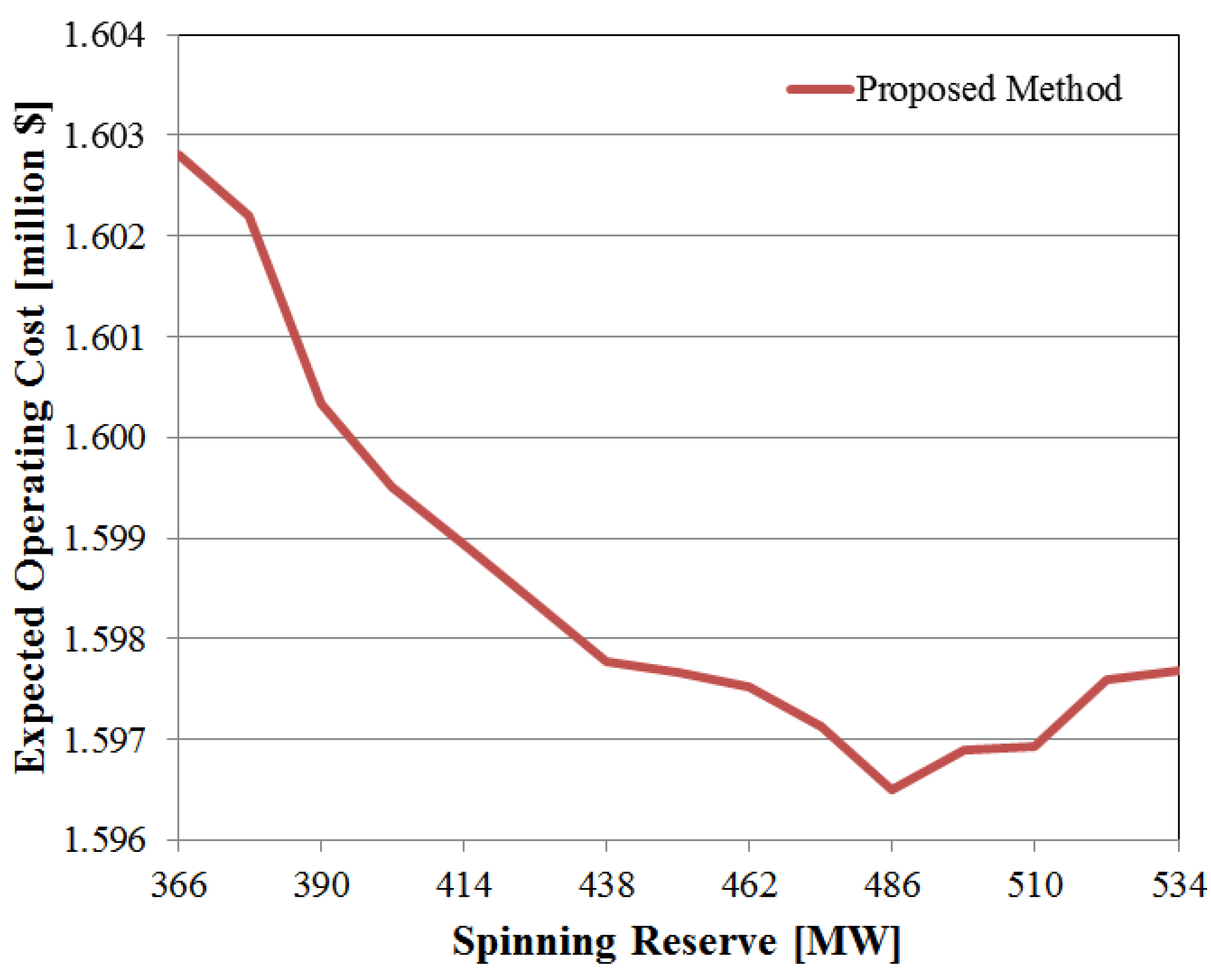
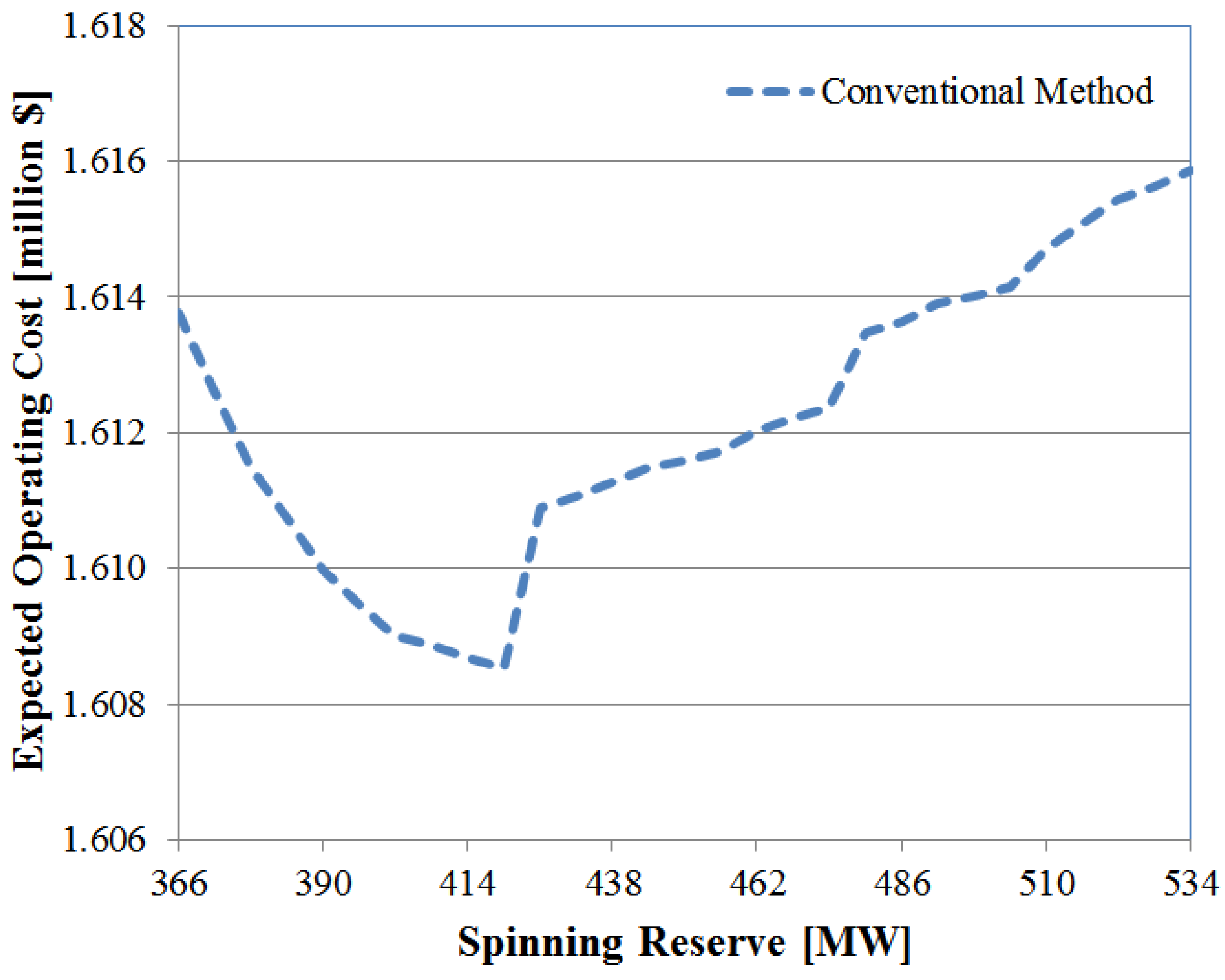
As described in the introduction, more emphasis needs to be placed on reserve costs when a wind farm is integrated into a power system. Figure 7 and Figure 8 show the expected total cost when wind power is implemented. It was assumed that the total wind power capacity was 15% of the peak load. In order to reveal the detailed shape of the cost function, we enlarged the graphs in the region near the optimal point. The optimal points of both graphs were slightly shifted to the right in comparison with the optimal points of Table 4, which means that the ISO required a larger spinning reserve to deal with uncertainties in both the loads and the wind power output. Since the generation costs associated with wind generation were ignored, the expected total cost was lower than the cost accrued without wind power, in spite of the greatly increased load-shedding costs.

Figure 7. Expected operating cost and optimal spinning reserve in the proposed method.

Figure 7. Expected operating cost and optimal spinning reserve in the proposed method.

Figure 8. Expected operating cost and optimal spinning reserve in the conventional method.

Figure 8. Expected operating cost and optimal spinning reserve in the conventional method.

Figure 9 and Table 5 show the optimal reserve rates and minimum expected costs at different wind penetration levels. The cost effectiveness of the proposed method was evident in all cases, but the cost reduction benefits were less likely to occur when the wind penetration was high. This was due to the difference in the reserve rates of the two methods and underestimation of the load-shedding costs. When a limitation on the expected energy not supplied (EENS) was imposed on the UC problem, the proposed method was highly beneficial. This is verified in Table 5, which lists the minimum expected costs when the EENS was held below 1 MWh. In this case, the ISO could reduce the total cost to $18,871 by properly utilizing interruptible load when the wind penetration level was 20%.

Figure 9. Expected operating cost and optimal reserve with various wind penetration level.

Figure 9. Expected operating cost and optimal reserve with various wind penetration level.

Table 5. Expected operating costs and cost savings when expected energy not supplied (EENS) is limited within 1 MWh.

Wind power Penetration Level (%)	Expected Operating Costs ($)		Cost Savings ($)
	Proposed Method	Conventional Method
5	1,619,278	1,635,997	16,718 (1.03%)
10	1,608,451	1,624,569	16,118 (1.00%)
15	1,595,148	1,612,700	17,551 (1.10%)
20	1,581,727	1,600,598	18,871 (1.19%)

Table 5. Expected operating costs and cost savings when expected energy not supplied (EENS) is limited within 1 MWh.

Wind power Penetration Level (%)	Expected Operating Costs ($)		Cost Savings ($)
	Proposed Method	Conventional Method
5	1,619,278	1,635,997	16,718 (1.03%)
10	1,608,451	1,624,569	16,118 (1.00%)
15	1,595,148	1,612,700	17,551 (1.10%)
20	1,581,727	1,600,598	18,871 (1.19%)

Lastly, the computational time required to solve the UC problem via each of the two approaches was evaluated. The computational time was measured on a core 2 Duo E7200, 2.53 GHz, with 2.00 GB of random access memory (RAM). In the conventional method, there are two Lagrangian multipliers, corresponding to the reserve constraint and balance-of-supply-and-demand constraint. Both multipliers must be updated iteratively until the costs are fully minimized while satisfying the reserve constraint. On the other hand, in the proposed method, only one multiplier is considered in the UC, and the reserve constraint is ignored in the main problem. This can reduce the computational time sufficiently to offset the additional runtime required to calculate the contracted volume of interruptible load. Table 6 lists the average computational times for the different methods with a sample size of 100. It is not accidental that the computational time advantage was more noticeable when the reserve rate was high since more iterations were needed to satisfy a high reserve requirement in the conventional method.

Table 6. Computational time with respect to spinning reserve level.

Spinning Reserve (%)	Computational Time (s)
	Conventional Method	Proposed Method
5	35.20	27.26
10	100.34	54.91

Table 6. Computational time with respect to spinning reserve level.

Spinning Reserve (%)	Computational Time (s)
	Conventional Method	Proposed Method
5	35.20	27.26
10	100.34	54.91

6. Conclusions

The probabilistic nature of renewable energy, especially wind energy, increases the need for new kinds of operational schemes for power systems. In particular, operating reserve requirements must be revised in order to maintain a desired system reliability level in an uncertain operating environment. This paper proposes a daily UC that utilizes interruptible load to deal with the increased uncertainty due to wind power. Load and wind generation are treated as uncertainty sources, and are assumed to follow a normal distribution. The expected energy not supplied (EENS) is regarded as a reliability criterion. LR-DP was adopted to solve the proposed UC problem efficiently. The performance of the proposed UC was verified using an IEEE 118-bus system with wind farms. The simulation results clearly demonstrated that with demand-side participation, a system operator could reduce the operating cost significantly when handling the increased uncertainty due to wind power integration within desired reliability criteria. The cost saving effect for stable system operation became remarkable, especially at higher wind power penetration levels. Moreover, the computational time, which is a crucial factor for short-term generation-scheduling tools, could be shortened by using the proposed approach.