
Stability Analysis of Methane Hydrate-Bearing Soils Considering Dissociation

Abstract
:1. Introduction


2. One-Dimensional Instability Analysis of Methane Hydrate Bearing Viscoplastic Material
2.1. Governing Equations
2.1.1. General Settings
2.1.2. Stress Variables
2.1.3. Conservation of Mass
2.1.4. Balance of Momentum
2.1.5. Darcy Type of Law
2.1.6. Conservation of Energy
2.1.7. Dissociation Rate of Methane Hydrates
2.1.8. Simplified Viscoplastic Constitutive Model
2.2. Perturbed Governing Equations
2.3. Conditions of Onset of Material Instability
2.3.1. Sign for the Coefficients and
- (A)
- : compressive strain
- (1)
- When parameter is positive, that is, the viscoplastic hardening, the term in is always positive. The sign for always becomes positive:
- (2)
- When the parameter is negative, that is, the viscoplastic softening, becomes negative, if it satisfies the following inequality:The material instability might occur even if it is viscoplastic hardening material.
- (B)
- : expansive strain
- (3)
- When parameter is positive, that is, the viscoplastic hardening, the term in becomes negative, if it satisfies the following inequality:
- (4)
- When parameter is negative, that is, viscoplastic softening, the term is always negative. Thus, the sign for is always negative. This may lead to the material instability, because it does not satisfy the first condition of the Routh-Hurwitz criteria:
2.3.2. Sign for the Coefficients and
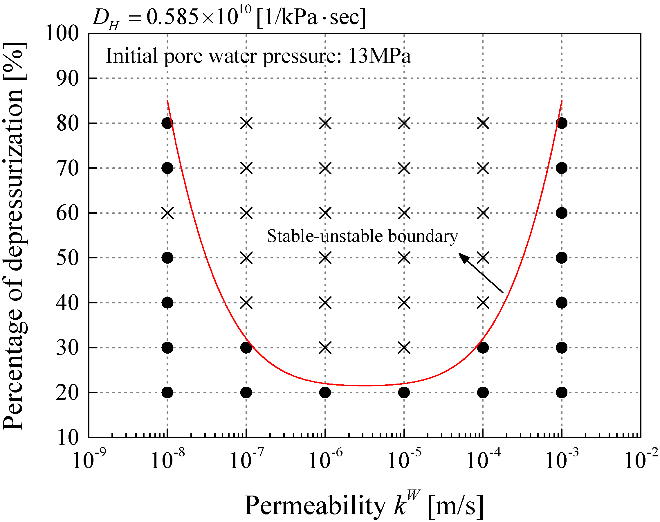
- In the case of large values for , , and , can become positive more easily. In contrast, low permeabilities for water and gas make the material system unstable.
3. Numerical Simulation of Instability Analysis by an Elasto-Viscoplastic Model Considering Methane Hydrate Dissociation
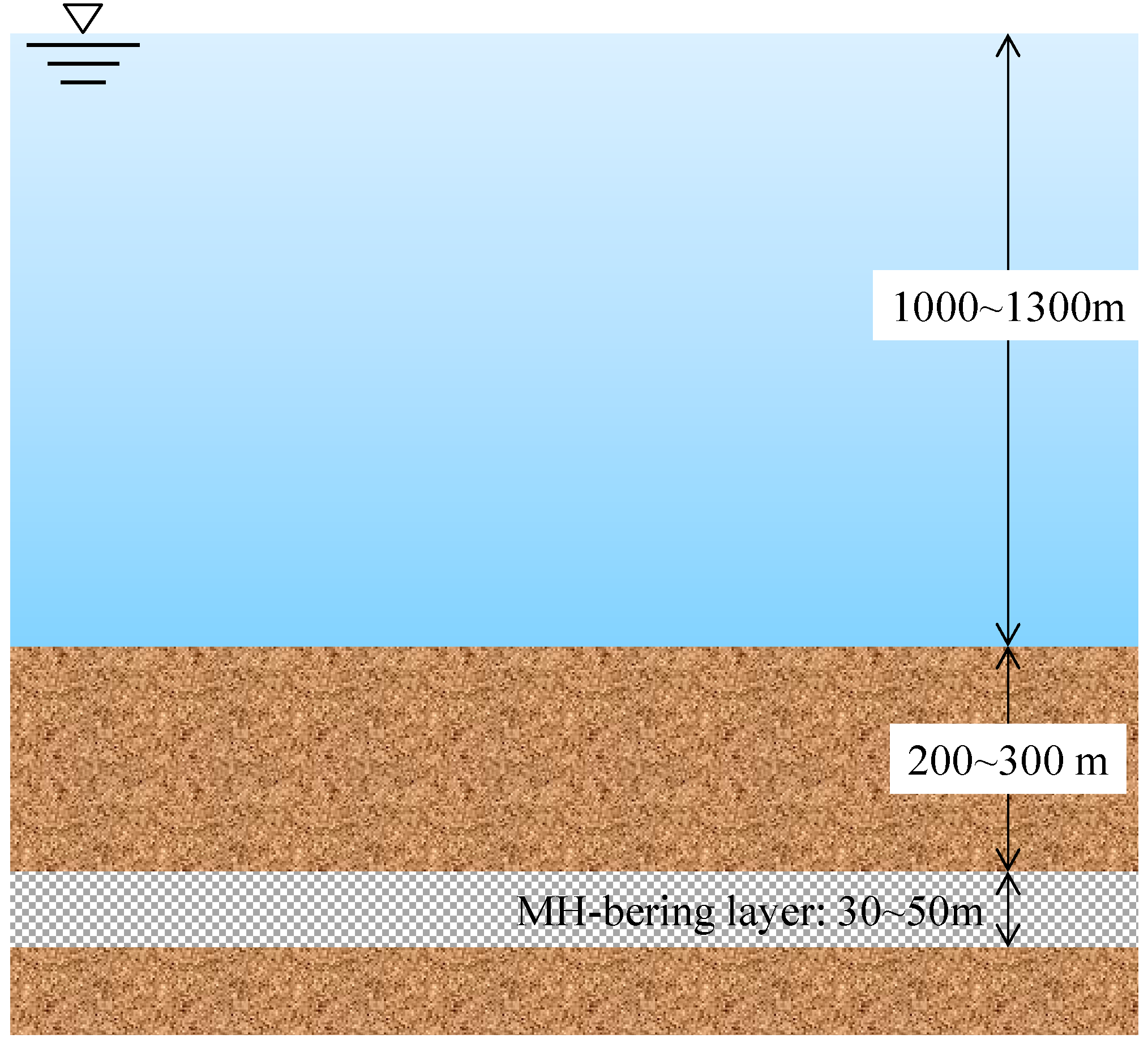
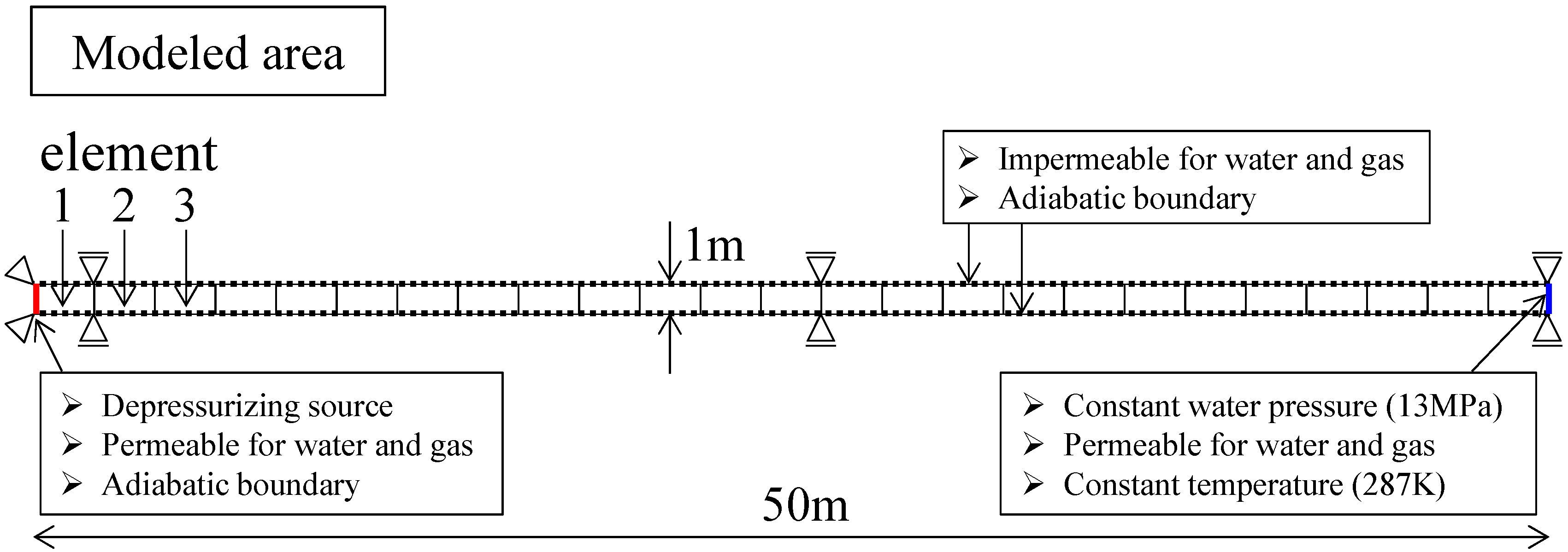
3.1. One-Dimensional Finite Element Mesh and Boundary Conditions


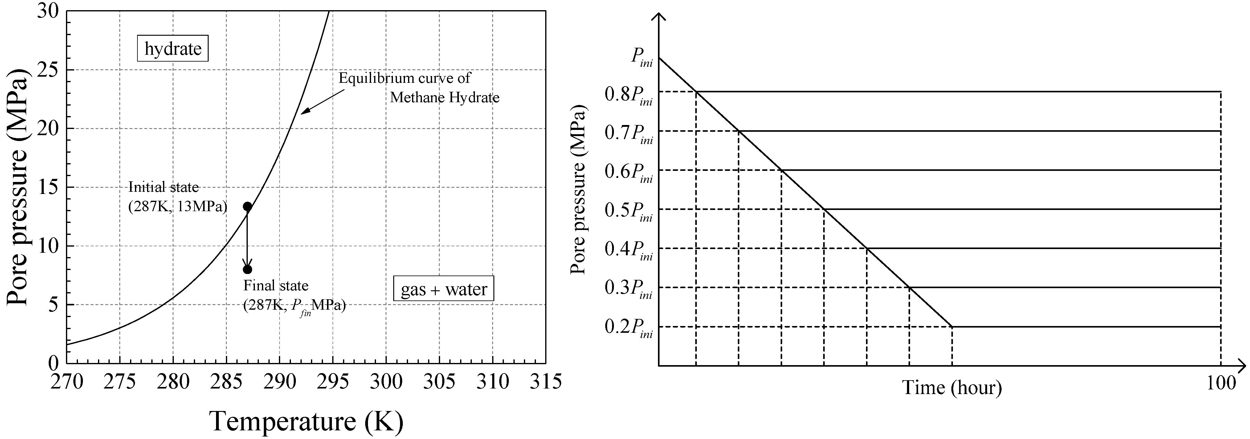
3.2. Initial and Simulation Conditions

| Name | Paremeter | Value |
|---|---|---|
| Initial Void Ratio | 1.00 | |
| Initial water saturation | 1.0 | |
| Initial hydrate saturation | 0.51 |
| Name | Parameter | Value |
|---|---|---|
| Compression Index | 0.185 | |
| Swelling index | 0.012 | |
| Initial shear elastic modulus (kPa) | 53,800 | |
| Viscoplastic parameter (1/s) | 1.0 × 10⁻¹⁰ | |
| Viscoplastic parameter | 23.0 | |
| Stress ratio at critical state | 1.09 | |
| Compression yield stress (kPa) | 1882 | |
| Degradation parameter | 1.0 | |
| Degradation parameter | 0.0 | |
| Parameter for suction effect (kPa) | 100 | |
| Parameter for suction effect | 0.2 | |
| Parameter for suction effect | 0.25 | |
| Parameter for hydrate effect | 0.51 | |
| Parameter for hydrate effect | 0.6 | |
| Parameter for hydrate effect | 0.75 | |
| Thermo-viscoplastic parameter | 0.15 | |
| Permeability coefficient for water (m/s) | variable | |
| Permeability coefficient for gas (m/s) | ||
| Permeability reduction parameter | 7 |

| Name | Values | Permeability (m/s) | |||||
|---|---|---|---|---|---|---|---|
| 1.0 × 10⁻³ | 1.0 × 10⁻⁴ | 1.0 × 10⁻⁵ | 1.0 × 10⁻⁶ | 1.0 × 10⁻⁷ | 1.0 × 10⁻⁸ | ||
| Degree of depressurization | 20% | Case-3-20 | Case-4-20 | Case-5-20 | Case-6-20 | Case-7-20 | Case-8-20 |
| 30% | Case-3-30 | Case-4-30 | Case-5-30 | Case-6-30 | Case-7-30 | Case-8-30 | |
| 40% | Case-3-40 | Case-4-40 | Case-5-40 | Case-6-40 | Case-7-40 | Case-8-40 | |
| 50% | Case-3-50 | Case-4-50 | Case-5-50 | Case-6-50 | Case-7-50 | Case-8-50 | |
| 60% | Case-3-60 | Case-4-60 | Case-5-60 | Case-6-60 | Case-7-60 | Case-8-60 | |
| 70% | Case-3-70 | Case-4-70 | Case-5-70 | Case-6-70 | Case-7-70 | Case-8-70 | |
| 80% | Case-3-80 | Case-4-80 | Case-5-80 | Case-6-80 | Case-7-80 | Case-8-80 | |
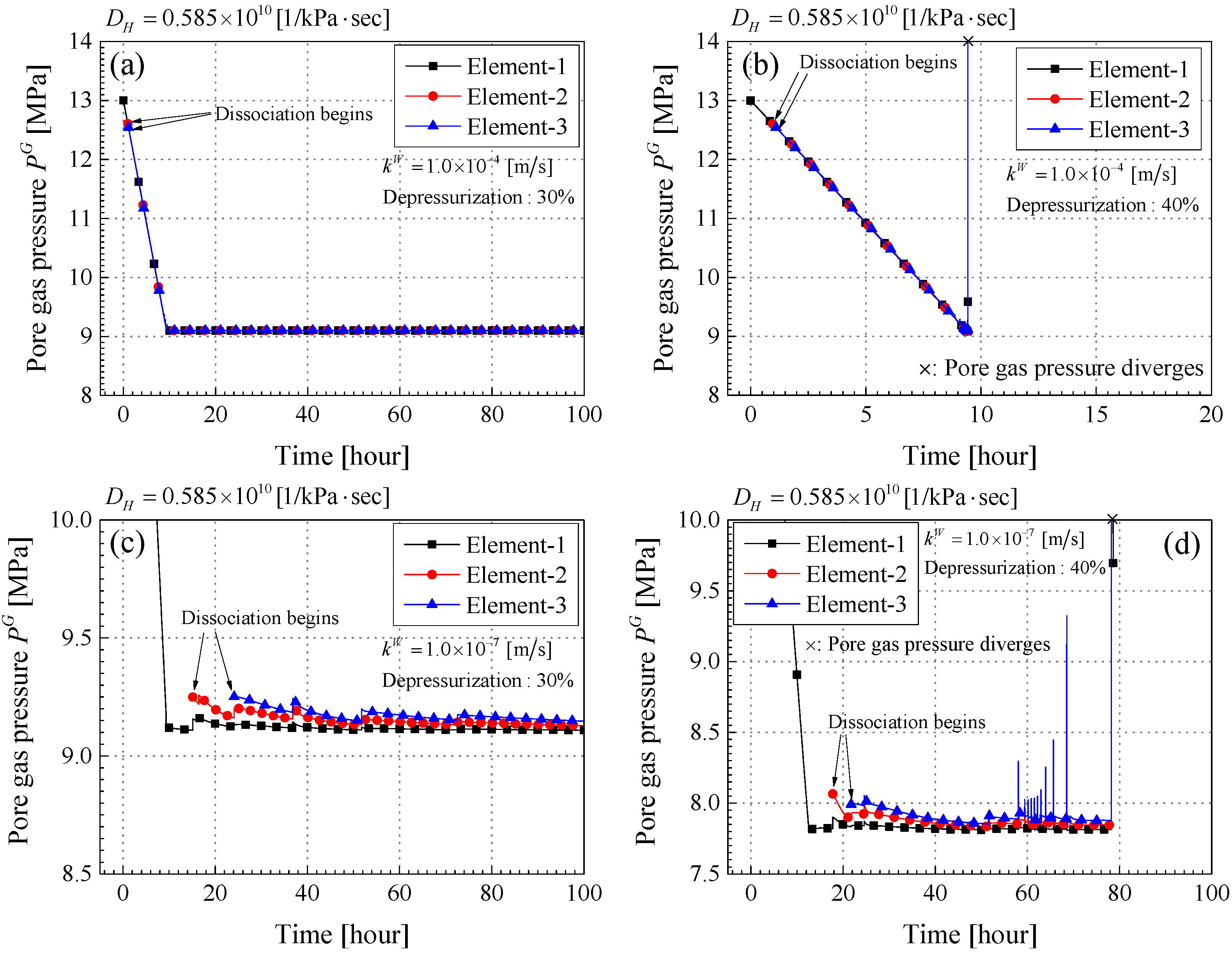
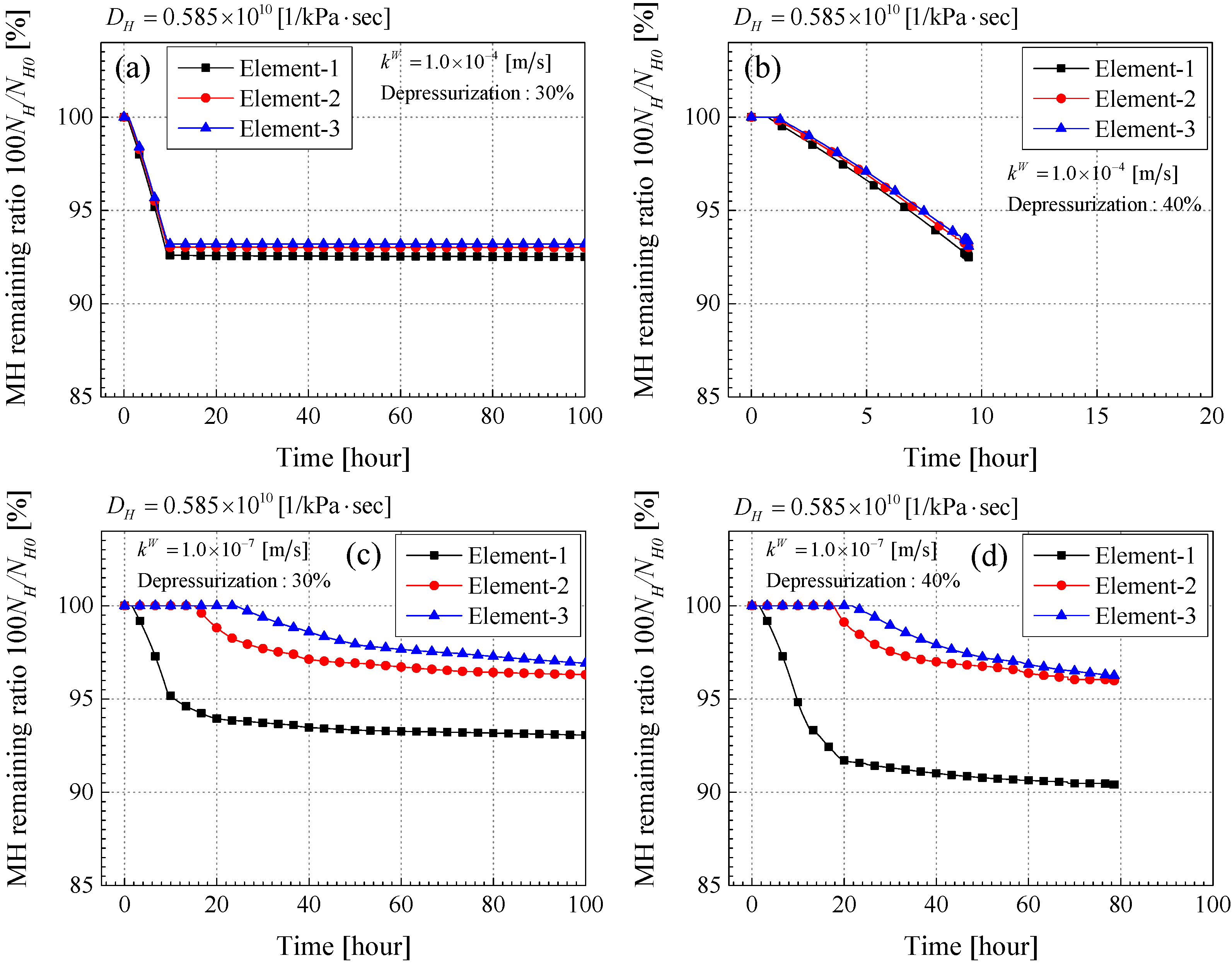
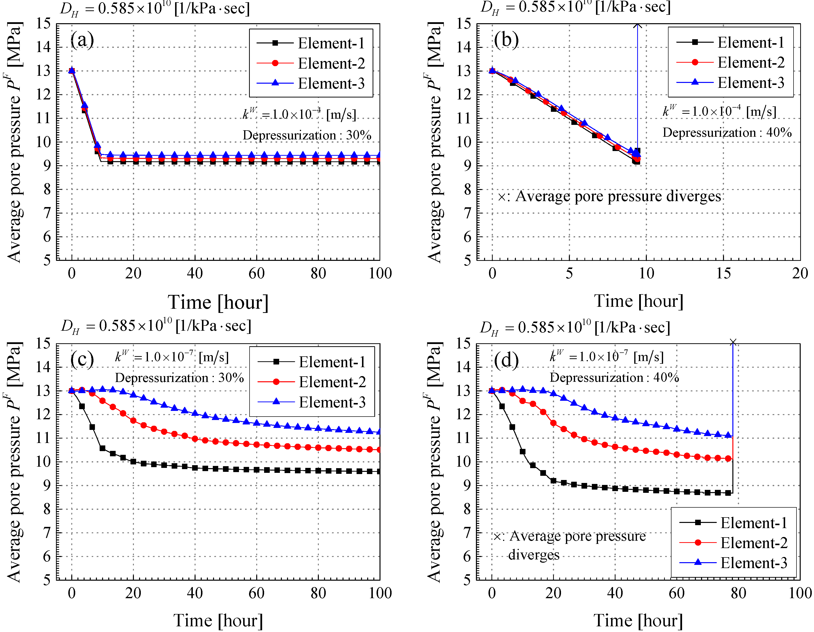
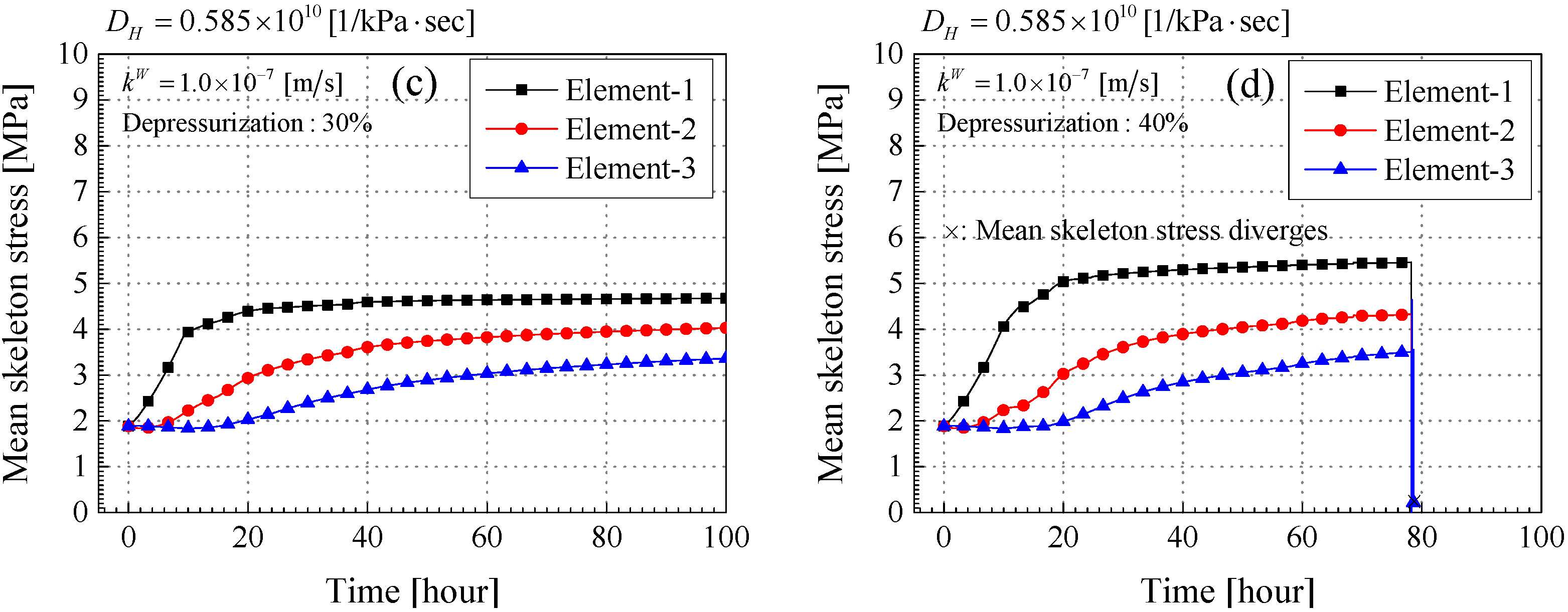
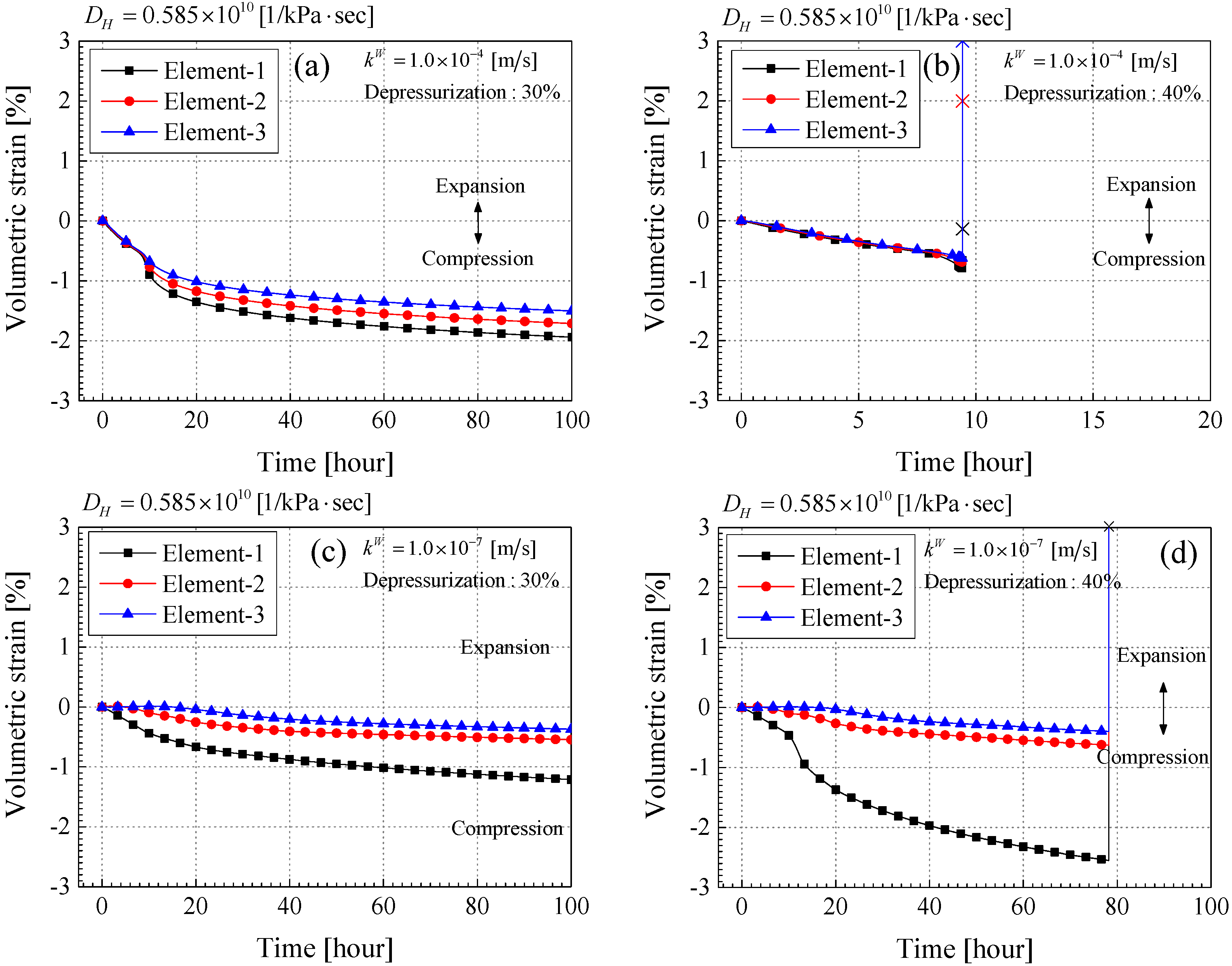
3.3. Simulation Results
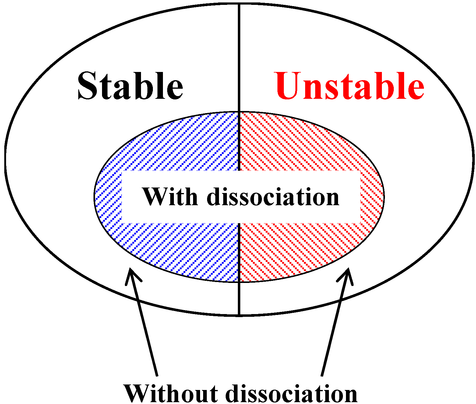
Results of the Stable-Unstable Behavior during MH Dissociation


| Variable | Value |
|---|---|
| vW | 8.4 × 10⁻⁶ m/s |
| D50 | 0.15 mm |
| vW (5 °C, 10 MPa) | 1.52 × 10⁻⁶ m2/s |
| Variable | Value |
|---|---|
| vG | 8.4 × 10⁻⁵ m/s |
| 0.15 mm | |
| vG (5 °C, 10 MPa) | 1.72 × 10⁻⁷ m2/s |


4. Conclusions
- The parameters which have a significant influence on the material instability are the viscoplastic hardening-softening parameter, its gradient with respect to hydrate saturation, the permeability of the water and the gas, and the strain.
- Material instability may occur in both the viscoplastic hardening region and the softening region regardless of whether the strain is compressive or expansive. However, when the strain is expansive, material instability can occur even if it is in the viscoplastic hardening region. The expansive strain makes the possibility of the instability higher in the model.
- Permeability is one of the most important parameters associated with material instability. The larger the permeability for the water and the gas become, the more stable the material system becomes. In other words, the lower the permeability is, the higher the possibility is for material instability to occur. These results are consistent with the results obtained from the experimental studies.
- 4.
- Basically the simulation results become more stable with increases in permeability. However, they also become stable in the region of the lower permeability. This was because the depressurized area is limited due to the low permeability; and consequently, the amount of MH dissociation is also reduced.
- 5.
- When the calculation became unstable, the pore gas pressure diverged, and then the mean skeleton stress was decreased drastically. The larger expansive volumetric strain was also observed. These results are consistent with those obtained from the linear stability analysis.
- 6.
- In the case of a higher permeability and a larger depressurization level, the divergence occurred during depressurization and MH dissociation. On the other hand, in the case of the lower one, the instability was observed around the end part of the simulation when the MH dissociation almost converged. It is important to consider the material instability over the long term, that is, even after the dissociation calms down.
- 7.
- The compressive volumetric strain kept increasing after the depressurization finished and the changes in the pore pressure and the mean skeleton stress became small. It also proves the importance of considering the long term stability.
Acknowledgments
Author Contributions
Conflicts of Interest
Appendix A
Appendix B
References
- Kvenvolden, K.A. Natural gas hydrate occurrence and issues. Ann. N. Y. Acad. Sci. 1994, 715, 232–246. [Google Scholar] [CrossRef]
- Nisbet, E.G.; Piper, D.J.W. Giant submarine landslides. Nature 1998, 392, 329–330. [Google Scholar] [CrossRef]
- Rothwell, R.G.; Thomson, J.; Kahler, G. Low-sea-level emplacement of a very large Late Pleistocene “megaturbidite” in the western Mediterranean Sea. Nature 1998, 392, 377–380. [Google Scholar] [CrossRef]
- Sultan, N.; Cochonat, P.; Canals, M.; Cattaneo, A.; Dennielou, B.; Haflidason, H.; Laberg, J.S.; Long, D.; Mienert, J.; Trincardi, F.; et al. Triggering mechanisms of slope instability processes and sediment failures on continental margins: A geotechnical approach. Mar. Geol. 2004, 213, 291–321. [Google Scholar] [CrossRef]
- Hyodo, M.; Li, Y.; Yoneda, J.; Nakata, Y.; Yoshimoto, N.; Nishimura, A. Effects of dissociation on the shear strength and deformation behavior of methane hydrate-bearing sediments. Mar. Pet. Geol. 2014, 51, 52–62. [Google Scholar] [CrossRef]
- Hyodo, M.; Yokoyama, N.; Nakata, Y.; Kato, A.; Yoshimoto, N. Shear behaviour of methane hydrate bearing sand. In Proceedings of the 13th Japan Symposium on Rock Mechanics & 6th Japan-Korea Joint Symposium on Rock Engineering, Okinawa, Japan, 9–11 January 2013; pp. 987–992.
- Miyazaki, K.; Masui, A.; Sakamoto, Y.; Aoki, K.; Tenma, N.; Yamaguchi, T. Triaxial compressive properties of artificial methane-hydrate-bearing sediment. J. Geophys. Res. 2011, 116. [Google Scholar] [CrossRef]
- Zhou, M.; Soga, K.; Xu, E.; Yamamoto, K. Effects of methane hydrate gas production on mechanical responses of hydrate bearing sediments in local production region at Eastern Nankai Trough. In Proceedings of the 14th IACMAG; Oka, F., Murakami, A., Uzuoka, R., Kimoto, S., Eds.; CRC Press: Kyoto, Japan, 2014; pp. 1707–1712. [Google Scholar]
- Kimoto, S.; Oka, F.; Fushita, T. A chemo-thermo-mechanically coupled analysis of ground deformation induced by gas hydrate dissociation. Int. J. Mech. Sci. 2010, 52, 365–376. [Google Scholar] [CrossRef]
- Kimoto, S.; Oka, F.; Fushita, T.; Fujiwaki, M. A chemo-thermo-mechanically coupled numerical simulation of the subsurface ground deformations due to methane hydrate dissociation. Comput. Geotech. 2007, 34, 216–228. [Google Scholar] [CrossRef]
- Rice, J.R. On the Stability of Dilatant Hardening for Saturated Rock Masses. J. Geophys. Res. 1975, 80, 1531–1536. [Google Scholar] [CrossRef]
- Anand, L.; Kim, K.H.; Shawki, T.G. Onset of shear localization in viscoplastic solids. J. Mech. Phys. Solids 1987, 35, 407–429. [Google Scholar] [CrossRef]
- Zibib, H.M.; Aifantis, E.C. On the Localization and Postlocalization Behavior of Plastic Deformation.1. On the Initiation of Shear Bands. Res Mech. 1988, 23, 261–277. [Google Scholar]
- Loret, B.; Harireche, O. Acceleration waves, flutter instabilities and stationary discontinuities in inelastic porous media. J. Mech. Phys. Solids 1991, 39, 569–606. [Google Scholar] [CrossRef]
- Benallal, A.; Comi, C. Material instabilities in inelastic saturated porous media under dynamic loadings. Int. J. Solids Struct. 2002, 39, 3693–3716. [Google Scholar] [CrossRef]
- Oka, F.; Adachi, T.; Yashima, A. A strain localization analysis using a viscoplastic softening model for clay. Int. J. Plast. 1995, 11, 523–545. [Google Scholar] [CrossRef]
- Higo, Y.; Oka, F.; Jiang, M.; Fujita, Y. Effects of transport of pore water and material heterogeneity on strain localization of fluid-saturated gradient-dependent viscoplastic geomaterial. Int. J. Numer. Anal. Methods Geomech. 2005, 29, 495–523. [Google Scholar] [CrossRef]
- Kimoto, S.; Oka, F.; Kim, Y.; Takada, N.; Higo, Y. A Finite element analysis of the thermo-hydro-mechanically coupled problem of a cohesive deposit using a thermo-elasto-viscoplastic model. Key Eng. Mater. 2007, 340–341, 1291–1296. [Google Scholar] [CrossRef]
- Garcia, E.; Oka, F.; Kimoto, S. Instability analysis and simulation of water infiltration into an unsaturated elasto-viscoplastic material. Int. J. Solids Struct. 2010, 47, 3519–3536. [Google Scholar] [CrossRef]
- Terzaghi, K. Theoretical Soil Mechanics; John Wiley: Hoboken, NJ, USA, 1943. [Google Scholar]
- Jommi, C. Remarks on the constitutive modelling of unsaturated soils. In Experimental Evidence and Theoretical Approaches in Unsaturated Soils; Tarantino, A., Mancuso, C., Eds.; Balkema: Rotterdam, The Netherlands, 2000; Volume 153, pp. 139–153. [Google Scholar]
- Bear, J. Dynamics of Fluids in Porous Media; Elsevier: New York, NY, USA, 1972; pp. 176–177. [Google Scholar]
- Sato, K.; Iwasa, Y. Groundwater Hydraulics; Springer: Berlin, Germany, 2003; pp. 20–21. [Google Scholar]
- Kim, H.C.; Bishnoi, P.R.; Rizvi, S.S. H.; Engineering, P. Kinetics of methane hydrate decomposition. Chem. Eng. Sci. 1987, 42, 1645–1653. [Google Scholar] [CrossRef]
- Yamamoto, K. Offshore methane hydrate resource development; from a viewpoint of geomechanics. In Proceedings of the 14th IACMAG; Oka, F., Murakami, A., Uzuoka, R., Kimoto, S., Eds.; CRC Press: Kyoto, Japan, 2014; pp. 1725–1730. [Google Scholar]
- Oka, F.; Kimoto, S. An Elasto-Viscoplastic Constitutive Model and Its Application to the Sample Obtained from the Seabed Ground at Nankai Trough. J. Soc. Mater. Sci. Jpn. 2008, 57, 237–242. [Google Scholar] [CrossRef]
- Wu, L.; Grozic, J.L.H.; Eng, P. Laboratory Analysis of Carbon Dioxide Hydrate-Bearing Sands. J. Geotech. Geoenviron. Eng. 2008, 134, 547–550. [Google Scholar] [CrossRef]
- Iwai, H. Behavior of Gas Hydrate-Bearing Soils during Dissociation and its Simulation. Ph.D. thesis, Kyoto University, Kyoto, Japan, 2015. [Google Scholar]
© 2015 by the authors; licensee MDPI, Basel, Switzerland. This article is an open access article distributed under the terms and conditions of the Creative Commons Attribution license (http://creativecommons.org/licenses/by/4.0/).
Share and Cite
Iwai, H.; Kimoto, S.; Akaki, T.; Oka, F. Stability Analysis of Methane Hydrate-Bearing Soils Considering Dissociation. Energies 2015, 8, 5381-5412. https://doi.org/10.3390/en8065381
Iwai H, Kimoto S, Akaki T, Oka F. Stability Analysis of Methane Hydrate-Bearing Soils Considering Dissociation. Energies. 2015; 8(6):5381-5412. https://doi.org/10.3390/en8065381
Chicago/Turabian StyleIwai, Hiromasa, Sayuri Kimoto, Toshifumi Akaki, and Fusao Oka. 2015. "Stability Analysis of Methane Hydrate-Bearing Soils Considering Dissociation" Energies 8, no. 6: 5381-5412. https://doi.org/10.3390/en8065381
APA StyleIwai, H., Kimoto, S., Akaki, T., & Oka, F. (2015). Stability Analysis of Methane Hydrate-Bearing Soils Considering Dissociation. Energies, 8(6), 5381-5412. https://doi.org/10.3390/en8065381