Article

Dimensionless Maps for the Validity of Analytical Ground Heat Transfer Models for GSHP Applications

1
BETTER—Building Energy Technique and Technology Research Group, University of Pisa, Largo Lucio Lazzarino, Pisa 56122, Italy
2
DESTEC—Department of Energy, Systems, Territory and Constructions Engineering, University of Pisa, Largo Lucio Lazzarino, Pisa 56122, Italy
Energies 2016, 9(11), 890; https://doi.org/10.3390/en9110890
Submission received: 13 August 2016 / Revised: 3 October 2016 / Accepted: 24 October 2016 / Published: 29 October 2016
(This article belongs to the Special Issue Low Enthalpy Geothermal Energy)

Abstract

:
This article provides plain and handy expressions to decide the most suitable analytical model for the thermal analysis of the ground source in vertical ground-coupled heat pump applications. We perform a comprehensive dimensionless analysis of the reciprocal deviation among the classical infinite, finite, linear and cylindrical heat source models in purely conductive media. Besides, we complete the framework of possible boreholes model with the “hollow” finite cylindrical heat source solution, still lacking in the literature. Analytical expressions are effective tools for both design and performance assessment: they are able to provide practical and general indications on the thermal behavior of the ground with an advantageous tradeoff between calculation efforts and solution accuracy. This notwithstanding, their applicability to any specific case is always subjected to the coherence of the model assumptions, also in terms of length and time scales, with the specific case of interest. We propose several dimensionless criteria to evaluate when one model is practically equivalent to another one and handy maps that can be used for both design and performance analysis. Finally, we found that the finite line source represents the most suitable model for borehole heat exchangers (BHEs), as it is applicable to a wide range of space and time scales, practically providing the same results of more complex models.

1. Introduction

Ground-source heat pump systems (GSHPs) are one of the most promising high-efficiency technologies in the heating and cooling sector [1,2]. However, the diffusion of these systems is still limited by the relevant installation cost of the ground-coupled apparatus and the uncertainties on the final energy performances. Hence, a proper sizing and control optimization is needed to make GSHPs efficient and economically viable [3,4].
The topic of the GSHP optimization has been addressed by several authors in the literature through different approaches and methods (see, for instance, [3,5,6,7,8,9,10]). Among the others, we consider the so-called “simulation-based optimization methods” [11] as a very promising methodology to improve the energy performance of any energy system (GSHP included) through the research of optimal design and management strategies and possible technological development [12]. The just-mentioned technique is based on the prediction of the behavior of the system during its operative lifetime, thus requiring proper simulation models and techniques.
As well is known, the temperature evolution of the ground source is one of the main drivers for the efficiency of the overall energy conversion process. In other words, we need to evaluate the evolution of the temperature field around the ground heat exchangers (GHEs) according to the actual geometrical, thermo-physical and operative conditions of the ground-coupled apparatus.
Despite the recent development of computer science and numerical methods (see, for instance, [13,14]), analytical models are able to provide useful, practical and general indications of the thermal behavior of the ground source with an appropriate tradeoff between implementation efforts and solution accuracy [3,15]. The advantage of the numerical approach, at least in theory, is the great variety of geometry, boundary conditions, length and time scales that could be analyzed. They are particularly appropriate to investigate the short-time behavior of shallow heat exchangers, often characterized by a relevant heat capacity (i.e., energy piles) [16]. However, result accuracy is always dependent on the accuracy of the input parameters (i.e., boundary conditions, geometry and thermo-physical properties) [17]. A high level of accuracy is typically unavailable at the initial stages of the design process; therefore, the use of complex and time-consuming numerical tools could result in the very same outcomes of simplified analytical models. Moreover, numerical results are typically limited to the specific case under analysis, without providing general indications on the simulated phenomena or other similar systems. On the contrary, the short computational time and the flexibility in parametric designs make analytical models particularly appropriate for feasibility analysis, technical standards for GSHP design, simulation and optimization algorithms [3,18,19,20].
In this work, we deal with the ground modeling in the case of vertical ground-coupled heat exchangers or borehole heat exchangers (see Figure 1). According to [15,21], after time periods longer than t b = α g t / r b 2 (a few hours for standard BHEs), the heat transfer process within and outside a BHE can be decomposed into two distinct subsystems: the ground heat exchanger can be assumed as a pure resistance body (i.e., a thermal resistance), while the surrounding soil can be analyzed through a time-dependent model in which the BHE is replaced by a Neumann boundary condition (i.e., imposed heat flux). The general relationship between the mean temperature of the circulating fluid, T ¯ f , the undisturbed temperature of the soil, T g 0 , and the heat transfer at the BHE surface, Q ˙ b , is given by Equation (1) [21].
T ¯ f T g 0 = Q ˙ b H b R b + G x , t , α g , λ g
In this work, we only deal with the the so-called “G-function”, G, without analyzing the thermal behavior of the ground heat exchanger (i.e., R b evaluation). However, it is necessary to specify which ground heat exchanger is considered, because it affects the the geometrical characteristics of the heat source/sink in the ground domain. The name “G-function” derives from Eskilson’s work [22], and many other works have dealt with its evaluation (see, for instance, [21,23,24]); however, with minor adjustments, it is always possible to identify G with the dimensionless temperature evolution within a semi-infinite medium around a unitary-strength linear (or cylindrical) heat source.
The analytical models of borehole heat exchangers can be classified according to the geometry of the heat source (i.e., infinite or finite linear or cylindrical heat source) and according to the physical phenomena considered in the ground modeling (i.e., purely-conductive medium and saturated porous medium). Table 1 presents a summary overview of the just-mentioned models.
In this work, we take into account only the purely conductive group, leaving the discussion on the effect of the groundwater movement to future works. The first contribution to the thermal modeling of the ground heat exchangers comes from Lord Kelvin, who developed the ILS (infinite line source) theory in 1882 [25]. The classical works of Carslaw and Jeager [26] and Ingersoll et al. [23] applied Kelvin’s work to ground heat exchangers, developing the other two classical models, i.e., the ICS (infinite cylindrical source) model and the FLS (finite line source) model. These three models are still used in current design methodologies, such as the ASHRAE one [19,27].
In Section 2, Section 3 and Section 4, we will illustrate an exhaustive analysis of classical ILS, FLS and ICS models, in order to assess their validity ranges in a global and dimensionless form. Then, in Section 5, we introduce and discuss the “hollow” finite cylindrical model (still lacking in literature) in order to analyze the concurrent effects of the radial dimension and the finite depth of the heat source.
For each model, we present a dimensionless map to evaluate the ground temperature in the proximity of the BHE and the thermal interference with other ground heat exchangers. Besides, we provide some quantitative expressions to find in which conditions one model is basically equivalent to another one. For instance, we will present an expression that relates the dimensionless radial position r / r b to the minimum Fourier number F o b = α g t / r b 2 after which the deviation between ICS and ILS models is negligible; in other words, we provide a dimensionless criterion to evaluate the time and the space scales in which the actual radial dimension of the BHE, r b , does not affect the thermal evolution of the ground.
In Section 7, we will illustrate how the proposed expressions and maps can be used to analyze the thermal performance of the BHE fields subjected to an arbitrary time-dependent thermal load by means of the time and space superposition techniques. An illustrative example is also provided in Section 8 in order to better illustrate how the proposed maps and expressions result in a plain and handy tool to determine the temperature of the ground source at any time and distance, helping for the proper sizing of the BHE field. Finally, we will present a summary list of the ranges in which each model is practically equivalent to another one, helping the reader to decide which model is more appropriate for his/her purposes.

2. ILS—Infinite Line Source Model

ILS is the simplest model for borehole heat exchangers. It consists of an infinite linear heat source embedded in a semi-infinite homogeneous medium with constant and isotropic properties (Figure 2). The heat flux is applied at the center of the borehole, and only the radial dimension is considered. The mathematical formulation of the ILS problem reads:
α g 2 T g r 2 + 1 r T g r = T g t T g r , t = T g 0 T g r , t = 0 = T g 0 q ˙ r 0 , t = 2 π r λ g T g r | r 0 = q ˙ b
The dimensionless solution to the problem (2) is given in Equation (3) [23,26].
Θ g ( F o r ) = 1 2 π r / 2 α g t exp β 2 β d β = 1 4 π E i 1 4 F o r
Θ g ( p ) = 1 4 π ln p γ k = 1 p k k ! k
where:
F o r = α g t r 2 p = 1 4 F o r Θ g = T g 0 T g λ g q ˙ b γ 0.577216
We note that the dimensionless temperature, Θ g , depends only on Fourier number. At small p (i.e., large time scales), the high-order terms in the series (3b) can be neglected, thus obtaining the classical Expression (4) [22,28].
Θ g p = 1 4 π p ln p γ
The approximate expression (4) can be used when F o r 1 . For typical ground thermal diffusivities and BHE radii, this condition corresponds to a time period of about 3–5 h.

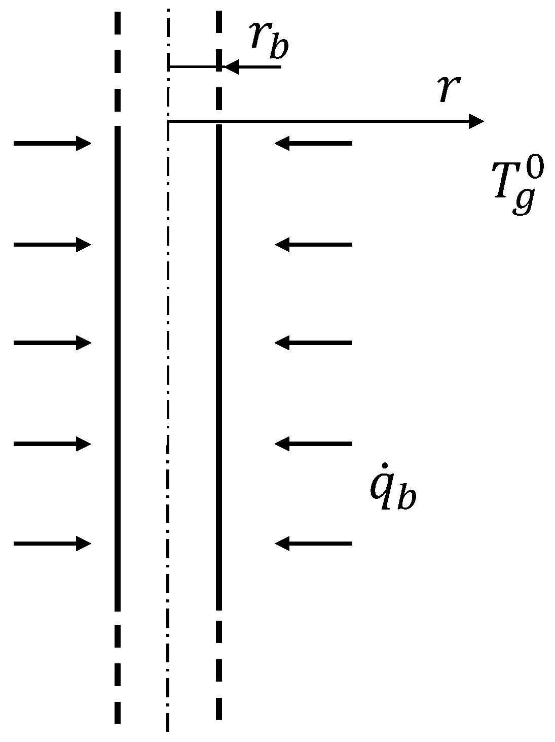
3. ICS—Infinite Cylindrical Source Model

This model represents the heat source as an infinitely long hollow cylinder embedded in a semi-infinite homogeneous medium with constant and isotropic properties (Figure 3). The heat flux q ˙ b is imposed at the surface ( r = r b ) . Similar to the ILS model, only the radial dimension is taken into account. In this case, the energy equation reads:
α g 2 T g r 2 + 1 r T g r = T g t T g r , t = T g 0 T g r , t = 0 = T g 0 q ˙ r b , t = 2 π r b λ g T g r | r = r b = q ˙ b
The dimensionless solution to the problem (5) is given in Equation (6) [23,26].
Θ g F o b , r r b = 1 π 2 0 exp β 2 F o b 1 J 1 2 ( β ) + Y 1 2 ( β ) J 0 r r b β Y 1 ( β ) + J 1 ( β ) Y 0 r r b β d β β 2
where J 0 and J 1 are Bessel functions of the first kind of order zero and one, respectively, Y 0 and Y 1 are Bessel functions of the second kind of order zero and one, respectively. The thermal field depends on two dimensionless groups: the Fourier number at the borehole radius, F o b = α g t / r b 2 , and the dimensionless radial distance, r r b .
Equation (6) can be hard to evaluate numerically. Ingersoll et al. [23] provides a table of reference values in the range 0.1 F o b 25.000 and r / r b = { 1 , 2 , 5 , 10 } . Another equivalent and handy expression of the ICS solution can be found in [24,29].
Figure 4 shows the dimensionless profile of Θ g evaluated through both the ILS and ICS expressions. We note that the deviation between the two models is negligible at sufficiently large F o b . Besides, increasing the r / r b value (i.e., increasing the distance from the heat source), the two models overlap at even smaller F o b . That means that the ICS model is more accurate only in the proximity of the ground heat exchanger or at small time scales. Ingersoll et al. [23] and Eskilson [22] state that the ICS model should be used only for F o r 20 and F o r 5 , respectively. Figure 4 shows also the graphical representation of the two above-mentioned criteria.
Ingersoll and Eskilson referred to the borehole surface (i.e., r / r b = 1 ); however, as shown in Figure 4, at larger radial coordinates, both criteria are too precautionary. Thus, we developed a novel correlation to find the maximum F o b beyond which the relative deviation between ICS and ILS models is lower than 5 % (see Figure 4). However, for r / r b 5 , the absolute deviation between the two models is so small that we can use the ILS model at any F o b .
For typical ground thermal diffusivities and BHE radii, Ingersoll and Eskilson criteria, at r / r b = 1 , correspond to a time period of about 1–7 days and 5–48 h, respectively. Depending on the r / r b value, the 5% deviation occurs in a time period of about 12 h to some days.

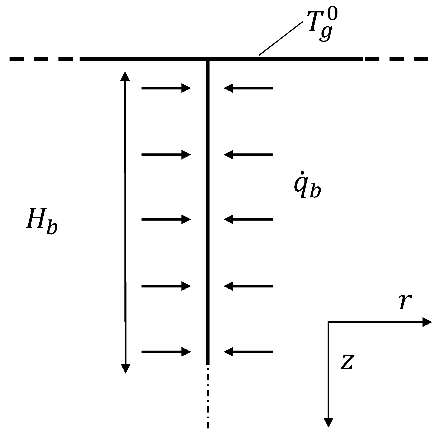
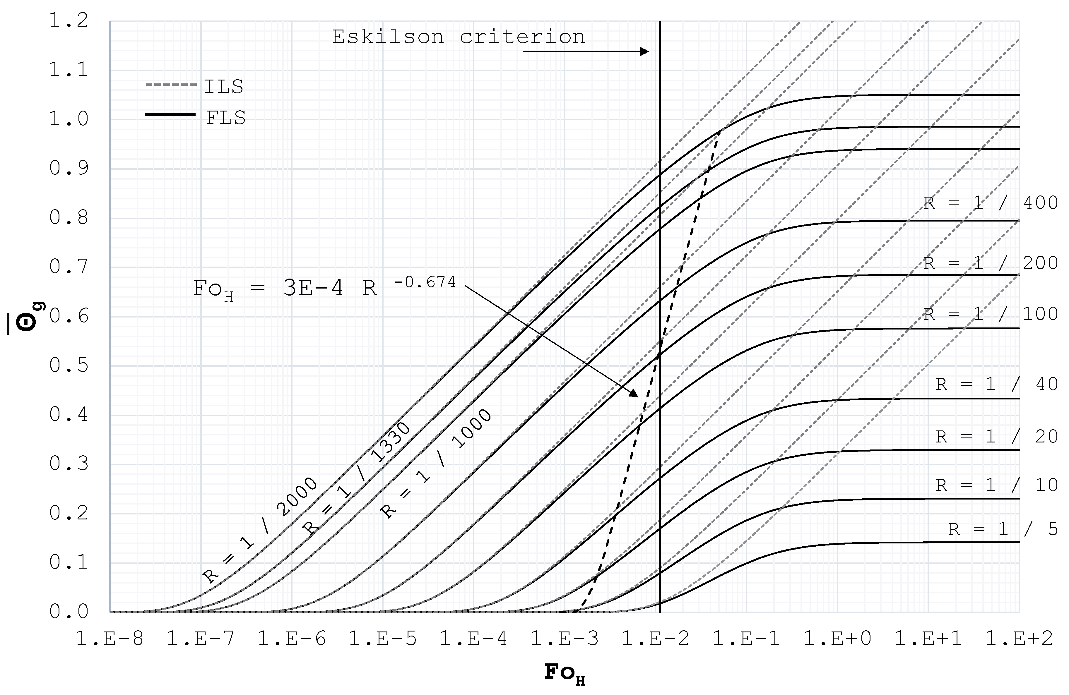
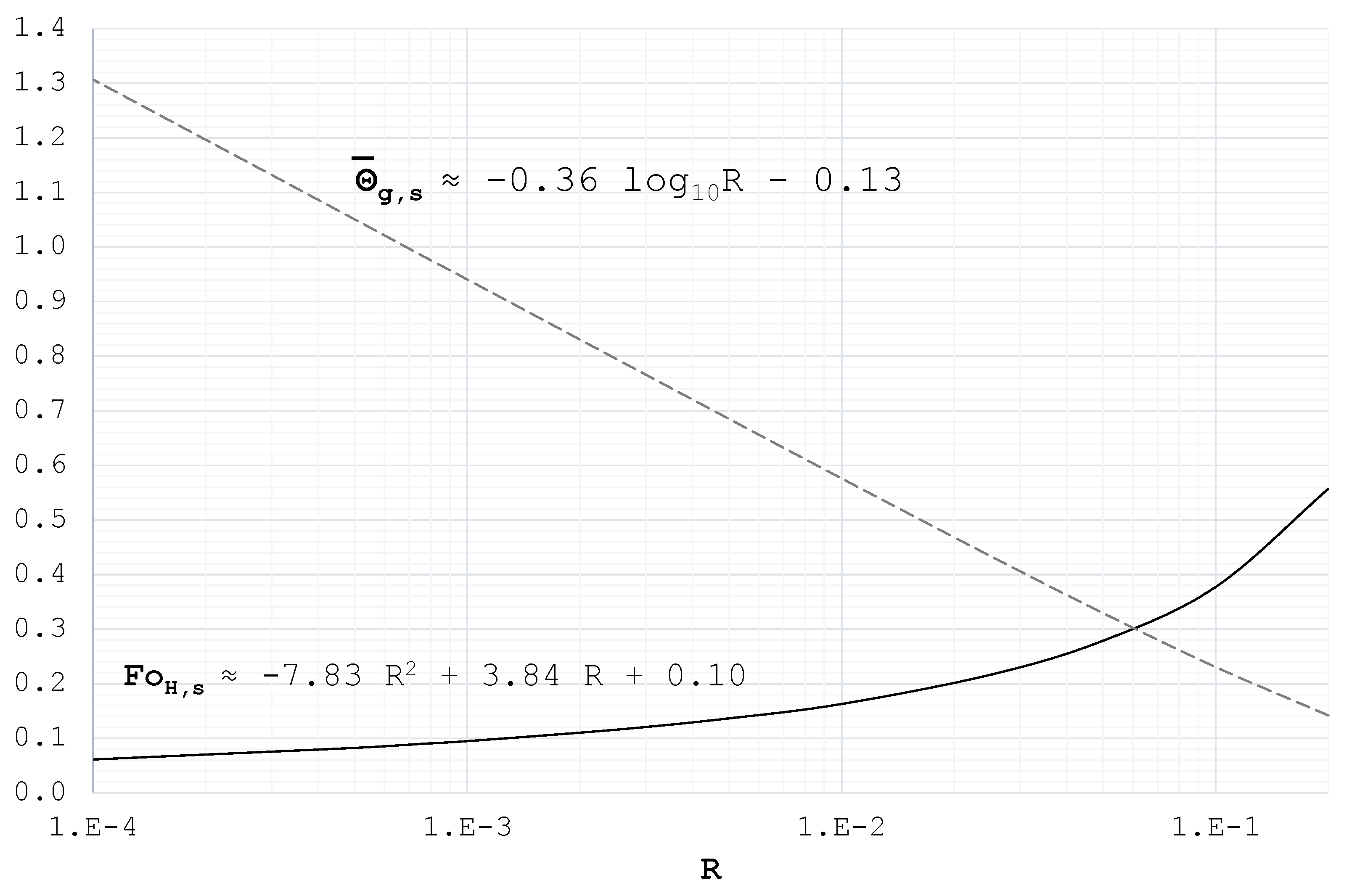
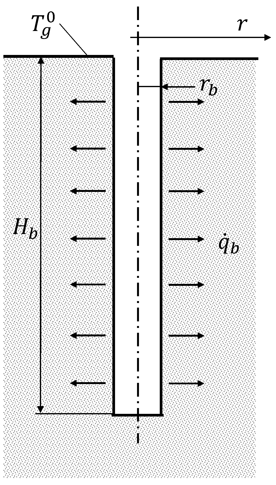
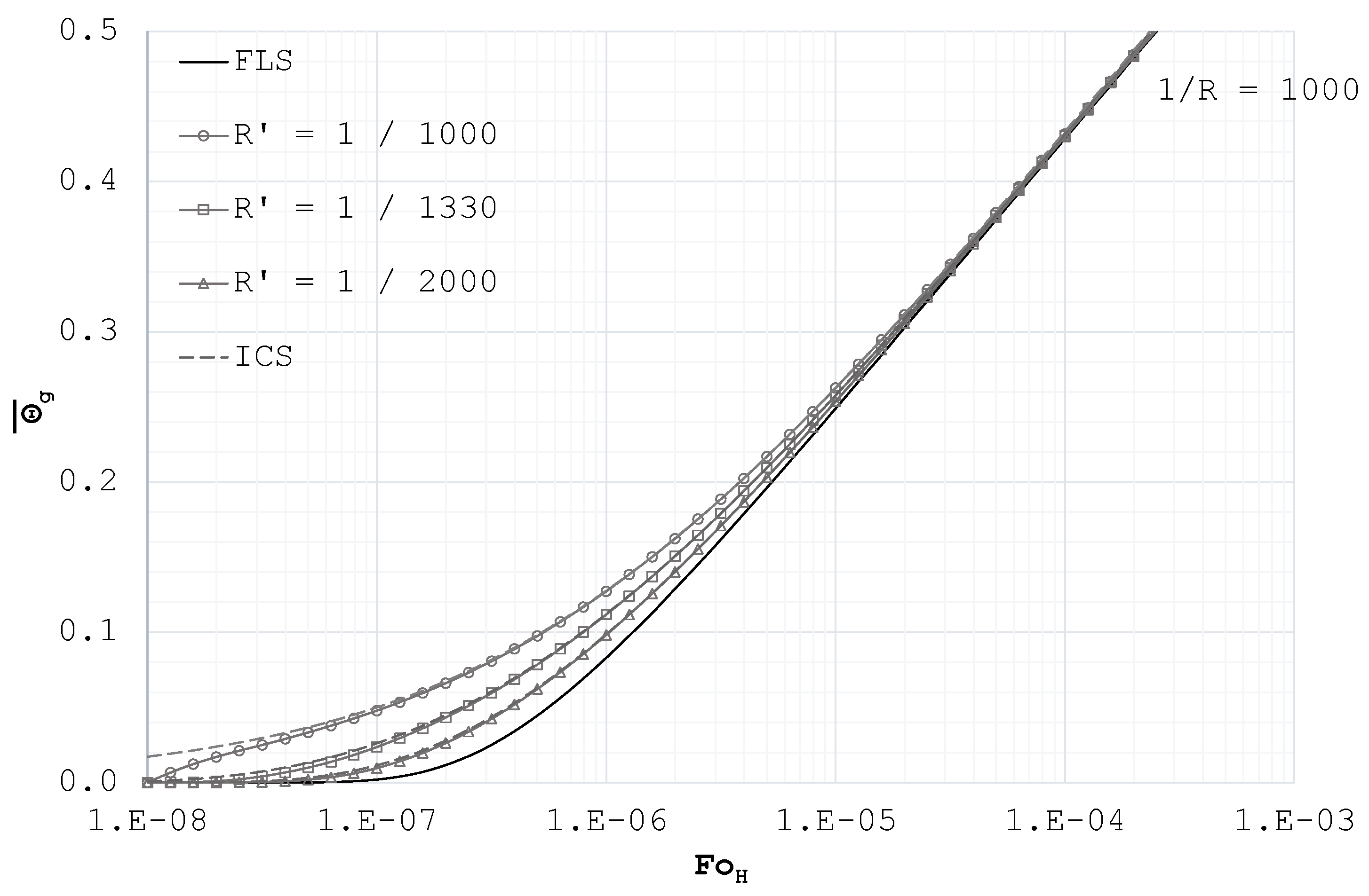
4. FLS—Finite Line Source Model

The FLS solution is able to consider the axial effects of the heat transfer process, occurring at long time scales [24]. The original formulation by Ingersoll et al. [22,23,26] has been improved in the last few decades by several authors (see, among others, [30,31,32]).
The FLS model is based on the following assumptions: the borehole is represented by a linear heat source of length H b with the top corresponding to the soil surface (see Figure 5); the ground is a semi-infinite homogeneous medium with constant and isotropic properties, and the soil surface is taken to be equal to T g 0 . It is worth recalling that the actual evolution of the surface temperature can be neglected below a depth of z > 3 α g ω , where ω is the main angular frequency of the surface temperature evolution [33]. This limit corresponds to a depth of about 5–8 m [22]; thus, for typical BHE depths, the actual evolution of the surface temperature does not significantly affect the heat transfer process. The validity of this assumption has to be verified for shallow systems (e.g., energy piles).
In the FLS model, the energy equation reads:
α g 2 T g r 2 + 1 r T g r + 2 T g z 2 = T g t T g r , z , t = T g 0 T g r , z , t = T g 0 T g r , z = 0 , t = T g 0 T g r , z , t = 0 = T g 0 q ˙ r , 0 z H b , t = 2 π r λ g T g r | r 0 = q ˙ b
The dimensionless solution of the FLS problem is [32]:
Θ g ( F o H , Z , R ) = 1 4 π 0 1 1 d / H b e r f c d / H b 2 F o H 1 d / H b e r f c d / H 2 F o H d Z
where:
F o H = α g t / H b 2 Z = z / H b R = r / H b Z = z / H b
d / H b = R 2 + ( Z Z ) 2 d / H b = R 2 + ( Z + Z ) 2
In engineering practice, it is convenient to have only one effective BHE temperature. Some authors take this reference value as the one at the middle depth ( z = H b / 2 ) ; others prefer the integral average temperature along the borehole depth. At long time scales, the former option overestimates the average temperature of the borehole surface (see, for instance, [24]); therefore, we always refer to the second alternative (Equation (9)).
Θ ¯ g = 0 1 Θ g d Z
Claesson and Javed [31] present a useful and fast expression to evaluate Θ ¯ g (see Equation (10)). Besides, they extend the generality of the FLS model by considering an arbitrary position of the line heat source, namely D < z < D + H b . Equation (8) refers to the case in which D = 0 .
Θ ¯ g = 1 4 π 1 / 4 F o H exp R 2 β 2 I l s β , D H b β β 2 d β
where:
I l s h , d = 2 · i e r f ( h ) + 2 · i e r f ( h + 2 d ) i e r f ( 2 h + 2 d ) i e r f ( 2 d ) i e r f ( x ) = 0 x e r f ( β ) d β = x · e r f ( x ) 1 π 1 exp x 2
Equation (10) introduces an additional dimensionless group with respect to Equation (8), i.e., D / H , that accounts for the depth of installation of the active part of the GHE. However, in this work, we analyze only the case in which D = 0 , in order to have a proper comparison with the other models.
Figure 6 shows the average dimensionless temperature, Θ ¯ g , as a function of the Fourier number, F o H , and dimensionless radial distance R = r / H b evaluated through the ILS and FLS solutions. As expected, the deviation between the two models becomes significant at large F o H values. The “Eskilson criterion” represents the classical limit for the applicability of the ILS solution as defined in [22], i.e., F o H = 1 / 90 . For typical ground thermal diffusivities and BHE depths, the Eskilson criterion corresponds to a large range of time of about 1–7 years. However, the just-mentioned criterion does not account for the actual evolution of the ground temperature at different radial distances, resulting in a relative deviation between FLS and ILS models that varies from about 15% down to 3% at large and small R values, respectively. On the contrary, Figure 6 provides also a more general criterion to assess the deviation between FLS and ILS models: the bold dashed lines represents the maximum F o H beyond which the relative deviation between the two models is higher than 5%.
In contrast with the ILS model, the FLS solution has a steady state value, “... although it may take a long time to reach this state” [23]. According to [23,24], Θ g , s reads:
Θ g , s ( Z , R ) = 1 4 π 0 1 1 d / H b 1 d / H b d Z
Figure 7 shows the value of Θ ¯ g , s depending on the R value and the Fourier number, F o H , s , corresponding to Θ ¯ g = 0.95 Θ ¯ g , s . As mentioned above, we need a very long period of time to reach the steady condition: e.g., for a typical BHE of a 100-m depth, the resulting F o H , s may even correspond to 250 years, depending on the soil thermal diffusivity.

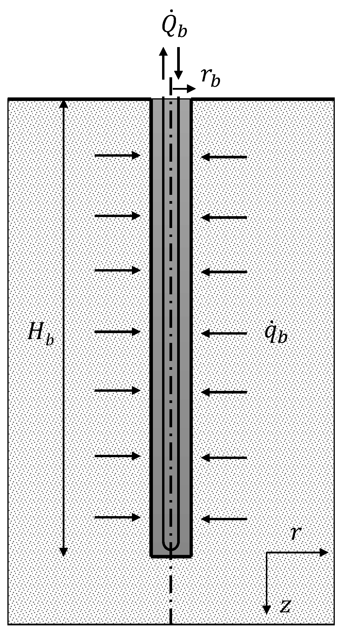
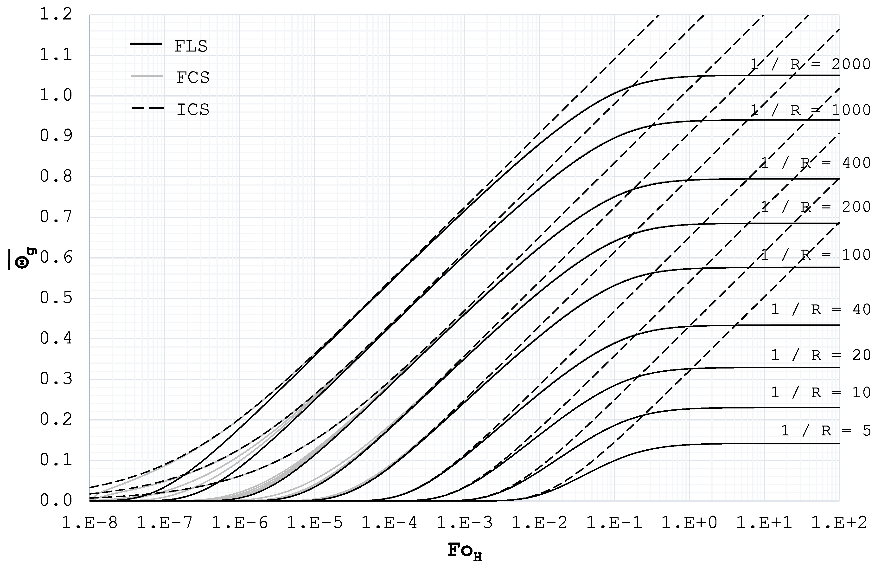
5. FCS—Finite Cylindrical Source Model

The FCS solution does not belong to the group of traditional analytical models (i.e., ILS, ICS and FLS). To our knowledge, the only available analytical expression of the FCS model was provided by Man et al. [28,32]. However, the proposed solution is based on a different geometry with respect to the above-described ICS model: specifically, the heat source is not assumed as a hollow cavity, but it consists of a cylindrical surface embedded in the soil domain. Man et al. named this model the “solid cylindrical source”, aiming at modeling those ground heat exchangers in which the internal material plays a significant role in the heat transfer process (e.g., energy piles).
In this work, we deal with the “hollow” finite cylindrical source; in other words, we refer to the geometry shown in Figure 8, where no material is considered within the heat generation surface. In this way, we provide a coherent comparison with the above-illustrated models, investigating possible improvements of the BHE modeling also in those cases where the grouting material can be assumed as a purely resistive body (i.e., when Equation (1) is applicable). The equations of the problem read:
α g 2 T g r 2 + 1 r T g r + 2 T g z 2 = T g t T g r , z , t = T g 0 T g r , z , t = T g 0 T g r , z = 0 , t = T g 0 T g r , z , t = 0 = T g 0 q ˙ r b , 0 z H b , t = 2 π r b λ g T g r | r = r b = q ˙ b
As mentioned above, an analytical solution of the problem (12) is not available in the literature. According to the dimensional analysis of the model, the FCS solution can be expressed through the following dimensionless groups:
Θ g = T g 0 T g λ g q ˙ b F o H = α g t / H b 2 Z = z / H b R = r / H b R = r b / H b
In this work, we derived the evolution of Θ g through a numerical FEM analysis using COMSOL Multiphysics® 5.2 [34]. The software was used for geometry design, meshing and the resolution of the transient heat conduction equation from zero to F o H = 10 2 . We used a 2D-axial symmetric domain with an unstructured triangular mesh. The axial and the radial extension of the domain was set equal to four-times the characteristic length of the problem (i.e., α g t ) in order to reproduce the behavior of a semi-infinite medium. The number of elements varies from about 20,000–90,000, depending on the dimension of the heat generation cavity. In particular, we performed a sensitivity analysis of the mesh dimension at the BHE wall: the resulting minimum element size to ensure the coherence between the imposed heat flux and the evaluated thermal gradient is equal to r b / 2 . The upper bound of the element size is 10 m. The simulation time stepping was based on the standard COMSOL BDF algorithm with a maximum step size corresponding to F o H = 1 . The standard COMSOL PARDISO solver was employed obtaining residuals always lower than 10−6.
We performed many numerical simulations by varying R in the range of the typical BHE values (see Figure 9). Similarly to the FLS model, we refer to the average value of Θ g between zero and H b (see Equation (9)); therefore, Z is not taken into account. The resulting Θ ¯ g profiles are shown in Figure 9.
Figure 10 compares the FCS and FLS models. It can be seen that, after a sufficient period of time, the FCS curves become equivalent to the FLS ones. Figure 11 shows in detail the case of 1 / R = 1000 : all of the lines at different R tend to the same FLS profile given by the specific R value.
It is possible to define a “critical” value, F o H , c , as a function of R and R, beyond which FCS and FLS models become practically equivalent. Here, we consider F o H , c as the Fourier number after which the relative difference between FCS and FLS models is less than 5% (see Figure 12).
The F o H , c value for a typical BHE with a depth of 100 m and a radius of 0.05 m, at the BHE surface (i.e., R / R = 1 ), corresponds to a few hours or days, depending on soil thermal diffusivity. At the typical distance between two BHEs, say 10 m (i.e., R / R = 200 ), F o H , c corresponds to a few months or years still depending on soil thermal diffusivity. However, we note that for R 100 , the actual deviation between the FCS and FLS models is practically negligible. This value corresponds to 0.5–1 m for typical boreholes; therefore, we can conclude that FLS model is sufficiently accurate at long time scales or to evaluating the thermal interference within a BHE field.
The FLS model can be used also to evaluate the FCS behavior at the steady state. In fact, as shown in Figure 10, for the typical aspect ratio of BHEs (i.e., 1 / 2000 R 1 / 400 ) and R values (i.e., 1 / 2000 R 1 / 5 ), F o H , c is lower than the corresponding F o H , s evaluated for the FLS model. Thus, we can extend Equation (11) and Figure 7 to the steady state of the FCS model.
With reference to the ICS model, we note a minor deviation with respect to the FCS profile only at low F o H (i.e., F o H 1 × 10 8 ) for R / R = 1 (see Figure 10 and Figure 11). This deviation becomes practically negligible at F o H 1 × 10 7 for any R and R . For typical BHEs, this time scale corresponds to a few hours; in other words, we are in the same order of magnitude of the lower temporal limit of the applicability of the “G-function”, t b . Therefore, for practical purposes, we can neglect this deviation. Regarding long time scales, as we discussed in Section 4, after a sufficiently long time period (see Figure 6), the ICS model behaves like the ILS one. Therefore, we can extend the same considerations about the FLS and ILS deviation also to ICS and FCS models (see Section 4) without further analyses.

6. Summary List of the Proposed Dimensionless Criteria

For the sake of readability, in this section, we present a short summary of the proposed deviation criteria among the ILS, ICS, FLS and FCS ground models. The reader may refer to the following list to chose readily the most appropriate model for his/her specific analysis. We recall that the term “practically equivalent” refers to a relative deviation lower than 5%.
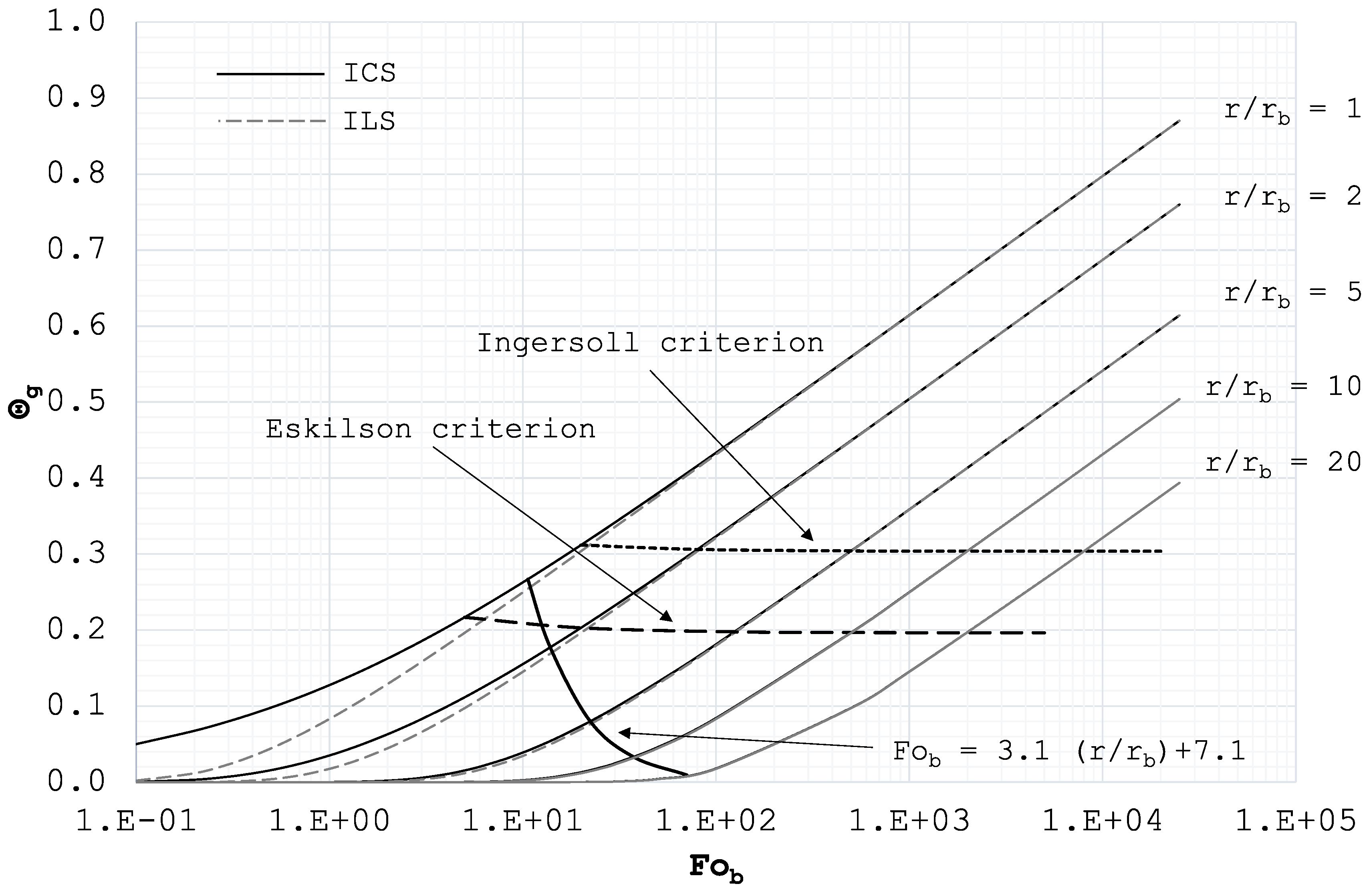
  • The ILS model is practically equivalent to the ICS one when:
    F o b 3.1 · ( r / r b ) + 7.1
  • The ILS model is practically equivalent to the FLS one when:
    F o H 3 × 10 4 · R 0.67
  • The ICS model is practically equivalent to the FCS one when:
    F o H 1 × 10 7
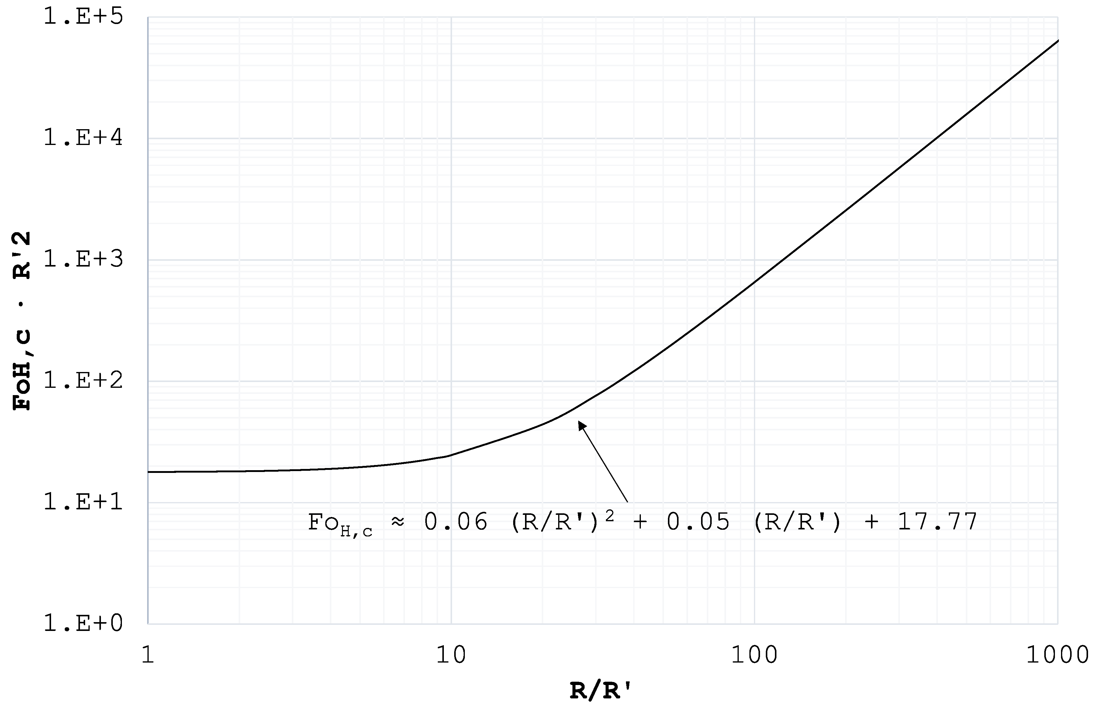
  • The FLS model is practically equivalent to the FCS one when:
    F o H 6.3 × 10 2 · ( R / R ) 2 + 5.4 × 10 2 · ( R / R ) + 17.8
Following the above list, the FLS model results in being the most suitable model for the thermal analysis of borehole heat exchangers. In fact, it can be successfully applied in a wide range of time and space scales, practically providing the same or better results than the other models.

7. Superposition Techniques

All of the above-described analytical models refer to the ground response when a constant heat pulse is imposed at a single borehole surface. The operative conditions of real GSHPs are different: first, a typical BHE field is made of several boreholes, any of which exchanges a time-variable thermal power. The actual evolution of the heat flux q ˙ b depends on several factors: e.g., building thermal load profile, instantaneous COP/EER of the heat pump unit, heat transfer effectiveness of each borehole, supply temperature and the instantaneous value of the ground temperature resulting from previous heat exchanges. Only a complete simulation model, taking into account the behavior of each GSHP subsystem, is able to evaluate the actual heat flux at each borehole surface [3].
In this section, we describe the mathematical techniques to obtain the analytical expression of the ground temperature when more than one time-dependent heat source is considered, i.e., the time superposition and space superposition techniques.

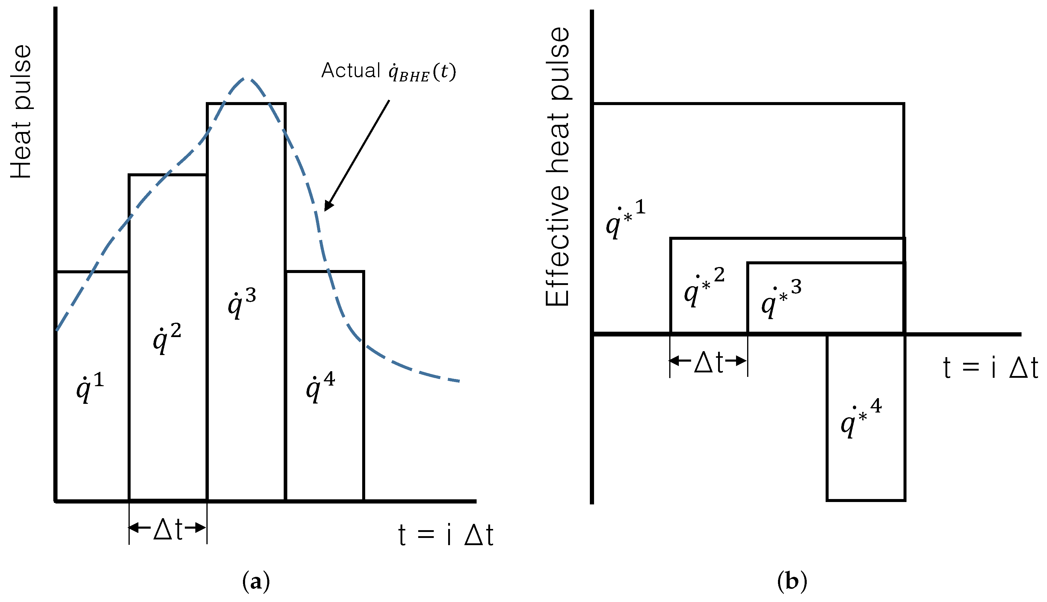
7.1. Time Superposition Technique

The solution to heat transfer problems with time-dependent boundary conditions can be related to the solution of the same problem with constant boundary conditions by means of the Duhamel’s theorem [33]. In other words, we evaluate the ground temperature response to an arbitrary time-dependent q ˙ b ( t ) through the “fundamental solution” of the same problem to a single, constant, unitary heat pulse.
All of the Θ g ( x , t ) expressions illustrated in the previous sections (i.e., the ILS, FLS, ICS and FCS models) are fundamental solutions. Therefore, according to Duhamel’s theorem, the ground response to a time-varying term q ˙ b ( t ) reads:
T g ( x , t ) T g 0 λ g = 0 t Θ g ( x , t β ) q ˙ b d t ( β ) d β + Θ g ( x , 0 ) · q ˙ B H E ( 0 )
where x is the generic spatial coordinate, β is the auxiliary time variable, and Θ g corresponds to Equations (3), (6) and (8) or Figure 9, depending on the employed model.
For practical purposes, the GSHP analysis is typically based on a quasi steady-state formulation [3]: in other words, the actual evolution of the physical quantities (e.g., temperature and energy exchanges) is approximated by a series of constant average values (see Figure 13a). Thus, the general expression of Duhamel’s theorem (Equation (13)) can be modified as follows:
T g ( x , t = n Δ t ) T g 0 λ g = i = 1 n Θ g ( x , t = i Δ t ) q ˙ b n i + 1 q ˙ b n i
where T g ( x , t = n Δ t ) corresponds to the ground temperature at the end of the n-th time step and q ˙ b 0 = 0 .
The physical interpretation of Equation (14) is shown in Figure 13b. The basic heat pulse q ˙ b 1 is applied for the entire duration of the analysis (four time steps in Figure 13b). Successively, we superimpose other “effective pulses”, namely: q ˙ 2 = q ˙ b 2 q ˙ b 1 for three time steps, q ˙ 3 = q ˙ b 3 q ˙ b 2 for two time steps and q ˙ 4 = q ˙ b 4 q ˙ b 3 for the last step.

7.2. Space Superposition Technique

If we assume that the radial dimension of each BHE is negligible with respect to the size of the field, the ground temperature at a given coordinate x is obtained by summing up all of the individual temperature alterations caused by each borehole, namely:
Θ g ( x , t ) = j = 1 N b Θ g , j x x j , t
where N b is the boreholes number and x b is the position of the j-th borehole.
Considering both time and space superposition, the final expression of the ground thermal field reads:
T g ( x , t = n Δ t ) = T g 0 j = 1 N b i = 1 n Θ g x x j , t = i Δ t λ g q ˙ b , j n i + 1 q ˙ b , j n i

8. Illustrative Examples

In this section, we propose two brief application examples of the proposed expressions and maps: the first one compares the above-described models in order to show the coherence between the numerical results and the above-mentioned considerations; the second example shows how the proposed charts can be conveniently and successfully used to evaluate the necessary spacing and avoid the thermal interference between two BHEs.

8.1. Example #1

In this first example, we compare the deviation among the ILS, ICS, FLS and FCS models in terms of ground temperature evaluation. Specifically, we analyze the relevance of the axial dimension (finite depth models) and the actual BHE radius (cylindrical models). We refer to two configurations, whose parameters are presented in Table 2. The configurations have the same BHE radius, r b , but different H b : the first one has a greater depth (low aspect ratio, R ) with respect to the others. The thermal evolution of the ground source is evaluated at six different time scales (i.e., after one day, one week, one month, one, five and ten years) and at three different radial position (i.e., on the BHE wall, 5 m and 10 m away from the BHE axis) in order to analyze both the thermal behavior of the borehole and its interference with adjacent ground heat exchangers. Different radial positions allow also the evaluation of the relevance of axial dimension at different time scales. Table 3 and Table 4 summarize all of the results for the two above-mentioned configurations.
With regard to the cylindrical models, as predicted by Figure 4 and Figure 10, we note that in the two configurations, both ICS and FCS models deviate from ILS and FLS models only at short time scales (i.e., daily period) and R / R = 1 . No significant effects occur at greater radial distances. As expected, the axial dimension becomes significant only at long time scales in accordance with the criteria in Figure 4 and Figure 12. The higher the aspect ratio R , the higher the deviation among infinite and finite models.

8.2. Example #2

In this second example, we show how the proposed maps can be conveniently and successfully used to properly size a BHEs field according to the specific thermal load and ground thermo-physical properties.
Suppose that we want to determine the minimum distance between two BHEs (say, A and B) in order to avoid the thermal interference among them. We choose a a temperature increase of 0.5 K as the maximum alteration that A can produce on B, and vice versa. The thermal load can be assumed as constant and equal to q ˙ b = 35 W·m−1. The period to be taken into account is four months. The ground thermo-physical properties and BHEs geometrical characteristics are shown in Table 2.
According to the above-mentioned parameters, we want to maintain the dimensionless temperature Θ ¯ g lower than 0.5 × 1.5 35 = 0.02 . The F o H corresponding to four mounts (i.e., 120 days) is 5 × 10⁻⁴. We can use these two values as coordinates in the FLS map (Figure 6), obtaining the dimensionless radial distance R = 1 / 20 . This value corresponds to 5 m for a 100- m BHE depth. Obviously, the just-described procedure does not represent an actual and complete design strategy, but we showed how the proposed maps can be used for quick preliminary or verification analyses.

9. Conclusions

In this work, we dealt with several analytical models for the ground source in the GSHP context. Specifically, we reviewed and discussed the traditional infinite, finite, linear and cylindrical models for borehole heat exchangers. Besides, we developed the “hollow” finite cylindrical source model that was still missing in the scientific literature. After a brief discussion of the assumptions and the characteristics of each model, we performed some dimensionless analyses of the evolution of the ground thermal field in order to figure out some universal and general criteria to decide which model should be employed in any specific case. These criteria are summarized in Section 6.
In conclusion, FLS seems to be the most suitable model both for BHE design and multi-year operative analyses. The ILS model tends to overestimate the temperature level of the ground source, especially at high values of the dimensionless distance from the borehole (i.e., R / R ). Cylindrical models are particularly suitable to investigate the temperature evolution near the ground heat exchanger at short time scales, but, for the typical analyses in the GSHP context, we deal with time and space scales in which both ICS and ILS models are practically equivalent to the ILS and FLS ones, respectively. Moreover, it is worth recalling that all of the analyzed models can be applied only for times longer than t b (generally a few hours), while they are not able to predict very short-time responses that are related to the transient behavior of the ground heat exchanger. For typical BHE geometries, the time scale beyond which the cylindrical models deviate from the linear ones is very close to t b , making ICS and FCS models ineffective. In short, the FLS model represents a proper tradeoff between modeling accuracy and computational effort for all of the typical BHE design and simulation contexts.
In this work, we do not consider groundwater movement. Future works will be aimed at finding similar dimensionless criteria to evaluate in which time and space scales the fluid advection significantly affects the thermal response of the ground source. In other words, we will develop a quantitative relationship between the Fourier and the Péclet numbers to assess when purely-conductive molds have to be replaced by the “porous media” theory. Besides, we will extend our analysis to other ground heat exchangers, e.g., horizontal configurations and shallow heat exchangers, such as energy piles or baskets.

Acknowledgments

The author gratefully acknowledges the University of Pisa for the ongoing funding PRA 2016 on energy system integration, which supported the research. Thanks also to the other members of the BETTER group who assisted the preparation of this paper. A particular mention goes to Walter Grassi and Daniele Testi for their suggestions and comments that greatly improved the manuscript.

Conflicts of Interest

The authors declare no conflict of interest.

Nomenclature

Acronyms 

ASHRAE
American Society of Heating, Refrigerating and Air-Conditioning Engineers
BHE
Borehole heat exchanger
COP
Coefficient of performance of the heat pump in heating mode
EER
Coefficient of performance of the heat pump in cooling mode
FCS
Finite cylindrical source model
FLS
Finite line source model
GHE
Ground heat exchanger
GSHP
Ground-source heat pump system
ICS
Infinite cylindrical source model
ILS
Infinite line source model

Symbols 

D
BHE installation depth
E i
Exponential integral function
F o r
Fourier number referred to the radial coordinate
F o b
Fourier number referred to the borehole radius
F o H
Fourier number referred to the borehole depth
G
“G-function” or dimensionless soil temperature
H b
Borehole depth, m
N b
Boreholes number
Q ˙
Thermal power, W
R
Dimensionless radial coordinate
R
BHE aspect ratio
R b
Borehole thermal resistance, m·K·W−1
T
Temperature, K or °C
Z
Dimensionless axial coordinate
e r f
Gauss error function
q ˙
Linear heat flux, W·m−1
r
Radius, m
r b
Borehole radius, m
t
Time, s
t b
Borehole characteristic time, s
x
Position vector, m
z
Axial coordinate, m

Greek Letters 

α
Thermal diffusivity, m2·s−1
β
Auxiliary integration variable
λ
Thermal conductivity, W·m−1·K−1
γ
Euler’s constant
Θ
Dimensionless temperature

Subscripts 

b
Borehole
g
Ground source
f
Circulating fluid within BHE ducts
s
Steady state

Superscripts 

¯
Mean value
0
Initial time
n
Current time step
i
Generic time step

References

  1. Sarbu, I.; Sebarchievici, C. General review of ground-source heat pump systems for heating and cooling of buildings. Energy Build. 2014, 70, 441–454. [Google Scholar] [CrossRef]
  2. Carvalho, A.D.; Moura, P.; Vaz, G.C.; de Almeida, A.T. Ground source heat pumps as high efficient solutions for building space conditioning and for integration in smart grids. Energy Convers. Manag. 2015, 103, 991–1007. [Google Scholar] [CrossRef]
  3. Grassi, W.; Conti, P.; Schito, E.; Testi, D. On sustainable and efficient design of ground-source heat pump systems. J. Phys. Conf. Ser. 2015, 655, 012003. [Google Scholar] [CrossRef]
  4. Conti, P. A novel evaluation criterion for GSHP systems based on operative performances. In Proceedings of the 2015 5th International Youth Conference on Energy (IYCE), Pisa, Italy, 27–30 May 2015; pp. 1–8.
  5. Atam, E.; Helsen, L. Ground-coupled heat pumps: Part 1—Literature review and research challenges in modeling and optimal control. Renew. Sustain. Energy Rev. 2015, 54, 1653–1667. [Google Scholar] [CrossRef]
  6. Atam, E.; Helsen, L. Ground-coupled heat pumps: Part 2—Literature review and research challenges in optimal design. Renew. Sustain. Energy Rev. 2015, 54, 1668–1684. [Google Scholar] [CrossRef]
  7. Robert, F.; Gosselin, L. New methodology to design ground coupled heat pump systems based on total cost minimization. Appl. Therm. Eng. 2014, 62, 481–491. [Google Scholar] [CrossRef]
  8. Comparison, J.D.S.; Cullin, J.R.; Spitler, J.D. Comparison of simulation-based design procedures for hybrid ground source heat pump systems. In Proceedings of the 8th International Conference on System Simulation in Buildings, Liege, Belgium, 13–15 December 2010.
  9. Sayyaadi, H.; Amlashi, E.H.; Amidpour, M. Multi-objective optimization of a vertical ground source heat pump using evolutionary algorithm. Energy Convers. Manag. 2009, 50, 2035–2046. [Google Scholar] [CrossRef]
  10. Alavy, M.; Nguyen, H.V.; Leong, W.H.; Dworkin, S.B. A methodology and computerized approach for optimizing hybrid ground source heat pump system design. Renew. Energy 2013, 57, 404–412. [Google Scholar] [CrossRef]
  11. Nguyen, A.T.; Reiter, S.; Rigo, P. A review on simulation-based optimization methods applied to building performance analysis. Appl. Energy 2014, 113, 1043–1058. [Google Scholar] [CrossRef]
  12. Casarosa, C.; Conti, P.; Franco, A.; Grassi, W.; Testi, D. Analysis of thermodynamic losses in ground source heat pumps and their influence on overall system performance. J. Phys. Confer. Ser. 2014, 547, 012006. [Google Scholar] [CrossRef]
  13. Al-Khoury, R. Computational Modeling of Shallow Geothermal Systems; CRC Press: Boca Raton, FL, USA, 2012; Volume 4, p. 245. [Google Scholar]
  14. Kim, E.J.; Roux, J.J.; Bernier, M.A.; Cauret, O. Three-dimensional numerical modeling of vertical ground heat exchangers: Domain decomposition and state model reduction. HVAC R Res. 2011, 17, 912–927. [Google Scholar]
  15. Conti, P.; Testi, D.; Grassi, W. Revised heat transfer modeling of double-U vertical ground-coupled heat exchangers. Appl. Therm. Eng. 2016, 106, 1257–1267. [Google Scholar] [CrossRef]
  16. Batini, N.; Rotta Loria, A.F.; Conti, P.; Testi, D.; Grassi, W.; Laloui, L. Energy and geotechnical behaviour of energy piles for different design solutions. Appl. Therm. Eng. 2015, 86, 199–213. [Google Scholar] [CrossRef]
  17. Vaccaro, M.; Conti, P. Numerical simulation of geothermal resources: A critical overlook. In Proceedings of the European Geothermal Congress 2013, Pisa, Italy, 3–7 June 2013.
  18. Lamarche, L. Short-term behavior of classical analytic solutions for the design of ground-source heat pumps. Renew. Energy 2013, 57, 171–180. [Google Scholar] [CrossRef]
  19. Geothermal Energy. In ASHRAE Handbook—HVAC Applications; American Society of Heating, Refrigerating and Air-Conditioning Engineers (ASHRAE): Atlanta, GA, USA, 2011; Chapter 34; p. 34.
  20. Colangelo, G.; Romano, D.; de Risi, A.; Starace, G.; Laforgia, D. A Matlab-Simulink tool for ground source heat pumps simulation. La Termotec. 2012, 3, 63–72. (In Italian) [Google Scholar]
  21. Li, M.; Lai, A.C. Review of analytical models for heat transfer by vertical ground heat exchangers (GHEs): A perspective of time and space scales. Appl. Energy 2015, 151, 178–191. [Google Scholar] [CrossRef]
  22. Eskilson, P. Thermal Analysis of Heat Extraction Boreholes. Ph.D. Thesis, University of Lund, Lund, Sweden, 1987. [Google Scholar]
  23. Ingersoll, L.R.; Zobel, O.J.; Ingersoll, A.C. Heat Conduction with Engineering, Geological and Other Applications; McGraw-Hill: New York, NY, USA, 1954; p. 325. [Google Scholar]
  24. Philippe, M.; Bernier, M.; Marchio, D. Validity ranges of three analytical solutions to heat transfer in the vicinity of single boreholes. Geothermics 2009, 38, 407–413. [Google Scholar] [CrossRef]
  25. Kelvin, T.W. Mathematical and Physical Papers; Cambridge University Press: London, UK, 1882. [Google Scholar]
  26. Carslaw, H.S.; Jeager, J.C. Conduction of Heat in Solids, 2nd ed.; Clarendon Press: Oxford, UK, 1959. [Google Scholar]
  27. Kavanaugh, S.P.; Rafferty, K. Design of Geothermal Systems for Commercial and Institutional Buildings; American Society of Heating, Refrigerating and Air-Conditioning Engineers (ASHRAE): Atlanta, GA, USA, 1997; p. 167. [Google Scholar]
  28. Man, Y.; Yang, H.; Diao, N.; Liu, J.; Fang, Z. A new model and analytical solutions for borehole and pile ground heat exchangers. Int. J. Heat Mass Transf. 2010, 53, 2593–2601. [Google Scholar] [CrossRef]
  29. Baudoin, A. Stockage Intersaisonnier de Chaleur Dans le sol par Batterie D’échangeurs Baionnette Verticaux: Modèle de préDimensionnement. Ph.D. Thesis, Université de Reims Champagne-Ardenne, Reims, France, 1988. [Google Scholar]
  30. Zeng, H.Y.; Diao, N.R.; Fang, Z.H. A finite line-source model for boreholes in geothermal heat exchangers. Heat Transf. Asian Res. 2002, 31, 558–567. [Google Scholar] [CrossRef]
  31. Claesson, J.; Javed, S. An analytical method to calculate borehole fluid temperatures for time-scales from minutes to decades. ASHRAE Trans. 2011, 117, 279–288. [Google Scholar]
  32. Li, M.; Lai, A.C. Heat-source solutions to heat conduction in anisotropic media with application to pile and borehole ground heat exchangers. Appl. Energy 2012, 96, 451–458. [Google Scholar] [CrossRef]
  33. Ozisik, M.N. Heat Conduction; John Wiley & Sons: Hoboken, NJ, USA, 1993. [Google Scholar]
  34. COMSOL Multiphysics® v. 5.2. COMSOL AB. Available online: http//:www.comsol.com (accessed on 26 October 2016).
Figure 1. Schematic diagram of a typical borehole heat exchanger.
Energies 09 00890 g001
Figure 2. Schematic representation of the infinite line source model.
Energies 09 00890 g002
Figure 3. Schematic representation of the infinite cylindrical source model.
Energies 09 00890 g003
Figure 4. Dimensionless temperature, Θ g , given by the ILS (gray lines) and ICS models (black lines). The expression F o b 3.1 r / r b + 7.1 evaluates the maximum F o b beyond which the relative deviation between ICS and ILS models is lower than 5 %.
Energies 09 00890 g004
Figure 5. Schematic representation of a finite line heat source model. The surface temperature is fixed to T g 0 .
Energies 09 00890 g005
Figure 6. FLS solution: the average dimensionless temperature, Θ ¯ g , evaluated through the FLS model (solid lines) and the ILS model (dashed lines). The bold vertical line represents the Eskilson criterion, i.e., F o H = 1 / 90 . The bold dashed line represents the limit beyond which the relative deviation between FLS and ILS models is higher than 5%.
Energies 09 00890 g006
Figure 7. FLS model: steady state Θ ¯ g , s and F o H , s as a function of R.
Energies 09 00890 g007
Figure 8. Schematic representation of the “hollow” finite cylindrical source model.
Energies 09 00890 g008
Figure 9. Dimensionless temperature, Θ ¯ g , as a function of F o H , BHE aspect ratio, R = r b / H b , and dimensionless radial distance from the BHE, R / R = r / r b . (a) R = 1 / 2000 ; (b) R = 1 / 1330 ; (c) R = 1 / 1000 ; (d) R = 1 / 800 ; (e) 1/400.
Energies 09 00890 g009
Figure 10. Dimensionless temperature Θ g evaluated through the FCS (black lines), FLS (gray lines) and ICS models at different R = r / H b and R = r b / H b values.
Energies 09 00890 g010
Figure 11. Dimensionless temperature Θ g evaluated through the FCS and FLS models for R = r / H b = 1 / 1000 .
Energies 09 00890 g011
Figure 12. F o H , c as a function of R and R . F o H , c corresponds to the time after which the relative difference between the FCS and FLS models is less than 5%.
Energies 09 00890 g012
Figure 13. Superposition of piecewise heat steps. The actual pulses q ˙ 1 , q ˙ 2 , q ˙ 3 , q ˙ 4 are superimposed in time as “effective pulses” q ˙ 1 , q ˙ 2 , q ˙ 3 , q ˙ 4 . (a) Actual thermal pulses; (b) effective thermal pulses.
Energies 09 00890 g013
Table 1. Classification scheme and acronyms for analytical ground heat transfer models in GSHP.
GeometryPurely-Conductive MediaSaturated Porous Media
Infinite axial extensionILS
Infinite line source
ICS
Infinite cylindrical source
MILS
Moving infinite line source
MICS
Moving infinite cylindrical source (not yet developed)
Finite axial extensionFLS
Finite line source
FCS
Finite cylindrical source
MFLS
Moving finite line source
MFCS
Moving finite cylindrical source (not yet developed)
Table 2. Parameters for the two analyzed configurations.
ParameterConfiguration #1Configuration #2
Ground thermal conductivity, λ g W·m−1·K−11.51.5
Ground thermal diffusivity, α g m2·s−14.8 × 10−74.8 × 10−7
Borehole radius, r b m0.0750.075
Borehole depth, H b m10060
Table 3. Configuration #1: comparison among the Θ ¯ g values evaluated through different analytical models. r b = 0.075 m , H b = 100 m , R = 1 / 1330 .
r0.075510
t1 Day1 Week1 Month1 Year5 Years10 Years1 Day1 Week1 Month1 Year5 Years10 Years1 Day1 Week1 Month1 Year5 Years10 Years
F o r 7.4 × 10 0 5.2 × 10 1 2.2 × 10 2 2.7 × 10 3 1.3 × 10 4 2.7 × 10 4 1.7 × 10 3 1.2 × 10 2 5.0 × 10 2 6.1 × 10 1 3.0 × 10 0 6.1 × 10 0 4.2 × 10 4 2.9 × 10 3 1.2 × 10 2 1.5 × 10 1 7.6 × 10 1 1.5 × 10 0
F o H 6.9 × 10 6 4.8 × 10 5 2.1 × 10 4 2.5 × 10 3 1.3 × 10 2 2.5 × 10 2 6.9 × 10 6 4.8 × 10 5 2.1 × 10 4 2.5 × 10 3 1.3 × 10 2 2.5 × 10 2 6.9 × 10 6 4.8 × 10 5 2.1 × 10 4 2.5 × 10 3 1.3 × 10 2 2.5 × 10 2
ILS0.230.380.490.690.820.880.000.000.000.050.160.210.000.000.000.010.070.11
ICS0.240.380.500.690.820.880.000.000.000.050.160.210.000.000.000.010.070.11
FLS0.230.380.490.680.800.840.000.000.000.050.150.190.000.000.000.010.060.10
FCS0.340.380.490.680.800.840.000.000.000.050.150.190.000.000.000.010.060.10
Table 4. Configuration #2: comparison among the Θ ¯ g values evaluated through different analytical models. r b = 0.075 m , H b = 60 m , R = 1 / 800 .
r0.075510
t1 Day1 Week1 Month1 Year5 Years10 Years1 Day1 Week1 Month1 Year5 Years10 Years1 Day1 Week1 Month1 Year5 Years10 Years
F o r 7.4 × 10 0 5.2 × 10 1 2.2 × 10 2 2.7 × 10 3 1.3 × 10 4 2.7 × 10 4 1.7 × 10 3 1.2 × 10 2 5.0 × 10 2 6.1 × 10 1 3.0 × 10 0 6.1 × 10 0 4.2 × 10 4 2.9 × 10 3 1.2 × 10 2 1.5 × 10 1 7.6 × 10 1 1.5 × 10 0
F o H 1.2 × 10 5 8.1 × 10 5 3.5 × 10 4 4.2 × 10 3 2.1 × 10 2 4.2 × 10 2 1.2 × 10 5 8.1 × 10 5 3.5 × 10 4 4.2 × 10 3 2.1 × 10 2 4.2 × 10 2 1.2 × 10 5 8.1 × 10 5 3.5 × 10 4 4.2 × 10 3 2.1 × 10 2 4.2 × 10 2
ILS0.230.380.490.690.820.880.000.000.000.050.160.210.000.000.000.010.070.11
ICS0.240.380.500.690.820.880.000.000.000.050.160.210.000.000.000.010.070.11
FLS0.230.380.490.680.780.820.000.000.000.050.140.170.000.000.000.010.060.09
FCS0.370.380.490.680.780.820.000.000.050.050.140.170.000.000.000.010.060.09

