Definition and Experimental Validation of a Simplified Model for a Microgrid Thermal Network and its Integration into Energy Management Systems

Abstract

The present paper aims at defining a simplified but effective model of a thermal network that links the thermal power generation with the resulting temperature time profile in a heated or refrigerated environment. For this purpose, an equivalent electric circuit is proposed together with an experimental procedure to evaluate its input parameters. The paper also highlights the simplicity of implementation of the proposed model into a microgrid Energy Management System. This allows the optimal operation of the thermal network to be achieved on the basis of available data (desired temperature profile) instead of a less realistic basis (such as the desired thermal power profile). The validation of the proposed model is performed on the Savona Campus Smart Polygeneration Microgrid (SPM) with the following steps: (i) identification of the parameters involved in the equivalent circuit (performed by minimizing the difference between the temperature profile, as calculated with the proposed model, and the measured one in a set of training days); (ii) test of the model accuracy on a set of testing days (comparing the measured temperature profiles with the calculated ones); (iii) implementation of the model into an Energy Management System in order to optimize the thermal generation starting from a desired temperature hourly profile.

1. Introduction

One of the main focuses of microgrid research has been the development of optimal operational strategies to reach the maximum potential of their promising features in the energy management context. Such strategies are typically implemented in so-called Energy Management Systems (EMS).

Due to their importance, EMSs have been deeply investigated in various forms and architectures [1,2]. The most common architecture for EMSs is the multilevel hierarchical architecture [3], in which the higher level accounts for the dispatch of active and reactive power of the programmable production units, while the lower ones perform a more detailed control of the single units. The highest level of this architecture recalls the principles of optimization of traditional electricity transmission networks, achieved by classical Optimal Power Flow (OPF) algorithms. However, the presence of dynamic components such as storage devices, together with the uncertainties that characterize load request and renewable energy sources (RES), and the combined presence of electric and thermal infrastructure make this optimization problem a very hard task from a computational point of view. To overcome this difficulty, many different papers have been published with the aim of developing accurate and efficient algorithms for microgrid EMSs, addressing either the integration of RES and storage devices, the so-called demand side management (DSM), or again the satisfaction of electric network constraints [4,5,6].

In a recent paper [7], the attention of the authors has been concentrated on efficient electric network modeling for optimization purposes that has reached a good compromise between accuracy and reduction in the Computer Processing Unit (CPU) effort. However, the thermal network model consisted only of a pure thermal power balance equation. This is quite unrealistic, as it assumes knowledge of the current and future thermal load request expressed in terms of a thermal power rather than a temperature profile and does not consider the dynamic transients between the instant in which the thermal source is switched on and the moment in which the temperature reaches the desired value. The proposed paper aims at bridging this gap by defining an equivalent electric circuit for a thermal network that is able to account for both these issues.

In the literature, many studies have dealt with the modeling of thermal networks from different point of views (as an example [8,9,10]) focusing either on optimization or simulation aspects. The advantages of district heating networks based on combined heating and power (CHP) technologies have been shown in [11,12] and, especially in [11], a model for the optimal daily operation of a district system with a CHP plant has been proposed.

As highlighted by Larsen et al. [13], models including a full physical representation of thermal networks, in terms of mass flow rates, pressure drops and pipe dimensions, are computationally intensive and, as a consequence, are not suitable to be inserted into EMSs; to this end, they propose a simplified method which permits them to study a district heating network by reducing its topological complexity. On the other hand, Kuosa et al. [14] focus their attention on the differences between radial and meshed networks and compare a traditional network with a ring one characterized by an innovative flow rate control method. Furthermore, the same authors introduced in [8] an equivalent thermal circuit to represent the heat transfer process in a heat exchanger and applied this methodology to study a district heating system.

More simplified models of thermal networks are usually implemented within Mixed-Integer Linear Programming (MILP) tools [15,16,17], where district heating networks are optimally designed and operated in order to minimize different objectives, such as capital and daily operational costs. In the aforementioned models, energy balance equations, operational constraints and correlations for the calculation of heat losses and pressure drops are reported. In any case, what is necessary for an EMS is basically to provide a relationship between the thermal power generation (which is typically a decisional variable) and the temperature time profile along the district fed by the thermal network (which is typically the desired output). Such a relationship is inserted into the EMS as a set of constraints in order to find the best thermal power generation profile that allows the desired temperature to be reached.

As the physical relationship between power and temperature is complicated and involves knowledge of many quantities and parameters, the present paper proposes a different strategy with respect to the previous publications: it postulates that the thermal network can be represented by means of an equivalent electric circuit and determines the numerical values of the circuit parameters by means of an optimization algorithm that aims at minimizing the difference between the calculated temperature time profile and the measured one starting from the measurement of the thermal power injection.

The equivalent electric circuit proposed in the present contribution is tailored on the thermal network of the Savona Campus Smart Polygeneration Microgrid (SPM), but it is representative of a general approach that can be adopted to study heat distribution systems in a simplified and effective way.

The paper is structured as follows: Section 2 describes the theoretical part of the work with the definition of the equivalent circuit of the thermal network, describing the meaning of all the terms in detail and its dynamic behavior (Section 2.1) and the procedure for parameter estimation (Section 2.2), while Section 2.3 describes the insertion of the proposed model into a microgrid EMS. Section 3 performs a validation of the proposed model on the basis of the measurements acquired on field in the SPM. Finally, Section 4 provides some conclusive remarks on the work done and possible future developments on the topic.

2. Results

2.1. Equivalent Electric Circuit

In order to be integrated into the EMS, the proposed thermal network model must have the following properties:

(1)

It has to be “simple” in order to be used in synergy with an EMS. In other words, the equations that constitute such a model have to be inserted as new constraints in the EMS. So, to limit the computational effort of the optimisation algorithm encoded in the EMS, such a model must be described by few and simple equations;

(2)

It has to be accurate in modeling the delay time between the instant in which the thermal source is switched on and the one in which the temperature reaches the desired value at the user side;

(3)

It has to provide a reliable link between the desired temperature time profiles and the corresponding thermal power that has to be produced by thermal power generators.

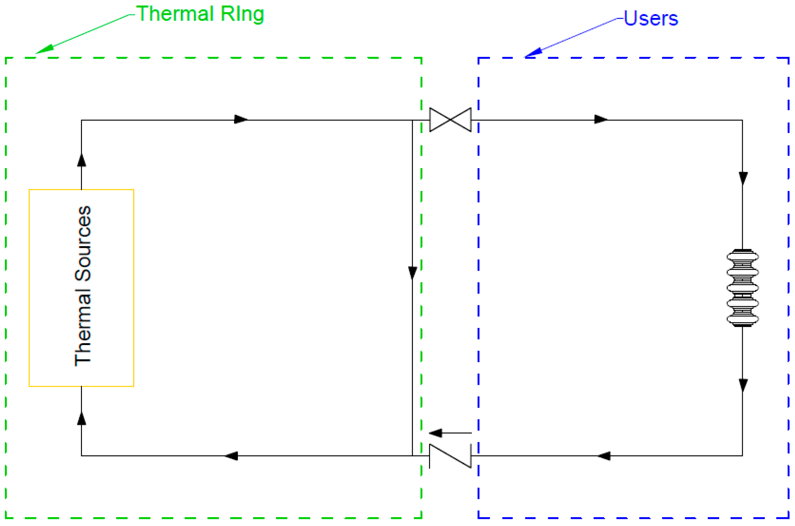
A simple schematic representation of the thermal circuit at the basis of this research work is proposed in Figure 1. In order to meet all these goals, one can consider an equivalent linear electric circuit since it is described by a linear dynamic system; the topology of such a circuit can be derived starting from the well-known parallelism between electric and thermal devices. According to this approach, typically resistors model the thermal losses, capacitors account for thermal inertias and current (voltage) sources represent the power (temperature) generation. In order to meet the first model requirement, the model accounts, as depicted in Figure 1, for a “thermal ring” (TR) and a “user” (U). The first one involves the thermal sources and the thermal network until the buildings, while the second one takes into account the buildings and their interface with the outdoor environment. This latter represents the temperature mean request of an array of homologous end-users (a higher number of rooms) to be considered unique to avoid a significant increase in the system complexity.

The choice of using an equivalent electric representation instead of a purely thermal one is driven by the fact that several EMS for microgrid applications are typically designed to manage the electric part of the grid. For this reason, if an electric equivalent of the system is provided, its integration could be performed in a larger set of EMS tools and would also allow the management of thermal power to be upgraded by retrofitting existing EMS structures.

The proposed equivalent circuit is depicted in Figure 2 and the circuital elements can be described as follows:

• The current source I₀ represents the thermal power generation;
• The capacitance C₀ accounts for the thermal inertia responsible for the time delay necessary to obtain the desired temperature in the heat generator circuit;
• The conductance G₀ models the heat generator circuit losses;
• The voltage source V₀ models the fact that, without any thermal source, the heat generator network temperature approaches the ground temperature;
• The switch $B_1$ models the possible disconnection between the generation and the load (encoded in a Boolean variable S, true when B₁ is open);
• The diode $D_1$ models the fact that the user cannot transfer heat to the water in the heat generator circuit;
• The conductance G₁₁ accounts for the pipe thermal losses in the thermal circuits of the buildings;
• The capacitance C₁ accounts for the thermal inertia responsible for the time delay necessary to obtain the desired temperature at the user side;
• The conductance G₁ represents the thermal losses, which depend on the user insulation;
• The voltage V₁ mimics the fact that, without any thermal source, the user temperature approaches the outdoor ambient one.

In the proposed model, V_C0 is the voltage between terminals A and B and represents the thermal ring temperature, while V_C1, which is the voltage between terminals A₁ and B₁, represents the user mean temperature.

Applying the Kirchoff’s laws to the circuit of Figure 2, one obtains the following set of two ordinary differential equations in the state variables V_C0 and V_C1:

$$\frac{d{V}_{C0}\left(t\right)}{dt}=-\frac{G_0+G_{11}}{C_0}{V}_{C0}\left(t\right)+\frac{G_{11}}{C_0}{V}_{C1}\left(t\right)+\frac{1}{C_0}{I}_0\left(t\right)+\frac{G_{11}}{C_0}{V}_{B1}\left(t\right)+\frac{G_0}{C_0}{V}_0\left(t\right)$$

(1)

$$\frac{d{V}_{C1}\left(t\right)}{dt}=\frac{G_{11}}{C_1}{V}_{C0}\left(t\right)-\frac{G_1+G_{11}}{C_1}{V}_{C1}\left(t\right)-\frac{G_{11}}{C_1}{V}_{B1}\left(t\right)+\frac{G_1}{C_1}{V}_1\left(t\right)$$

(2)

with initial conditions $V_{C0}\left(t_0\right)=V_{C0}^{*}$ and $V_{C1}\left(t_0\right)=V_{C1}^{*}$ at time t₀. Here the voltage V_B1 at the switch B₁ is given by:

$$V_{B1}\left(t\right)=\{\begin{array}{cc}{V}_{C0}\left(t\right)-V_{C1}\left(t\right)& if\mathrm{S}\left(t\right)=\mathrm{true}\\ 0& if\mathrm{S}\left(t\right)=\mathrm{false}\end{array}$$

(3)

The switch is therefore simulated using the Boolean variable S which is equal to one if the switch is open (e.g., during the night period when the TR is disconnected) and is equal to zero if the switch is closed. The numerical solution of (1), (2) allows finding out the time profile of both the TR and U temperatures, given the thermal power generation (which meets the aforementioned requirements of the model).

2.2. Equivalent Electric Circuit Parameters Estimation

Once the topological layout of the network has been defined, it is necessary to define a procedure to evaluate the five parameters proposed by the model: three resistances and two capacitances. One possibility consists of considering the physical layout of the plant and proceeding with a characterization of the elements that compose the system. Nevertheless, such a procedure is computationally complex and affected by uncertainties on the phenomena to be considered. Moreover, the model of the system varies in accordance to the specific thermal network, making difficult to obtain a general procedure to be extended for a generic microgrid asset. To overcome these problems, the methodology adopted in the present paper for parameters estimation relies on an optimization procedure that aims at minimizing the difference between the temperature time profile calculated with (1)–(3) and the measured one. Under this assumption, the only a priori hypothesis is the topology of the circuit, which, by the way, can be judged in an ex-post evaluation comparing the calculated and the measured outputs. The aim of the present section is to present the proposed optimization approach.

As measured temperatures and thermal powers are supposed to be known on a uniform sampling of the interval [t₁, t₂] according to a step Δt and resulting in $N=\left(t_2-t_1\right)/\Delta t+1$ samples, the whole problem will be presented in a discrete form.

As far as the cost function is concerned, the ${\mathsf{\chi }}^2$ function has been chosen, in order to have the possibility of subjecting the obtained trends to a statistical evaluation (i.e., the so called chi-squared test [18] typically used to establish if a theoretical model is incompatible with a set of experimental observations). With specific reference to the available measurements, the cost function for the problem under consideration can be written as:

$${\mathsf{\chi }}_{calc}^2={\displaystyle \sum _{i=1}^N\frac{{(V_{C0}^{meas}(t_i)-V_{C0}(t_i))}^2}{{\mathsf{\sigma }}_{i,\mathrm{C}0}^2}}+\frac{{(V_{C1}^{meas}(t_i)-V_{C1}(t_i))}^2}{{\mathsf{\sigma }}_{i,\mathrm{C}1}^2}$$

(4)

being ${\mathsf{\sigma }}_{i,\mathrm{C}0}$ and ${\mathsf{\sigma }}_{i,\mathrm{C}1}$ the standard deviation of the measured temperature of the thermal ring $V_{C0}^{meas}$ and of the user $V_{C1}^{meas}$, respectively.

The constraints of the problem are the discretized versions of (1) and (2), i.e.,

$$\frac{V_{C0}\left(t_{i+1}\right)}{\Delta t}=V_{C0}\left(t_i\right)\left(\frac{1}{\Delta t}-\frac{G_0+G_{11}}{C_0}\right)V_{C0}\left(t_i\right)+\frac{G_{11}}{C_0}{V}_{C1}\left(t_i\right)+\frac{1}{C_0}{I}_0\left(t_i\right)+\frac{G_{11}}{C_0}{V}_{B1}\left(t_i\right)+\frac{G_0}{C_0}{V}_0\left(t_i\right)$$

(5)

and

$$\frac{V_{C1}\left(t_{i+1}\right)}{\Delta t}=\frac{G_{11}}{C_1}{V}_{C0}\left(t_i\right)+\left(\frac{1}{\Delta t}-\frac{G_1+G_{11}}{C_1}\right)V_{C1}\left(t_i\right)-\frac{G_{11}}{C_1}{V}_{B1}\left(t_i\right)+\frac{G_1}{C_1}{V}_1\left(t_i\right)$$

(6)

The five unknown parameters must belong to reasonable ranges that can be estimated with physical considerations (e.g., the initial estimation of capacitance C₀ can be obtained by the water specific heat multiplied by the overall water mass flowing in the thermal ring).

Moreover, the defined optimization procedure does not require the parameters to be time invariant. As a matter of fact, it seems to be reasonable that they may vary with time in accordance with the specific usage conditions of the rooms (e.g., the number of occupants in a room or the people flowing from one place to another have an impact on the efficiency and inertia of the system). This suggests the possibility of dividing the optimization horizon into time slots, according to the habits of the district fed by the considered thermal network.

Once the optimization problem has been set up, it is necessary to define an algorithm to identify the optimal solution (parameters) to fit the measured data with the proposed model. This is not an easy task, as the cost function (4) that has to be minimized is not a polynomial (the two capacitances appear at the denominator after having inserted (5) and (6) into (4)). To address this problem, a stochastic optimization algorithm has to be preferred in order to avoid possible local minima: the Ant Colony Optimization algorithm (ACO) [19] encodes this characteristic in its nature. In the ACO algorithm, two degrees of freedom are left to the users in order to increase the velocity of convergence and/or emphasize its accuracy. However, to reduce the effect of an inappropriate choice, a different version of the ACO algorithm has here been adopted: the Multivariate Ant Colony Algorithm for Continuous Optimization (MACACO) [20]. MACACO is an extension of ACO based on a covariance matrix instead of a simple variance vector (adopted in ACO).

The updating step for each ant is made such that the new distribution of the solutions points at the promising region is supposedly indicated by the candidate solutions at the previous iteration. This goal can be achieved recalculating this matrix using just 70% of the best solutions found at the present iteration (the 70% value is defined on empirical basis). By doing that, the obtained distribution will go on until the covariance tends to almost zero and is going to be centered at the best optima found.

2.3. Equivalent Electric Circuit Parameters Estimation

The typical thermal network characterization inserted in a microgrid EMS consists of providing the optimization procedure with a constraint stating that the overall thermal power generation must be at least equal to the thermal request (expressed in terms of thermal power) over the optimization time horizon. Unfortunately, this implies to know in advance the time profile of the thermal power request, which is typically predicted by means of the persistency method [21]. This produces a significant amount of uncertainty affecting the overall EMS result.

One of the most interesting applications of the proposed model, for a cogenerative microgrid, is the possibility of integration into an EMS in order to make it able to process the request in terms of temperature profile, which seems much easier to forecast. It is intuitive that for a given load temperature profile, the optimal solution from an economic point of view is given by achieving the minimum amount of primary energy (current in the equivalent modeling) able to guarantee that the room temperature is equal or greater than the desired one.

Recalling the meaning of the electric-thermal equivalency of circuital quantities, it is possible to express the cost function in terms of the I₀ current. In other words, the optimal solution corresponds to the values of I₀(t) that minimize the overall thermal energy in a finite time horizon N_t, i.e.,

$$\min {\displaystyle \sum _{i=1}^{Nt}{I}_0\left(t_i\right)\Delta t}$$

(7)

constrained by (5) and (6) and such that:

$$V_{C1}(t_i)\ge V_{C1}^{des}(t_i)\forall i=1,\dots ,N_t$$

(8)

$V_{C1}^{des}(t_i)$ being the desired value of the load temperature at time t_i.

3. Discussion

3.1. Model Validation in the SPM

This section reports the results obtained by applying the proposed model to the Savona Campus SPM. A complete description of the SPM has been provided in [7,22], but, from a pure thermal point of view, it is worth recalling the SPM’s main features:

• two Combined Heat and Power Gas Turbines (CHP-GT) Capstone C65 model, able to generate 65 kW (electric power) and 112 kW (thermal power);
• one CHP-GT Capstone C30 able to generate 30 kW (electric power) and 55 kW (thermal power);
• two gas boilers characterized by a rated thermal power of 500 kW per boiler.

Figure 3 sketches the SPM map, where a green line groups the TR (composed by the network connections, in red, and the thermal sources, in orange) and the set of blue lines denotes the U (the different buildings). The thermal network is fed by the three cogeneration gas turbines and two gas boilers. The pipes are installed underground and are properly insulated in order to minimize heat losses; the pipe diameters are in the range between DN80 and DN125. Figure 3 does not show the pipes that distribute heat inside each building, where hot water is moved by on/off centrifugal pumps and heat is transferred to the indoor air by means of radiators or fan coils. During winter days, the Campus thermal load can be up to 900 kW of peak request and the thermal energy yearly consumption is about 1300 MWh.

The heating network is monitored in real time by the SPM control room by means of on-field sensors that allow the following variables to be measured: the water mass flow rate, the supply and return lines temperatures, the thermal power output of each gas turbine and boiler and the outdoor temperature. At present, the buildings (U) are not equipped with any sensor measuring the indoor conditions as well as the water temperature and flow rate, so that it is possible to evaluate only the overall thermal load of the Campus but not the single building ones. In the future, each building will be equipped with sensors in order to develop more accurate analyses and to highlight criticalities of the thermal network. However, the rooms’ temperatures have been recorded in the data collection period by means of portable indoor temperature monitoring systems (Elitech RC-4 Mini Temperature Data Logger by Jiangsu Jingchuang Electronics Co. Ltd., Xuzhou, China, 2015 [23]).

As mentioned, in order to attain the goals of the work here presented, a proper set of experimental data had to be collected, on the base of which identifying the model parameters and performing the consistency estimation.

Furthermore, as specified before, the representation of the thermal network has been based on the introduction of an “equivalent” unique end-user U, despite of the large number of actual physical loads. As a consequence, the proper choice of the rooms in which to carry on the temperature measurements had to be identified. In our case, the logic was that of performing the temperature survey within rooms that, even if included in buildings with non-perfectly superimposable thermal characteristics, could be considered as homologous under the temperature requirements of the occupants (offices, apartments, classrooms). In the choice of the rooms to be monitored, particular attention has been devoted in evaluating how the human behaviors (windows opening, room thermostat adjustments, etc.) could affect the thermal profiles within the rooms, trying to minimize these uncontrollable variables.

Operatively, along the survey period the indoor temperature, within the selected rooms, has been acquired continuously and the obtained trends have been recorded weekly. By averaging the data collected in the selected users, a set of day-by-day temperature trends (and the related standard deviations), each of which assumed as representative of the typical user (i.e., room) served by the thermal network, has been obtained.

3.2. Parameter Characterization

The parameters characterization was conducted during the winter season in the period between January 2016 and March 2016. Measurement campaigns were carried out three days per week (Monday and Friday have been avoided because the thermal behavior of the system is influenced in those days by the fact that during weekend the heating system of the whole campus is switched off). The SPM thermal behavior was divided into three different time frames (each one object of parameter identification):

(a)

Time Frame 1: from 10 p.m. to 6 a.m. when the thermal ring stops working and people’s presence inside the buildings is extremely reduced;

(b)

Time Frame 2: from 6 a.m. to 5 p.m. when the building pumping system works and a significant number of people are present inside the buildings;

(c)

Time Frame 3: from 5 p.m. to 10 p.m. when some loads are disconnected from the thermal network and gradually fewer people are present.

As explained before, this suggests considering the circuit parameters as piecewise constant functions throughout the day, i.e.,

$$G_i\left(t\right)=\{\begin{array}{cc}{G}_{i,1}& \mathrm{if}6\mathrm{a}.\mathrm{m}.\le t<5\mathrm{p}.\mathrm{m}.\\ G_{i,2}& \mathrm{if}5\mathrm{p}.\mathrm{m}.\le t<10\mathrm{p}.\mathrm{m}.\\ G_{i,3}& \mathrm{if}10\mathrm{p}.\mathrm{m}.\le t\le 5\mathrm{a}.\mathrm{m}.\end{array}i\in \left\{0,1,2\right\}$$

(9)

$$C_i\left(t\right)=\{\begin{array}{cc}{C}_{i,1}& \mathrm{if}6\mathrm{a}.\mathrm{m}.\le t<5\mathrm{p}.\mathrm{m}.\\ C_{i,2}& \mathrm{if}5\mathrm{p}.\mathrm{m}.\le t<10\mathrm{p}.\mathrm{m}.\\ C_{i,3}& \mathrm{if}10\mathrm{p}.\mathrm{m}.\le t\le 5\mathrm{a}.\mathrm{m}.\end{array}i\in \left\{0,1\right\}$$

(10)

Moreover, condition S(t) becomes true if:

• 0 a.m. ≤ t ≤ 6 a.m. or 10 p.m. ≤ t ≤ 12 p.m., in order to encode condition (a);
• V_C0(t) < V_C1(t), in order to encode the presence of the diode D₁;
• V_C1(t) > V_C1,max(t), where V_C1,max(t) is the user maximum temperature allowed at the instant t.

Once all the measurements were acquired, two thirds of the measurement data were used to train the model (identifying the parameters) while the other third has been used to test the performances of the parameters found. In more detail, data acquired on Tuesday and Thursday of each week were used to choose the optimal values of the parameters, while Wednesday’s data were used for the verification. This choice was made in order to have uniformity in both the identification and validation on the results. The tests have been performed taking the input measurements (ground temperature, environmental temperature and thermal power from the heating ring), calculating the U temperature using the model and then comparing the calculated results with the measured ones.

The optimal values of the circuit parameter (which minimize the cost function) are reported in

Table 1. Optimal Parameters Values.

Parameter	6 a.m.–5 p.m.	5 p.m.–10 p.m.	10 p.m.–6 a.m.
G0 (kW/K)	2.58	3.72	0.40
C0 (kJ/K)	0.93 × 105	2.26 × 105	1.73 × 105
G1 (kW/K)	28.76	24.03	50.01
C1 (kJ/K)	3.91 × 106	3.17 × 106	3.11 × 106
G11 (kW/K)	3.62	20.00	4.01

(all the data used to find the parameter reported in Table 1 are available at Savona Campus and can be provided at request).

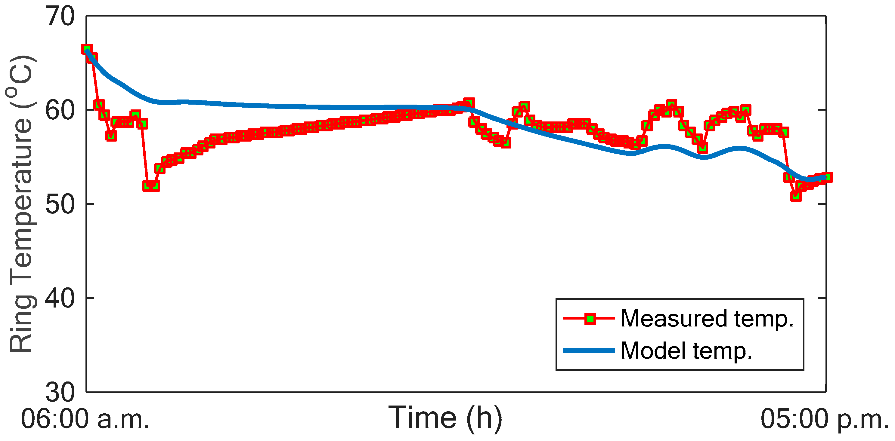
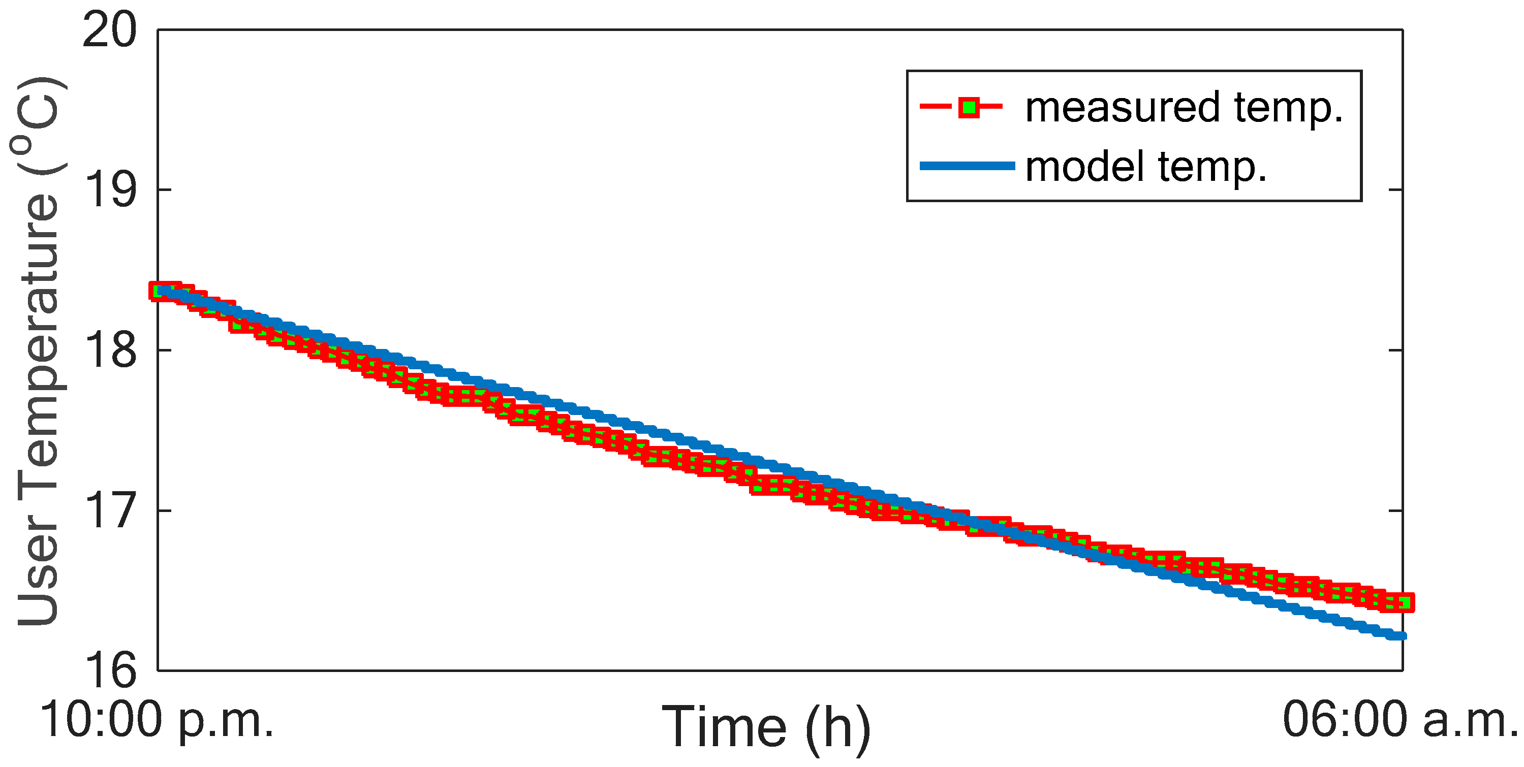
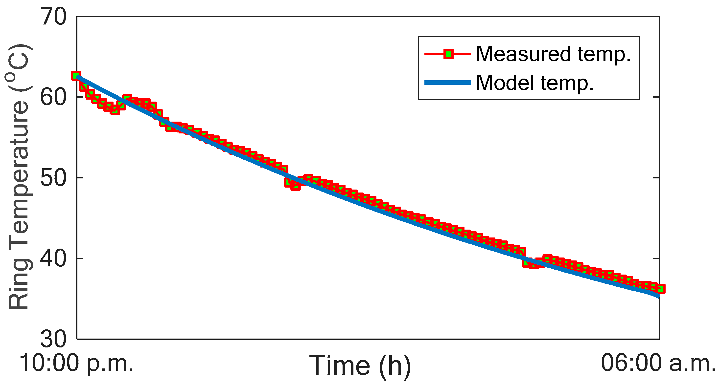
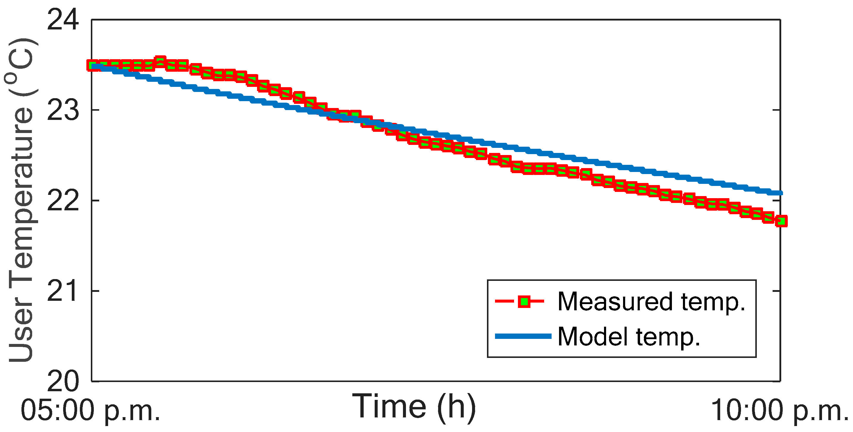
As one can see from Table 1, the results are sensibly different from frame to frame, highlighting the importance of defining a suitable differentiation of the operation assets of the network. Figure 4, Figure 5, Figure 6, Figure 7, Figure 8 and Figure 9 report the results of the tests performed on Wednesday, 20 January 2016. In particular, Figure 4 and Figure 5 plot the user and thermal ring temperature time profiles during nighttime showing an excellent agreement between calculations and measurements. 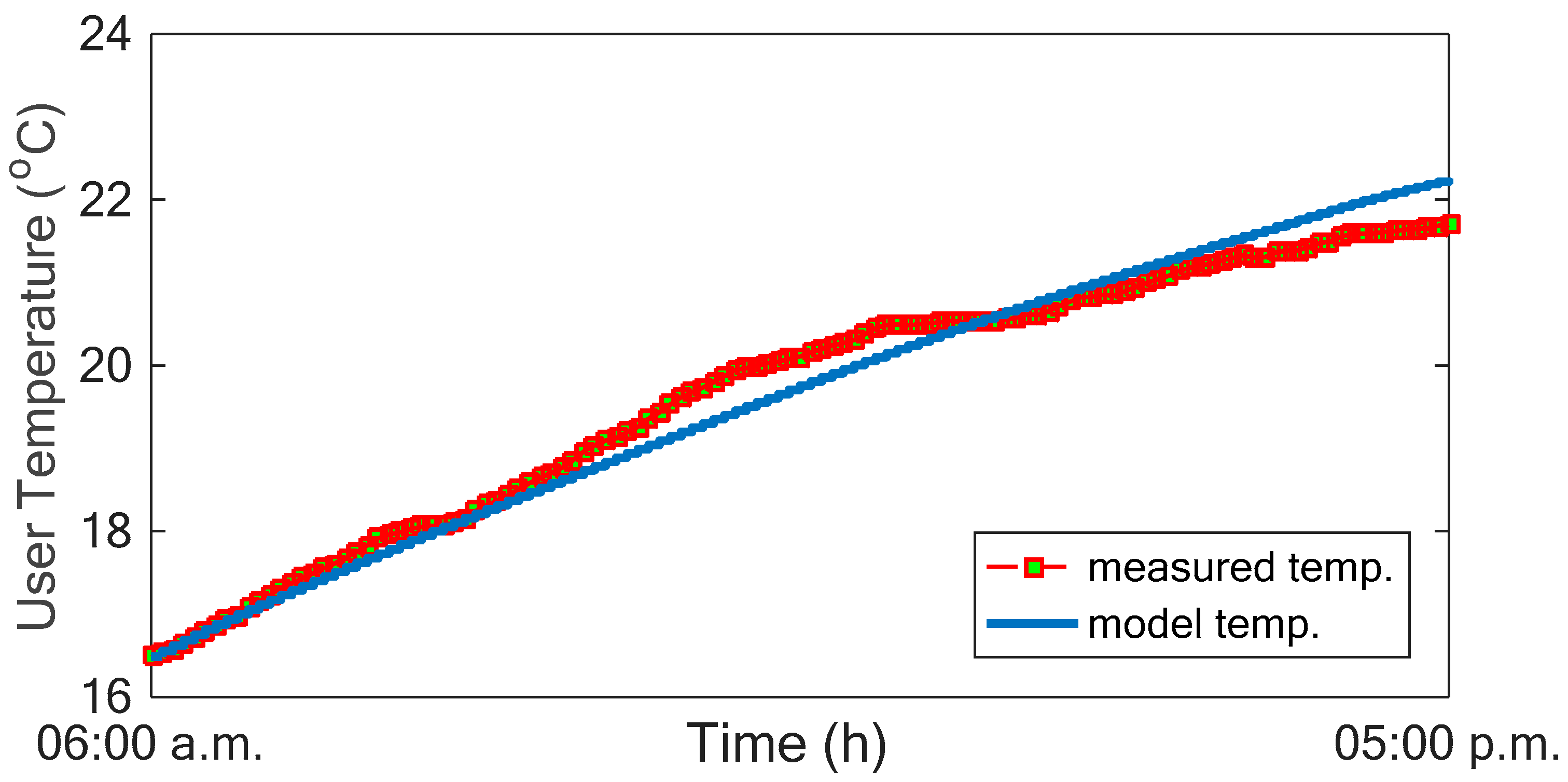Figure 6 and Figure 7 report the comparison of the user and thermal ring temperature during the daytime period, from 6 a.m. to 10 p.m. Once again, the estimated temperature is very close to the measured one with some deviations, especially in the early morning in the graph of the ring temperature. Nevertheless, the maximum error is around 13%, which is anyway a good approximation. It should be observed that for the EMS integration, the most important quantity to be identified is the user temperature, as this is the real user request. 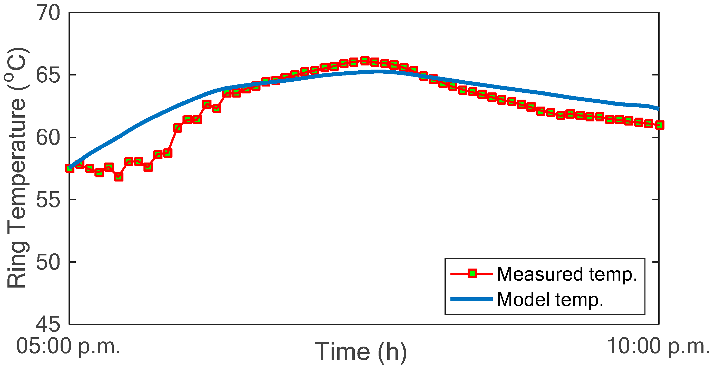Finally, Figure 8 and Figure 9 provide the model validation in the last time frame, from 5 p.m. to 10 p.m. As one can see, the thermal ring temperature is slightly over estimated but the relative error is always lower than 10%.

In order to have an overall evaluation of the accuracy of the proposed model, the value of the chi-squared function has been calculated for the shown testing period and compared to the chi-squared distribution at level α for determining the goodness of fit [15]. To determine the degrees of freedom (d.o.f.) of the chi-squared distribution, it is necessary to consider the total number of acquired measurements (n) and subtracts the number of estimated parameters (in our case 5). The test statistic follows, approximately, a chi-square distribution with (n − 5) degrees of freedom. The more the chi-squared calculated is lower than the chi-squared distribution at level α = 0.95, the more accurate is the result. Moreover, deciding whether a model is in accordance with the data is often summarized by the p-value. According to [24], the more the p-value is close to 1 the more the model is accurate. In

Table 2. Statistics on the testing period.

Timeslot	${\mathsf{\chi }}_{\mathit{c}\mathit{a}\mathit{l}\mathit{c}}^{\mathbf{2}}$	p-Value	${\mathsf{\chi }}^{\mathbf{2}}$ (95%)	dof
6 a.m.–5 p.m.	14.8	~1	39.8	56
5 p.m.–10 p.m.	7.42	~1	92.1	116
10 p.m.–6 a.m.	9.00	~1	68.3	89

the numerical values of all the introduced indicators are reported: the fact that the reference chi-square value is always greater than the calculated one and, in particular, that the p-value extremely close to 1 indicates the high accuracy of the model in describing the thermal phenomena.

3.3. Validation of the EMS Integration

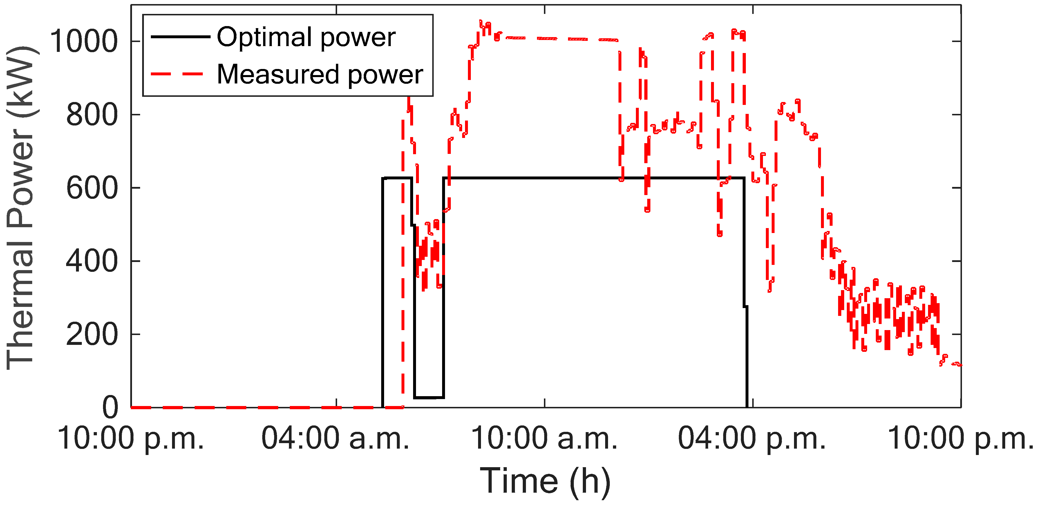
Finally, the proposed model has been implemented in the SPM control system in order to integrate it into the microgrid EMS. The experiment has been performed providing the EMS with the measured temperature and assuming it as the desired temperature; the EMS produced, as output, the thermal power to be provided by the heating units in order to meet the temperature request and minimizing the overall energy over the time horizon. The power request profile is then compared to the real power generation recorded by the SPM Supervisory Control And Data Acquisition (SCADA) system, managed in accordance to the following rules based on the ring temperature T:

• if T < 49 °C, then both boilers switch on
• if 49 °C < T < 53 °C, then only one boiler switches on
• if T > 53 °C, then both boilers switch off

Figure 10 provides the comparison of the thermal power obtained by the EMS (black one) and the actual thermal power profile (red dashed line). As can be noted, the optimal power profile is smother and more constant, providing a saving equal to 1400 kWh along the analyzed 24 h, corresponding to the 12.7% of the total thermal energy requested in the whole day (integrating the thermal power red curve of Figure 10 one obtains 11,050 kWh). From an economical point of view, considering a mean cost of the thermal energy of 0.096 €/kWh (which is the case of the SPM), it is possible to calculate the daily savings as €134 against a total € cost of the non-optimized scenario of €1061. Finally, Figure 11 shows:

i.  

the measured temperature (red dotted line);

ii. 

the temperature calculated feeding the model (1)–(3) with the optimal thermal power profile (black solid line);

iii.

the temperature calculated feeding the model (1)–(3) with the measured thermal power profile (blue dash-dotted line).

This allows us to draw the following conclusions: (a) the comparison between (i) and (ii) shows that the optimal solution is able to reproduce the desired temperature; (b) the good superposition between (i) and (iii) validates once again the effectiveness of the equivalent circuit, as, when fed by the real power, it is able to predict the correct time profile of the temperature; finally, (c) the comparative analysis of (ii) and (iii) states that there can be many different power injections that produce very similar temperature profiles, thus supporting the need to determine the most convenient one.

4. Conclusions

The aim of this contribution has been to propose a simple but general model of a thermal network by means of an equivalent electric circuit. The aim of the present model is to be sufficiently accurate but also simple in order to be integrated into cogenerative microgrid EMSs. The main task of this model is that of linking the thermal power request of the load (usually provided as an input the EMS) to the user temperature (a more meaningful desired parameter for the user). The model proposed is based on a linear equivalent electric circuit whose main parameters can be determined through a measurement campaign applying a parameter identification optimal procedure. The proposed model has been tested in the Savona Campus Smart Polygeneration Microgrid thermal network, in order to show the actual applicability and robustness of the procedure. The values of the parameters involved have been computed by means of an optimization procedure that, in practice, minimizes the difference between the temperature profiles of the thermal circuit and of the user as calculated with the proposed model and the measured ones. The obtained numerical results show that the model describes in a very accurate way the set of measured temperatures and, at the same time, can be easily used as a procedure to optimally schedule the thermal power production leading, to significant thermal energy savings.