Comparison of Cooling System Designs for an Exhaust Heat Recovery System Using an Organic Rankine Cycle on a Heavy Duty Truck

Abstract

A complex simulation model of a heavy duty truck, including an Organic Rankine Cycle (ORC) based waste heat recovery system and a vehicle cooling system, was applied to determine the system fuel economy potential in a typical drive cycle. Measures to increase the system performance were investigated and a comparison between two different cooling system designs was derived. The base design, which was realized on a Mercedes-Benz Actros vehicle revealed a fuel efficiency benefit of 2.6%, while a more complicated design would generate 3.1%. Furthermore, fully transient simulation results were performed and are compared to steady state simulation results. It is shown that steady state simulation can produce comparable results if averaged road data are used as boundary conditions.

1. Introduction

Truck manufacturers develop more efficient propulsion technologies to enable low total cost of ownership to their customers and because of imminent legal CO₂ limits. Current truck engines have a thermal efficiency of up to 46%, and conventional possibilities to further improve this efficiency are limited and costly.

One approach to significantly improve the fuel efficiency is to use an Organic Rankine Cycle (ORC) which can transform a small part of the waste heat produced by the engine into usable mechanical or electrical energy. In 2012, Voith (Zschopau, Germany) used a mechanical system with ethanol as working fluid and a piston expander [1]. In 2015, Lemort [2] presented a mechanical system in a Volvo truck (Gothenburg, Sweden) and an electrical system in an Iveco truck (Arbon, Switzerland). Both were developed in the EU-funded NoWaste project.

The cycle efficiency is influenced strongly by the capability of the cooling system that provides the heat sink for the ORC. In this paper, a detailed, transient and full system simulation model is presented and used to compare different ways to integrate ORC cooling into an existing truck architecture. Espinosa et al. [3] looked at integrating a direct condenser into a French truck and compared different working fluids. The company Cummins (Columbus, IN, USA) used a refrigerant as a working fluid in their exhaust heat recovery (EHR) system in an US truck, which was then cooled in a direct condenser. The cooling system was described in detail; 4% to 5% fuel economy benefits were claimed [4]. Charge air cooler and EHR condenser were placed in parallel in front of the truck cooling system. In a cab-over truck with a limited cooling air mass flow, this approach would lead to high charge air temperatures (intercooler) with a significant increase in fuel consumption.

Using a steam cycle to reduce internal combustion engine fuel consumption is an old idea. Probably, Wilhelm Maybach (Stuttgart, Germany) in 1904 was the first to attempt a realization. It failed because the pressure losses in the exhaust heat exchanger were so high that the overall fuel consumption was higher with steam cycle than without [5].

The use of an ORC system to improve truck fuel efficiency has been subject to research since the 1970s. Back then, Mack Trucks (Greensboro, NC, USA) claimed to have reached a fuel efficiency improvement of more than 10% on a highway test [6]. In 2011, Mack Trucks reduced their fuel efficiency benefit forecast to 2.5 to more than 4% [7].

Hountalas et al. [8] predicted a fuel efficiency improvement of up to 11.3%, based on simulation with working fluid R245ca. A heavy duty truck engine was used as a base, heat sources were charge air (intercooler), exhaust gas recirculation and main exhaust gas. Very optimistic assumptions of boundary conditions regarding all components led to this very high value.

Feru et al. [9] described modeling approach with a focus on the heat exchangers. The system, which has been realized on an engine test bench, seems to be similar to the system regarded in this paper.

Jung [10] described a simple setup which has been realized on the test bench with a Mercedes-Benz EURO V OM457 engine (Stuttgart, Germany). Ethanol has been used as a working fluid and a piston expander as expansion machine. The cycle was open to ambient air, which means a very powerful cooling system had to be used to ensure complete condensation at all times. In addition, a 1.3% fuel efficiency benefit was demonstrated on the test bench and ways to improve it of up to 3.4% are described.

In this paper, the focus is set to the cooling system for an EHR equipped heavy-duty truck, as this has not been reported in literature so far. To simulate the full system, models of all components had to be developed and validated based on engine test bench data and/or vehicle measurement data.

There are numerous ways to design a vehicle cooling system. Here, two different cooling system approaches (floating temperature and low temperature), which have been realized on two different demonstrator trucks at Daimler (Stuttgart, Germany) (Mercedes-Benz Actros and Freightliner SuperTruck) are compared through virtual integration of the low temperature cooling approach into the Actros simulation model. A comparison between different indirect cooling systems can be found by Grelet et al. [11]. This approach to integrating the low temperature cooling cycle into the vehicle is similar to the one chosen here. The high temperature approach, however, is different. On the cooling air side, the vehicle regarded by them is different from the Actros.

The models of both cooling system approaches were stimulated with the same real-live test data, recorded with an Actros production vehicle on a route between Stuttgart and Hamburg, Germany. Both models ran at the same constant ambient temperature of 15 °C.

The Actros engine is an OM471 (Mercedes-Benz, Stuttgart, Germany) with a rated power of 315 kW and a displacement of 12.8 L. The overall weight of the vehicle was 40 t, and it was equipped with a hybrid powertrain that allowed the electrical integration of the expander into the powertrain.

2. Description of the Vehicle Setup

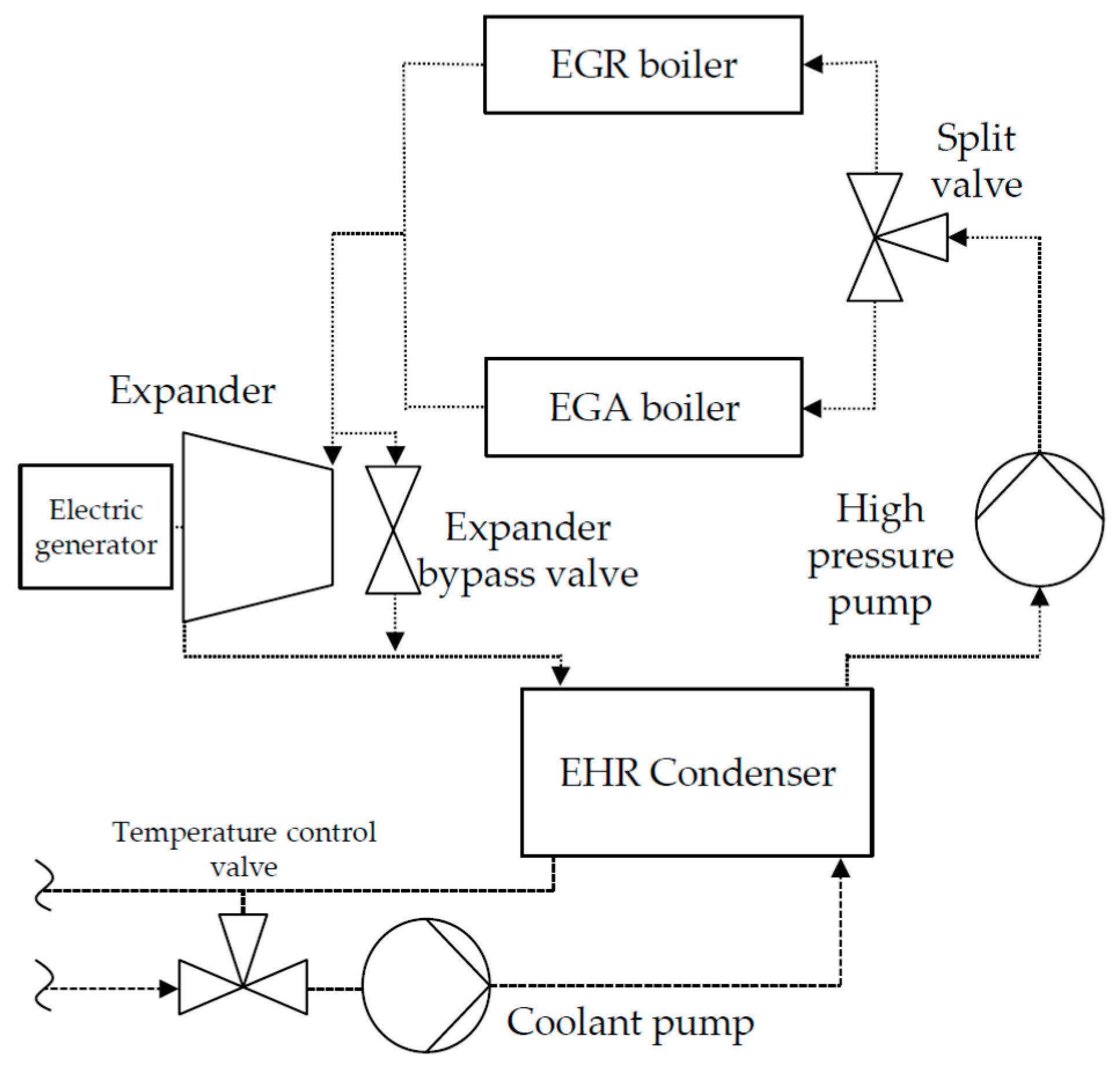
Daimler built an Actros vehicle with an electrically integrated exhaust heat recovery system. The system design is shown in Figure 1. The utilized heat sources were exhaust gas recirculation (EGR) and the tailpipe exhaust downstream the exhaust gas after-treatment system (EGA). As a compromise between simple design and output performance, a parallel setup of both evaporators was chosen. This means, that one high pressure pump, a split valve and one expansion device are sufficient.

The system was designed as a completely hermetic system, similar to AC systems. The working fluid was ethanol, it was chosen as a good compromise between power output, price, safety and environmental friendliness. To design all components, test drive data were used to define five virtual steady state points for the most used engine operating points. Those points differ significantly from steady-state points that were measured on a test bench. The reason is the transient operation that results from real road drive cycles and the high temperature losses between exhaust gas temperature measured downstream, the engine turbocharger, and temperature after EGA.

Table 1. Comparison of road average and steady state test bench boundary conditions, operating point 3. EGA: exhaust gas after-treatment; and EGR: exhaust gas recirculation.

Parameter	Road Average	Test Bench
Engine speed (1/min)	1239	1239
Engine torque (Nm)	1486	1486
EGA temperature (°C)	278.9	390.7
EGR temperature (°C)	460.3	538.8
EGA mass flow (kg/s)	0.242	0.240
EGR mass flow (kg/s)	0.067	0.073

shows an exemplary operating point 3 (1200 min⁻¹, 1500 Nm), and compares steady state engine test bench data to averaged road data.

EGR and EGA mass flows are well comparable between road average data and test bench steady state data. The temperatures, however, are very different. This leads to a significant mismatch if system components are designed for steady state temperatures, and calculations using these temperatures predicting very high, but unrealistic, fuel saving potentials for bottoming cycles.

Figure 2 shows the characteristics of this parallel setup in a T, s-diagram. A typical operating point is displayed featuring the floating temperature cooling system approach. Both evaporators have the same working fluid outlet temperature. The data displayed in Figure 2 can be found in Table 1.

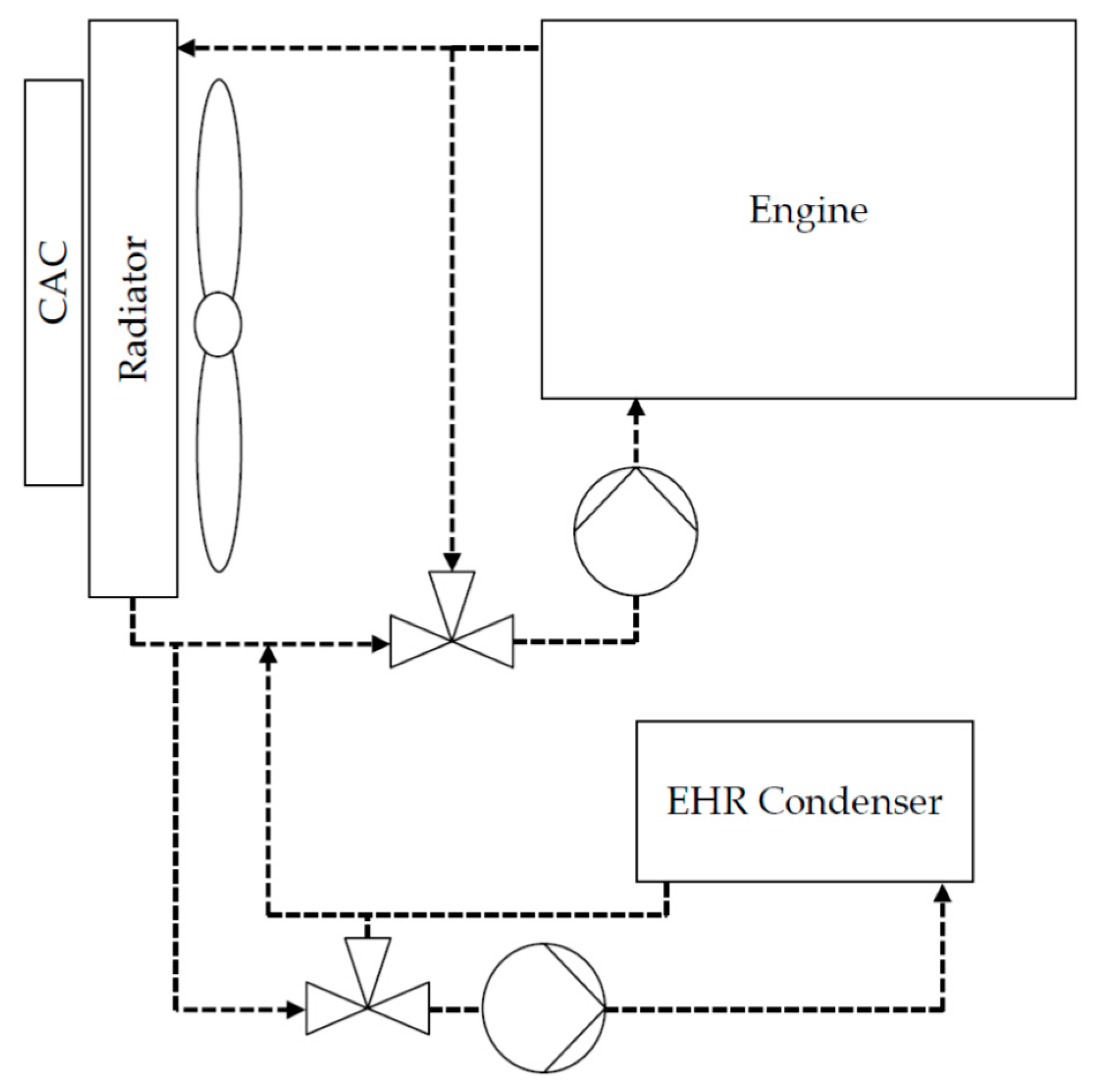
The floating temperature cooling system, which was integrated into the Actros EHR prototype vehicle, is shown in Figure 3. The goal was to integrate an additional water cooled condenser using the existing engine cooling system. To obtain as much power output as possible, the coldest temperature in the cooling cycle was used, that was measured at the outlet of the radiator. This temperature reached up to 103 °C under full cooling system load conditions and very cold temperature (near ambient temperature) at low load. This made an additional temperature control valve necessary, which prevented the temperature from falling below a certain limit. This was necessary to avoid very low condensation pressure that could harm the feed pump (cavitation) and cause unstable working-fluid mass flow.

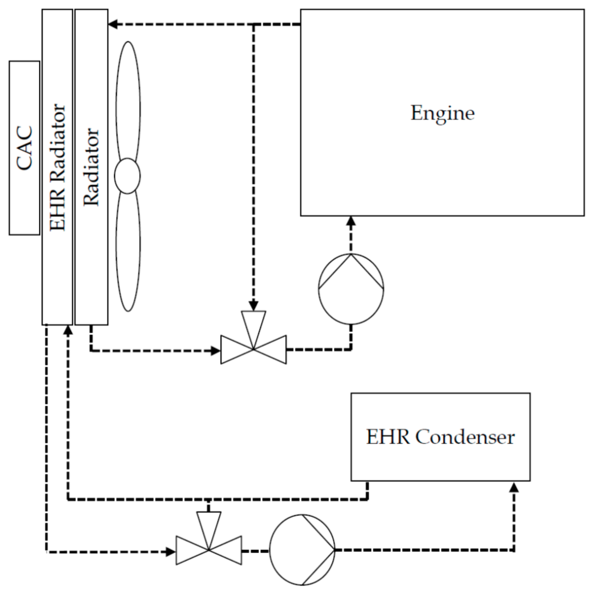
The other approach, similar to the one chosen in the Freightliner Cascadia SuperTruck, was an additional heat exchanger in the front cooling module cooling directly to the ambient air [12]. It is shown in Figure 4. Such a heat exchanger usually can provide a lower coolant temperature compared to the engine cooling cycle. Downstream this additional heat exchanger, the coolant temperature could also be very low; therefore, a temperature control valve was necessary for this approach, too.

Since the bottoming cycle fuel saving potential depends strongly on the heat sink temperature, higher fuel efficiency potential can be expected from the second system. To answer the question how much fuel efficiency can be achieved using each one of the systems, both are integrated into a simulation model and compared.

3. Description of the Simulation Model

The calculation model used in this simulation consisted of two major parts, the vehicle cooling system model and the Rankine evaporator models. Both were setup in GT-Suite [13] as 1-D-models, while the controls and the 0-D expander model were implemented into Matlab Simulink (R2014b, MathWorks, Natick, MA, USA) [14]. Both programs were running in a co-simulation mode. This setup allowed running the detailed GT model with the control software, which is similar to the control software that was used in the vehicle.

3.1. Exhaust Evaporator Model

In the applied model, the exhaust evaporator was simplified to a counter-flow evaporator. The following correlations, included in GT-Suite [15], the Dittus-Boelter correlation for liquid phase and vapor phase heat transfer [16],

$$\mathsf{\alpha }=0.023·R{e}^{0.8}·P{r}^{0.4}·\frac{k}{D},$$

(1)

and the Yan-Lin plate heat exchanger correlation for heat transfer in the two-phase area [15,17],

$$\mathsf{\alpha }=1.926·B{o_1}^{-0.3}·R{e_1}^{0.5}·P{r}^{\frac{1}{3}}·\left(1-x+\sqrt{\raisebox{1ex}{${\mathsf{\rho }}_{liq}$}\!\left/ \!\raisebox{-1ex}{${\mathsf{\rho }}_{vap}$}\right.}\right)·\frac{k}{D},$$

(2)

$$R{e}_1=\frac{G\left(1-x+\sqrt{\raisebox{1ex}{${\mathsf{\rho }}_{liq}$}\!\left/ \!\raisebox{-1ex}{${\mathsf{\rho }}_{vap}$}\right.}\right)D}{{\mathsf{\mu }}_{liq}},$$

(3)

$$B{o}_1=\frac{q^{″}}{G\left(1-x+\sqrt{\raisebox{1ex}{${\mathsf{\rho }}_{liq}$}\!\left/ \!\raisebox{-1ex}{${\mathsf{\rho }}_{vap}$}\right.}\right)·\left(h_{vap}-h_{liq}\right)},$$

(4)

was identified to match the evaporator test bench data.

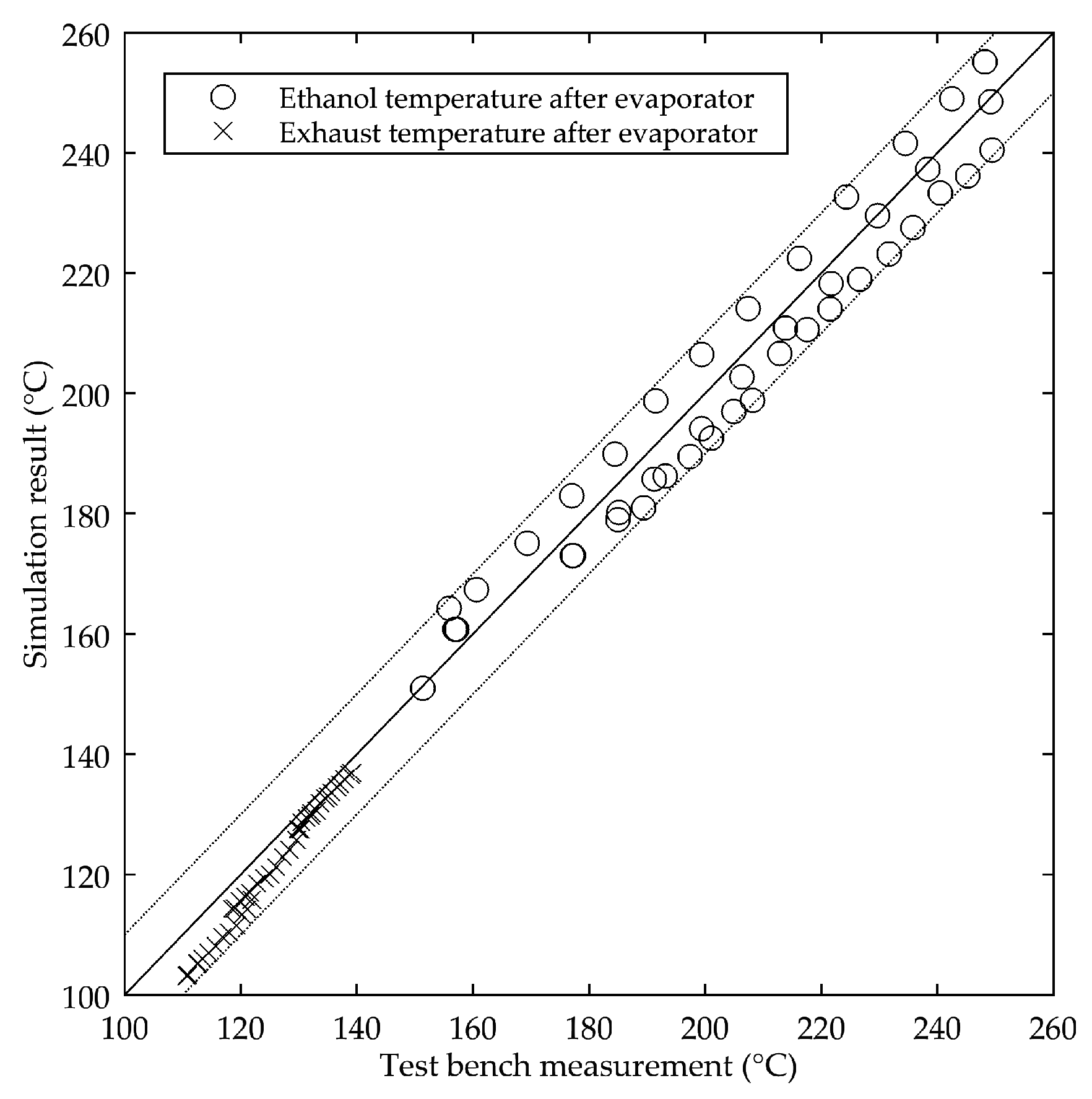
The main influence on heat transfer in the evaporator was not on the working fluid side, but on the exhaust gas side. Therefore, the Nusselt correlation for the exhaust gas side had to be calibrated very carefully. The precision of the heat transfer correlations on the working fluid side is sufficient as shown in Figure 5 and did not have to be modified with heat transfer multipliers. The Nusselt correlation on the exhaust side had the form:

$$Nu=C·R{e}^m·P{r}^{\frac{1}{3}},$$

(5)

$$\mathsf{\alpha }=Nu·\frac{k}{D},$$

(6)

with constants C, m calibrated for laminar, transition and turbulent flow regions.

The accurate pressure loss simulation was found to be very important on both sides of the evaporator. On the exhaust side, high pressure losses caused an increase in fuel consumption due to a rising back-pressure for the engine’s turbine. On the working fluid side, thin channels were used to force an evenly distributed working fluid flow into all plates. These thin pipes caused high pressure losses, especially at high working fluid mass flows. High pressure losses increased the hydraulic power (the working fluid pump has to deliver a higher pressure rise).

The overall evaporator pressure losses were used to calibrate the pressure loss correlation (Müller–Steinhagen–Heck correlation) inside the two-phase region [19]:

$$\frac{dp}{dz}=\left[\frac{dp}{d{z}_{liq}}+2x\left(\frac{dp}{d{z}_{vap}}-\frac{dp}{d{z}_{liq}}\right)\right]{\left(1-x\right)}^{\frac{1}{3}}+\frac{dp}{d{z}_{liq}}{x}^3.$$

(7)

For single phase flow regions, the standard GT-suite correlations were used. Measurement data were fit by using multipliers.

3.2. Exhaust Gas Recirculation Evaporator Model

The EGR evaporator model was set up as a simple counter flow model for calculation time and calculation stability reasons. However, the real evaporator also contained a parallel flow part which improved safety against too high temperatures during sharp transients. The calibration process itself was done the same way as the EGA evaporator. In addition, the same correlations were used to match test bench data.

3.3. Condenser Model

It was not sufficient to calibrate the model for the condenser with test bench data. One important influence on the condenser behavior was the liquid filling level, which could not be measured in the test bench setup. In a hermetic system as used here, the filling level in the condenser is imposed by the high pressure side and the overall system charge. A higher filling level caused less area for condensation and cooling of vapor, which resulted in a higher condensation pressure. The condenser was assumed to be air-free so that the condensation pressure is not increased by the partial pressure of air. Heat transfer model is taken from Yan and Lin [20].

3.4. Expander Model

To represent the impact of the expander on the cycle, a two model approach was chosen. In the cycle model in GT-suite, the expander was represented by a “TurbPosDispRefrig” part. This adiabatic model calculated a volume flow and output power using:

$$\dot{V}=\mathsf{\omega }·\frac{V_i}{{\mathsf{\eta }}_{vol}},$$

(8)

$$P_i=\dot{m}·{\mathsf{\eta }}_i·\Delta h.$$

(9)

The isentropic efficiency and the volumetric efficiency are calculated in a semi-physical model which ran in Matlab Simulink. These two models were sufficient to describe the impact of the expansion machine on the Organic Rankine Cycle by defining the inlet volume flow of the expansion machine, and, therefore, the boiling pressure and the expansion machine outlet enthalpy.

The inner expansion in the volumetric expansion machine was calculated as:

$$P_i=\oint pd\dot{V}=\dot{m}\oint pdV.$$

(10)

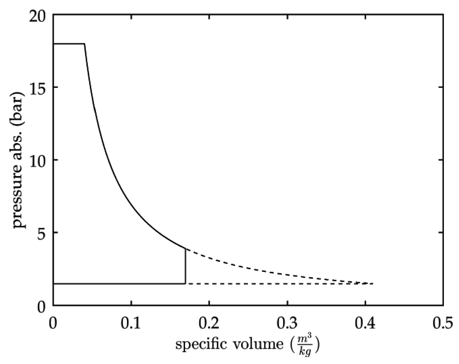
Due to a limited ratio between outlet and inlet volume , the expansion machine showed expansion losses which resulted in a lower . These losses are displayed in Figure 6. Other losses further reduced the system power output. Bearings and seals caused friction, and the electric efficiency had to be considered. These losses did not have direct impact on the rest of the vapor cycle, but on the system power output.

Leakage, however, had a direct impact. Therefore, such effects (higher inlet volume flow and higher expander outlet enthalpy) had to be included into the efficiencies transferred to the GT-Suite turbine part.

To describe leakage and friction properly in every situation, half-empirical correlations based on rotational speed, inlet and outlet pressure were chosen.

3.5. Working Fluid Pump Model

The fluid pump was modeled in a way similar to the expander model. An isentropic efficiency, which included mechanical and electrical losses, was used to calculate the electrical power input. The volume flow and the efficiency were interpolated from lookup tables based on measurement data.

3.6. Split Valve Model

The split valve was modeled by two orifices with varying diameter. The diameter was imposed to represent the overall flow area of each branch of valve outlet.

3.7. Radiator Model

Figure 7 shows the performance map, which was used to fit Nusselt correlation for the radiator on the liquid and the air side. On the x- and y-axis, engine power consumption for engine coolant pumps and fans are shown. The full controllable range is displayed for engine speed 1200 min⁻¹. Slip losses of the viscous clutches were included.

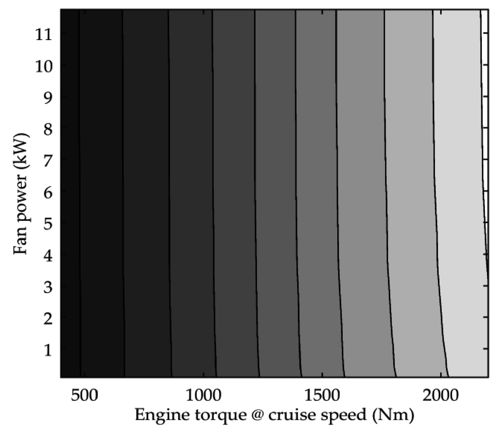
3.8. Charge Air Cooler Model

Figure 8 shows the performance map for the charge air cooler (CAC). Since fan activation obviously had no effect on heat transfer in most situations at cruise speed, the fan was usually not activated because of high CAC outlet temperature. At lower vehicle speed, it could make sense to activate the fan at high engine power because of lower passive cooling ram air mass flow.

3.9. Air Flow through the Radiator Package and Fan Model

A lean approach was chosen to model the air path avoiding excessive calculation time. Figure 9 shows a set of throttle resistances, which were simple orifices with a specified diameter. They were calibrated using steady-state points from wind tunnel measurement data. The inlet throttles represented the resistance of the vehicle front design and the air control system, consisting of a set of flaps in front of the cooling module which, if closed, prevent air flow to improve vehicle aerodynamics. Therefore, the inlet diameters depended on the position of the air control flaps. The backflow resistances represented bypass flow around radiators and fans within the vehicle. At low fan speed and high vehicle speed, air flows through the vehicle might bypass the cooling module. At low vehicle speed and high fan speed, hot air will get in front of the cooling module and corrupt cooling performance. Due to costs and packaging limitation caused by moving parts, it was not possible to seal these back flow areas completely. The outlet throttle represented resistance caused by obstacles in the flow path—like the engine block, auxiliaries and vehicle structure parts. Ram air pressure influence was considered at the flow inlet and outlet. The passive air mass flow through the radiator at cruising speed was about 2.3 kg/s. The increased flow resistance caused by the additional low temperature-radiator reduced this mass flow to about 2.1 kg/s.

3.10. Thermostat Model

The thermostat behavior was crucial for the cooling system behavior, and it was very difficult to predict its behavior precisely. GT-Suite offered an approach which includes time delay and hysteresis, but it was not possible to match the real component behavior satisfactory. Instead, for steady state analysis, a PID (proportional-integral-derivative) controlled valve was used to control the engine inlet temperature. This avoided the hysteresis of the thermostat, and therefore made it easier to compare different setups.

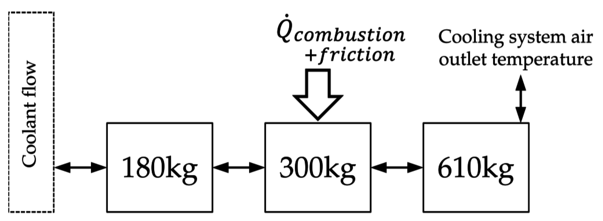
3.11. Thermal Engine Model

The engine block was modelled as a group of connected thermal masses. It was used just to represent the correct transient temperature behavior of the cooling system, since it represents the dominant mass in the system. The heat input into the cooling circuit resulting from the instantaneous engine operating point was interpolated from test bench data. The heat input was calculated using a total enthalpy balance for steady state engine operating points. Three thermal masses, connected to the coolant mass flow and the cooling system air outlet temperature, were used to represent the thermal engine mass. The mass distribution and the heat transfer resistances at the connectors were calibrated to fit transient road data. Figure 10 shows the result of this calibration.

3.12. Solver

The implicit solver in GT-Suite was used for steam cycle calculation, with a time step of 0.2 s. To get a stable solution, especially for very long transient simulations, damping factors and relaxation factors had to be modified. The Simulink control model used a constant time step of 0.1 s to represent the electronic control unit (ECU).

4. Description of the Control Strategy

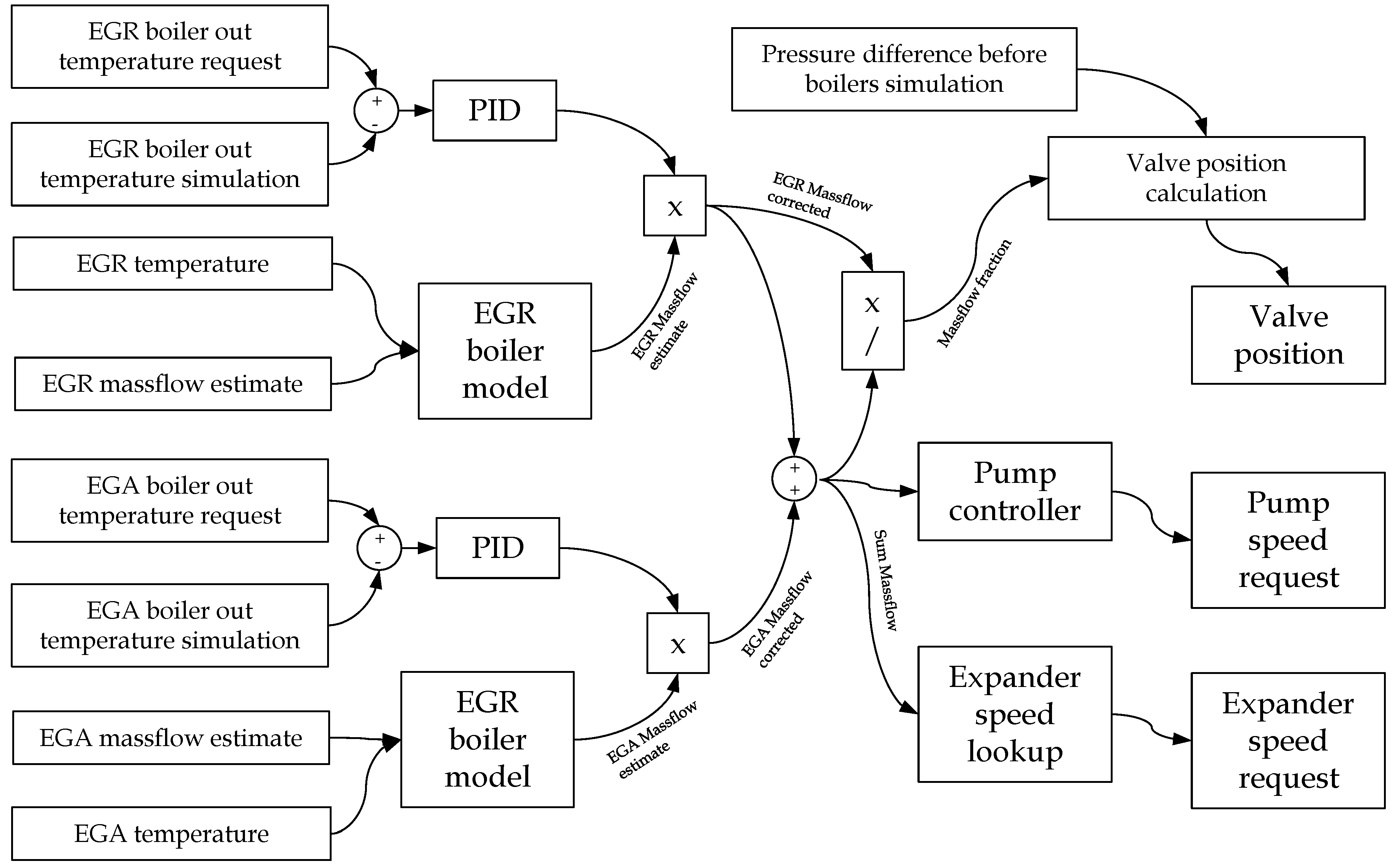
There were several parts in the system which could be controlled individually. The same control strategy was used for steady state and transient simulation. A control flow chart is shown in Figure 11.

4.1. Working Fluid Pump (Rotational Speed)

The Rankine fluid pump had to deliver the overall mass flow to the evaporator s, such that the vapor quality at the expansion machine inlet was always within the given limits. This was a challenging task, especially during sharp transient load changes. The main control was performed by feedforward evaporator models, which estimated a mass flow for each evaporator based on a pinch point approach. This approach was described in detail by Jung [10]. Subsequently, this estimation was then corrected by PID controllers, which were set to keep the evaporator outlet temperature at a desired value. Both corrected mass flows were then added and fed into the pump speed controller, which calculated a pump speed request.

4.2. Working Fluid Split Valve (Position)

The split valve had to distribute the overall mass flow correctly to both evaporators. The position was calculated by solving a pressure difference equation across the valve.

4.3. Expansion Device (Rotational Speed)

In this system, a volumetric expander was used for power generation. The expander speed directly imposed the evaporating pressure for both evaporators. In this simulation, a heat rate based approach to control expander speed was applied. The overall working fluid mass flow was used to calculate the heat input into the system, and based on this information, the expander speed was determined using a look up table. The look up table was filled with expander speeds that ensured maximum system power under certain boundary conditions.

4.4. Exhaust Flap (Position)

The exhaust flap was used to limit the heat input into the system. This could be necessary if the expander generator was at its power limit, or if the cooling system was stressed to an extent that fan and coolant pump would consume more parasitic power than the EHR system could provide. This did happen on hilly roads, especially at high ambient temperatures.

4.5. Expander Bypass Valve (Position)

The expander bypass valve was used to prevent working fluid from entering the expander, when operation is not desired. If the expander path was closed, a bypass was opened to avoid excessive pressure in the system and to keep the cycle running.

4.6. Condenser Coolant Pump (Speed)

The coolant pump control strategy had to make sure that the sub cooling at the working fluid pump inlet was always sufficient. Since the system was hermetically sealed, controlling the coolant volume flow was the only option to ensure sufficient sub cooling. On the other hand, the coolant pump had to make sure that the condensation pressure is lower than the maximum allowable condenser pressure.

Between those boundaries, a condensation pressure and related coolant mass flow could be adjusted to optimize parasitic pump power consumption and EHR system power output.

4.7. Coolant Valve (Position)

The coolant valve was an electrically controlled valve in the prototype vehicle. The control strategy had to make sure that the condenser coolant inlet temperature was always above a defined threshold to keep the condensation pressure near atmospheric pressure. Otherwise, the coolant temperature was controlled to be as cold as possible to maximize EHR power output.

There were two more important components on the engine cooling system which had own control strategies that should not be affected by the EHR system, the vehicle fan and the engine coolant pump.

4.8. Fan and Engine Coolant Pump

The vehicle fan was used to increase the air mass flow through the radiator package. It was often activated at steep grades, when vehicle speed was low and engine load was high for a longer period of time. High engine load implied significant heat input into the cooling system, and at low vehicle speeds, the passive air mass flow through the radiator package was low. Fan activation should be avoided because it caused higher fuel consumption. The engine fan is controlled in a way that sufficient engine cooling was ensured. This was realized by activating the fan slowly if the coolant engine out temperature rose above a certain limit. At low vehicle speeds, the fan might also be activated because of high CAC out temperature.

The engine coolant pump was used to provide sufficient coolant flow to the engine block. The pump speed could be controlled similarly to the controlled fan speed to reduce parasitic power consumption.

To cover transient delays in the fan or pump activation and deactivation, models for the controllable viscous clutches had been integrated.

5. Simulation Results

5.1. Steady State Simulation

To compare both cooling approaches in a proper way, steady-state calculation results using road average data as boundary conditions are shown in

Table 2. Steady state simulation results.

Parameter	Floating Temperature Approach					Low Temperature Approach
Operating point	1	2	3	4	5	1	2	3	4	5
Expander power (kW)	2.79	4.36	5.24	6.50	8.60	2.76	4.40	6.02	8.32	10.7
Condensation pressure abs. (bar)	0.94	1.03	1.90	2.80	3.00	0.93	0.95	0.98	1.01	1.10
Feed pump power (kW)	0.08	0.12	0.18	0.30	0.50	0.08	0.12	0.17	0.29	0.49
Boiling pressure abs. (bar)	11.1	12.5	14.0	16.6	20.1	11.1	12.2	13.0	16.1	19.5
Condenser coolant pump power (kW)	0.02	0.09	0.48	0.48	0.48	0.02	0.04	0.08	0.09	0.46
Fan speed (1/min)	160	160	160	394	683	160	160	160	342	615
Condenser coolant temperature (°C)	60.0	67.0	86.7	97.1	97.1	60.0	60.0	60.0	60.0	65.4
Power gain (%)	3.89	3.18	2.37	2.10	2.41	3.85	3.25	2.99	2.92	3.07
Overall power gain/fuel consumption improvement (%)	2.52					3.09

. The overall power gain was calculated by multiplying the power gain of each point with its work share and adding up the results. The overall benefit of integrating an additional radiator into the vehicle was about 0.6% fuel consumption. The main reason for the better performance of the low-temperature approach was the lower coolant temperature provided to the condenser. In fact, in all operating points except rated power, the temperature had to be lifted artificially by the temperature control valve to protect the working fluid pump from cavitation. It could be concluded that ethanol was not a well-fitting working fluid for such a cooling system. Using an alternative working fluid with lower normal boiling temperature in combination with the low temperature cooling approach would provide appreciable additional fuel consumption reduction potential. Additional measures, like, for example, reducing the main exhaust temperature losses downstream the exhaust gas after-treatment could further improve the system output. Insulating the long exhaust pipe would be an option, or an EGA box placed closer at the engine. This would require unreasonable major changes in the vehicle architecture.

Future fuel consumption improvement measures, like more efficient combustion, better vehicle aerodynamics and low-friction tires will decrease the amount of wasted energy, and also decrease the effect of a waste heat recovery system. Since exhaust temperatures will probably be even lower in future, the benefit from using a separate low temperature cycle for an EHR system will increase compared to a cooling system integrated into the main cooling system.

The impact of coolant temperature on condensing pressure is clearly visible. With the floating temperature system, it climbed up to 3 bar (abs.). This reduced expander power output significantly. Air in the system, which was not possible to avoid completely in the vehicles, increased the condensing pressure to higher values and further decreased system performance. A possibility to remove the air from the system had to be developed, to be able to reproduce the calculated data.

The boiling pressure was similar in both setups. Since the boiling pressure was mainly determined by the expander rotational speed, it was almost independent from the cooling system, except leakage, which increased slightly with lower condensing pressure. Therefore, boiling pressure is slightly higher with the floating temperature cooling system. The heat input into the system is also very similar because of the similar boiling pressure. Working fluid mass flow and also similar working fluid pump power consumption was, therefore, similar.

The coolant pump power consumption, however, was different for both systems. In the case of the low temperature approach, the coolant pump operated at very low power in all points except rated power. Probably, a coolant pump of about half the size would be sufficient for the low temperature cycle. Thus, slight EHR performance penalty for rated power, but lower cost and better efficiency at all other operating points would be achievable.

The fan speed and power consumption were very similar in both cases, but slightly higher compared to a production vehicle.

5.2. Full Transient Simulation

The averaged results from transient simulation are very similar to the steady state simulation results (compare Table 2 and

Table 3. Transient simulation results, averaged.

Parameter	Floating Temperature Approach					Low Temperature Approach
Operating point	1	2	3	4	5	1	2	3	4	5
Expander power (kW)	2.72	4.06	5.41	6.93	8.56	2.96	4.44	5.88	7.82	9.97
Condensation pressure abs. (bar)	1.34	1.47	1.56	1.99	2.86	0.92	0.97	1.03	1.14	1.46
Feed pump power (kW)	0.08	0.13	0.19	0.31	0.51	0.08	0.13	0.19	0.30	0.49
Boiling pressure abs. (bar)	11.6	12.6	13.5	15.9	19.7	11.2	12.2	13.1	15.6	19.2
Condenser coolant pump power (kW)	0.17	0.23	0.25	0.37	0.45	0.05	0.08	0.12	0.21	0.39
Fan speed (1/min)	172	170	170	244	470	171	169	170	234	401
Condenser coolant temperature in (°C)	73.9	77.0	77.5	84.8	95.8	60.4	60.7	61.1	63.6	71.9
Power gain (%)	3.56	2.83	2.57	2.30	2.41	4.09	3.23	2.88	2.68	2.88
Overall power gain/fuel consumption improvement (%)	2.63					3.07

). Some minor differences existed, mainly caused by system and control inertia. The expander power output tended to be higher at low load points and lower at high load points if steady state and transient simulation were compared.

The overall power gain, which was determined using transient simulation results, was very similar to the one which was calculated out of the five virtual steady state points using work share weighting.

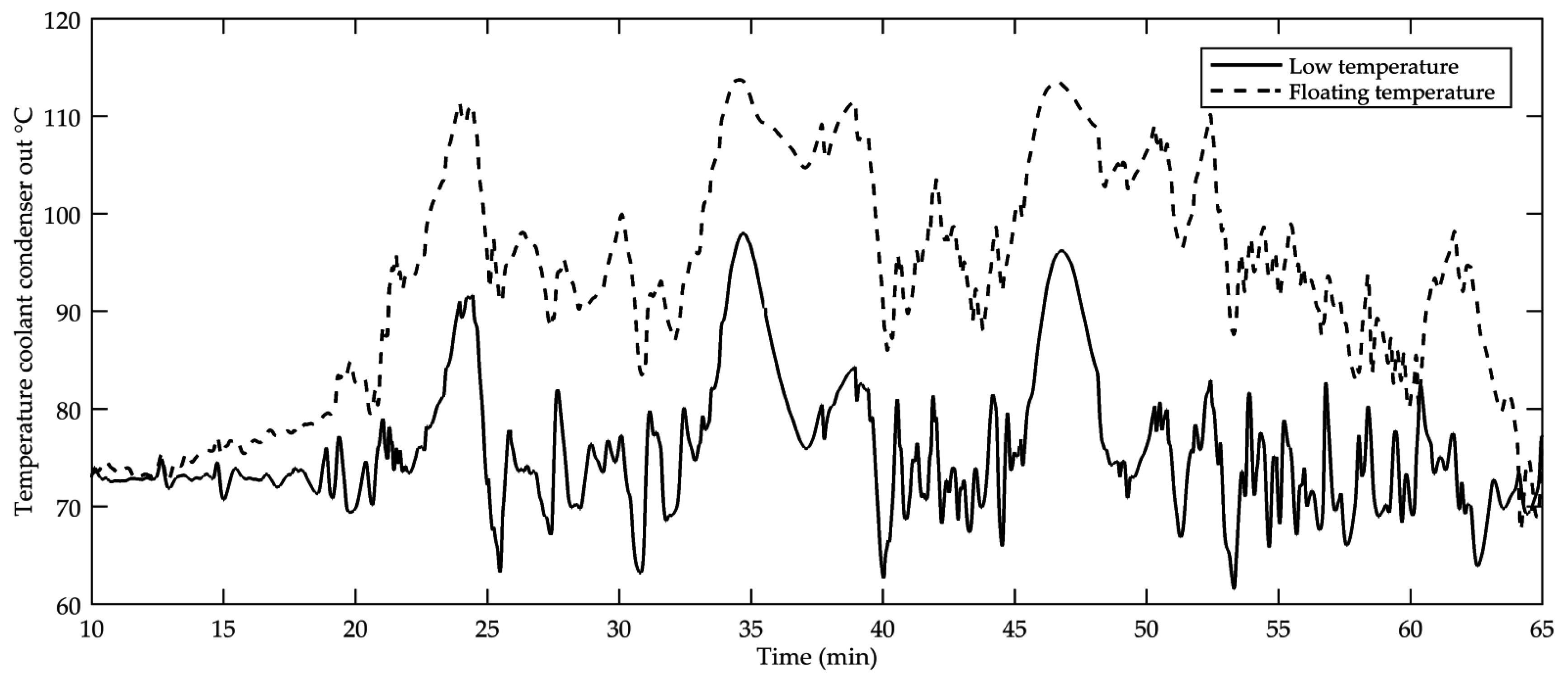
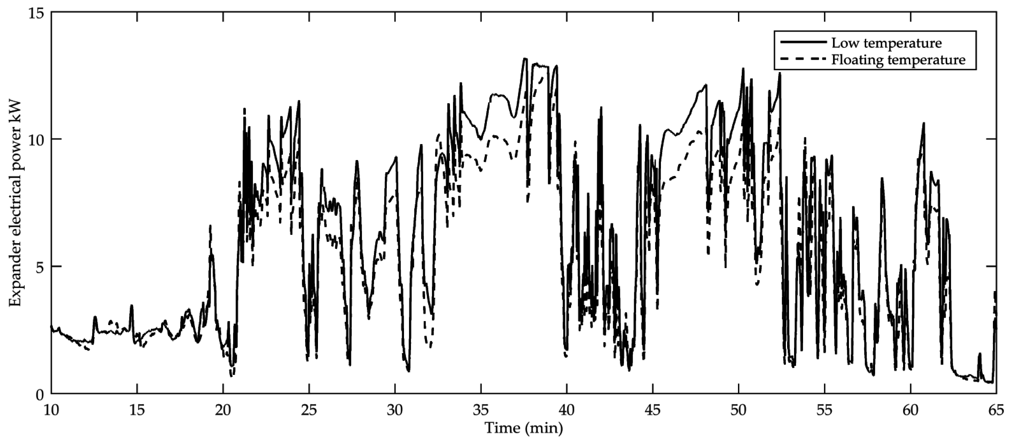
The influence of the cooling system on system performance during transient operation is shown in Figure 12 and Figure 13. The provided track started at Stuttgart, and after about 10 min, the system warm-up was complete and the system started producing power. The warm-up time was shorter than in the measurement since the model is initialized at higher temperatures for better numerical stability. Following the warm-up, three steep grades on the Autobahn from Stuttgart to Munich were found with long engine full load passages.

While the floating temperature system suffered from the high coolant temperatures implied by the engine, the separate cooling system was decoupled from the main one and was able to provide a lower heat removal temperature level to the bottoming cycle. The advantage gained from decoupling of the low-temperature circuit from the main circuit, together with the larger heat transfer area to ambient, exceeded the negative influence of smaller cooling air mass flow through the radiator package.

6. Conclusions

It was possible to create a full transient system model, which was calibrated using data from test bench operation and vehicle tests. The model included the ORC, the vehicle cooling system and simplified controls. The results from transient simulation were similar to those calculated with virtual steady state points. Therefore, it is valid to design an exhaust heat recovery system using virtual steady state points. In this paper, it was shown that the fuel consumption benefit could be increased from 2.63% to 3.07% using an additional full-scale radiator for the EHR system.

Simulation is a useful tool to design an EHR system and its components. It is sufficient to use steady-state points based on average road data, and control strategies can be tested using full transient simulation.

According to Zeitzen [1], a fuel efficiency improvement has to pay itself within two years. Assuming an average fuel consumption of 33 L/100 km, a traveled distance of 100,000 km each year, and a fuel price of €1.2/L, this leads to about €800 for each percent fuel efficiency. This means that the systems considered here may not cost more than €2100 or €2500 to the customer. These figures are small compared to typical installation costs provided by Lemort [2].

Future work will focus on efficiency improvement with working fluids that can make better use of a low temperature cooling system and on measures to reduce the installation cost of an EHR system. With the models described in this paper, sensitivity analyses of hardware modifications and control optimization will be investigated.