Multi-Objective Demand Response Model Considering the Probabilistic Characteristic of Price Elastic Load

Abstract

Demand response (DR) programs provide an effective approach for dealing with the challenge of wind power output fluctuations. Given that uncertain DR, such as price elastic load (PEL), plays an important role, the uncertainty of demand response behavior must be studied. In this paper, a multi-objective stochastic optimization problem of PEL is proposed on the basis of the analysis of the relationship between price elasticity and probabilistic characteristic, which is about stochastic demand models for consumer loads. The analysis aims to improve the capability of accommodating wind output uncertainty. In our approach, the relationship between the amount of demand response and interaction efficiency is developed by actively participating in power grid interaction. The probabilistic representation and uncertainty range of the PEL demand response amount are formulated differently compared with those of previous research. Based on the aforementioned findings, a stochastic optimization model with the combined uncertainties from the wind power output and the demand response scenario is proposed. The proposed model analyzes the demand response behavior of PEL by maximizing the electricity consumption satisfaction and interaction benefit satisfaction of PEL. Finally, a case simulation on the provincial power grid with a 151-bus system verifies the effectiveness and feasibility of the proposed mechanism and models.

1. Introduction

Wind power is one of the fastest growing and cheapest renewable energy sources. In Reference [1], wind power is expected to account for 50% of the world’s clean energy by 2030. However, wind power and other renewable energies are often variable, intermittent, anti-peaking, and difficult to dispatch. In traditional economic dispatch, generation follows the change of load. Therefore, wind power is unsuitable for the operation of a system with a high wind power penetration. The coordinated interactions among power sources, power grid, and loads are studied to address the challenges by optimizing the allocation of resources, such as traditional unit commitment methods and demand response (DR) programs [2,3].

In recent years, many studies [4,5,6,7] have indicated that the uncertainty and forecast errors of wind power have a significant effect on dispatch. Moreover, some studies have recently concluded that a power system can accommodate considerable wind power with high reliability by considering various DR dispatch programs, i.e., DR can be integrated as dispatchable resources that can eliminate wind power output randomness [8,9,10,11]. Reference [12] studied a stochastic unit commitment model for assessing the effects of the large-scale integration of renewable energy sources and deferrable demand in power systems in terms of reserve requirements. In Reference [13], for an electric market with high wind power penetration, a new two-step design approach of forward electricity markets containing DR programs is designed.

In general, DR has the potential to accommodate the uncertainty of wind power output. DR can also benefit consumers [14], ancillary services [15], and even all involved market parties [16]. In this field, deterministic analysis methods for DR behavior have been widely studied [17,18,19]. However, the actual DR is uncertain because of various reasons, including lack of attention, latency in communication, and change in consumption behaviors [20,21,22,23,24]. In the current study, we focus on the uncertainty of the demand response behavior of price elastic load (PEL). In Reference [22], the uncertain region of the price elasticity demand curve varies within a given range. Similarly, the actual price elasticity demand curve is uncertain in nature [23]. This finding indicates that the actual response from consumers in real time can be different from the forecasted values.

The demand response of PEL should be modeled with an uncertain price elasticity demand curve through the preceding analysis. In this paper, a new methodology for analyzing the relationship between the price elasticity and probabilistic characterization of PEL is proposed. Probabilistic characteristics can reflect the uncertainty and subjectivity of demand response behavior under an imprecise price elasticity demand curve. The price elasticity coefficient has a strong leading effect on the error between the real demand response amount and expectation of demand response amount. This study aims to show that the demand curve of PEL can vary within an uncertain range represented by probabilistic mathematical expression. In the aforementioned research, the electricity consumption patterns of end users change via time-varying prices. At the same time, ensuring the satisfaction of electricity customers is an important precondition. Hence, the objective of our optimization model can maximize the electricity consumption satisfaction (ECS) and interaction benefit satisfaction (IBS) of PEL.

The remaining part of this paper is organized as follows. In Section 2, the relationship between the amount of demand response and the efficiency of interactive response is presented. In Section 3, the probabilistic representation and uncertainty range of the PEL demand response are established. In Section 4, both the ECS and IBS of PEL are considered the objectives of stochastic optimization to solve uncertainties from wind power output. A multi-objective optimization method is also developed to solve the problem. In Section 5, a case study is provided and associated simulation results are analyzed. In Section 6, this paper is concluded with a summary of our contributions and conclusions.

2. Stochastic DR Characteristic

This section may be divided by subheadings. It should provide a concise and precise description of the experimental results, their interpretation, as well as the experimental conclusions that can be drawn.

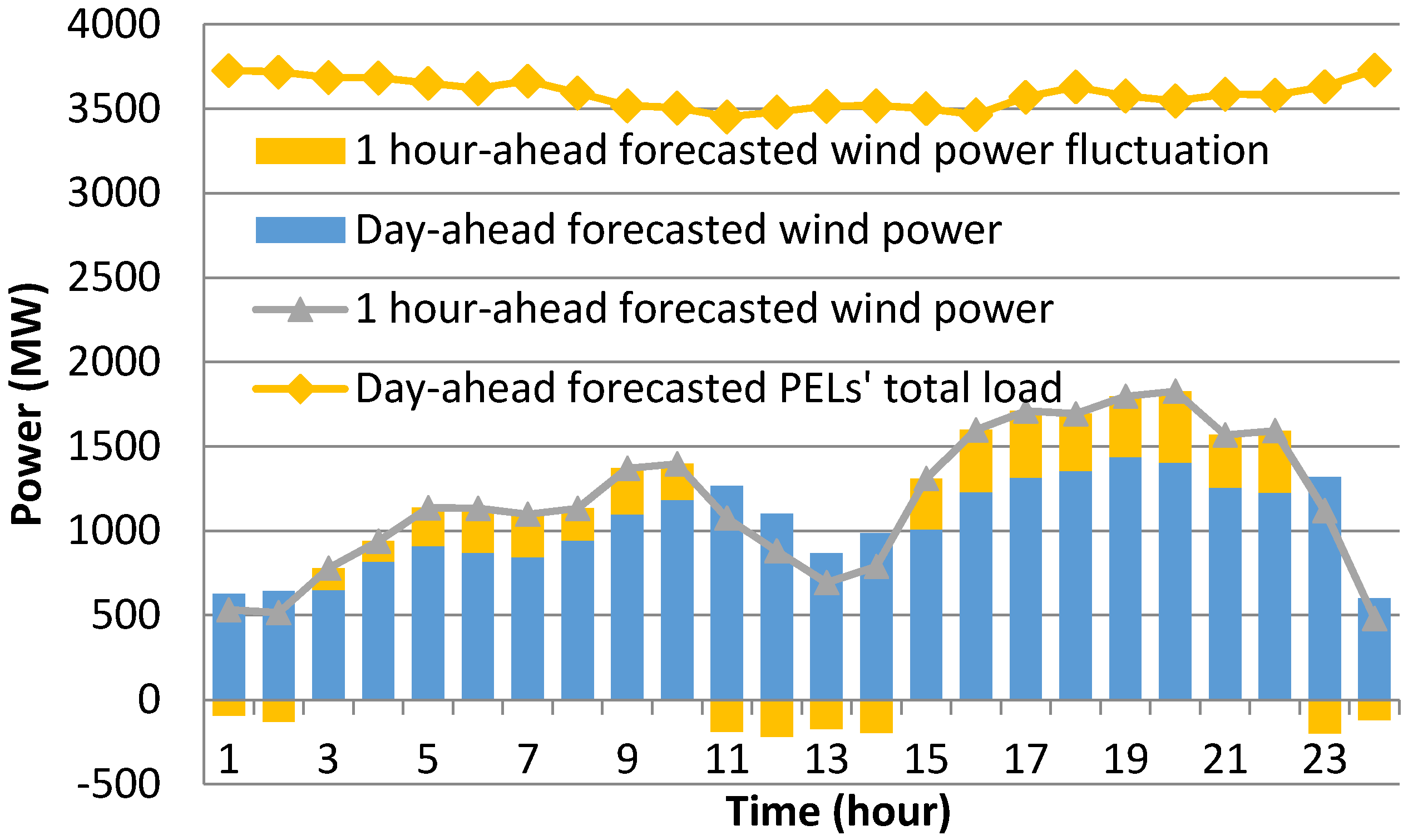
2.1. Demand Response to Balance Wind Power Fluctuations

The anticipated response of PELs can be determined by the static method on the basis of the distributed slack buses [25]. Similarly, we use the static method to determine the allocation of stochastic demand response. Before calculating the probabilistic flow, power imbalance can be allocated to different PELs. Thereafter, the expected demand response amount of each PEL is obtained. Finally, the price signal can be given to each PEL.

The balanced system shows a power imbalance when source-side power fluctuations occur. The imbalance is mitigated by the demand response of PEL. In particular, PEL can increase electricity consumption when wind power is higher than expected. On the contrary, PEL can decrease electricity consumption when wind power output is lower than expected. Finally, the power imbalance of the system can be expressed as follows Equation (1):

$${\displaystyle \sum _{i=1}^N\Delta P_{Gi}}+\Delta P_{Loss}+{\displaystyle \sum _{i=1}^N\Delta P_{l,i}}=0$$

(1)

where, ΔP_Gi and ΔP_l,i are the active power and active load at node i respectively, N is the number of buses, and ΔP_Loss is the change of the transmission loss in the system. The grid change is usually small in a short time. Therefore, $\Delta P_{Loss}$ is negligible. Thus, the interaction benefit of all PELs can be calculated as follows:

$${\displaystyle \sum _{i=1}^N\Delta P_{l,i}}=-{\displaystyle \sum _{i=1}^N\Delta P_{Gi}}$$

(2)

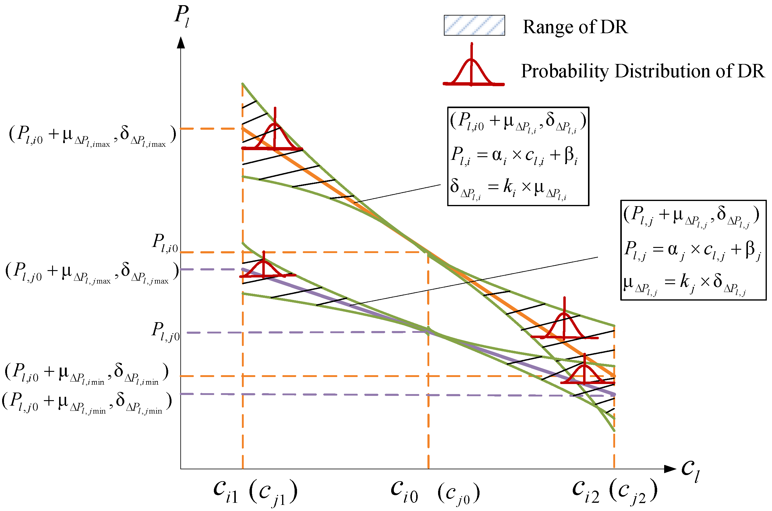
2.2. Probabilistic Characterization of PELs

In the actual demand response process, the price elasticity demand curve is an uncertain issue. We propose a new methodology for analyzing the relationship between the price elasticity and probabilistic characterization of PEL. This methodology emphatically analyzes the effect of different price elasticity coefficients on the error between the real demand response amount and the expectation.

The price elasticity of demand response refers to the sensitivity of demand to price variation [15], which can be expressed as follows:

$$\mathsf{\alpha }=\frac{\partial P}{\partial c}=\frac{c_0}{P_0}\times \frac{dP}{dc}$$

(3)

where, α is price elasticity, which represents the sensitivity of electricity demand (P) with respect to the change of price (c). P₀, c₀ are, respectively, the initial electricity demand and initial price.

The relationship between load i (P_l,i) and its price (c_i) can be defined as follows:

$$P_{l,i}=P(c_i)$$

(4)

We then describe how the explicit formulation of Equation (4) is obtained. According to the PEL defined with price elasticity, a higher price related to the less electricity consumption of PEL. In Reference [15], the relationship between the active power of PEL i (P_l,i) and the price (c_i) is linear and can be expressed as follows:

$$\begin{array}{cc}{P}_{l,i}={\mathsf{\alpha }}_i{c}_i+{\mathsf{\beta }}_i& P_{l,i}\in \left[P_{l,i\min },P_{l,i\max }\right]\end{array},$$

(5)

where, the coefficients α_i < 0 and β_i < 0.

Then, the PEL demand response curves with uncertainties can be described in Figure 1.

Figure 1 illustrates the price elasticity coefficient differs with different PELs. This observation indicates that the degree of PEL sensitivity to price is different. A small value of |α| means low sensitivity to price while a large value of |α| means high sensitivity to price. The price elasticity coefficient of PEL i is smaller than that of PEL j in Figure 1, i.e., |α_i| > |α_j|.

The probability distribution of PEL can be represented in the form of $(P_{i0}+{\mathsf{\mu }}_{\Delta P_i},{\mathsf{\delta }}_{\Delta P_i})$. When the price elasticity coefficient (|α|) is larger, price has a strong leading effect on demand response behavior and the error (${\mathsf{\delta }}_{\Delta P_l}$) between the PEL real demand response amount and expectation is smaller. On the contrary, a smaller price elasticity coefficient means greater uncertainty in demand response behavior because of the greater change in electricity consumption.

Figure 1. Demand response uncertainty curve of PELs.

Figure 1. Demand response uncertainty curve of PELs.

The distribution coefficient of the PEL stochastic parameter is defined as k. The standard deviation and average value meet the following:

$${\mathsf{\delta }}_{\Delta P_l}=k\times {\mathsf{\mu }}_{\Delta P_l}.$$

(6)

On the basis of the preceding analysis, we determine that a smaller price elasticity coefficient (|α|) means a smaller stochastic parameter (k) and that a larger |α| means a larger k; where k_i > k_j. Thus, the uncertain demand response range of PEL i is larger than that of PEL j (Figure 1).

3. PEL Interaction Benefit Model

When PELs participate in grid interactions under the pricing mechanism of electricity markets, their electricity consumption will change with the variation in the relationship of price and power. Thus, electricity expenditure and customer satisfaction are affected.

In general, the relationship between the interaction benefit (C_i) of PEL and its amount of demand response (ΔP_l,i) can be defined as follows:

$$C_i=f\left(\Delta P_{l,i}\right).$$

(7)

The interaction benefit of PEL (C_i) can be defined as the changes in the electricity costs of customers.

$$C_i=P_{l,i0}\times c_{i0}-P_{l,i}\times c_i.$$

(8)

Equation (5) can be transformed into Equation (9):

$$c_i=\frac{1}{{\mathsf{\alpha }}_i}{P}_{l,i}-\frac{{\mathsf{\beta }}_i}{{\mathsf{\alpha }}_i}.$$

(9)

We can obtain Equation (10) by substituting Equation (9) into Equation (8):

$$C_i=-\frac{1}{{\mathsf{\alpha }}_i}\times {P_{l,i}}^2+\frac{{\mathsf{\beta }}_i}{{\mathsf{\alpha }}_i}\times P_{l,i}+P_{l,i0}\times c_{i0}.$$

(10)

In this paper, the relationship between P_l,i and ΔP_l,i can be expressed as follows:

$$P_{l,i}=P_{l,i0}+\Delta P_{l,i}.$$

(11)

The relationship between C_i and ΔP_l,i can be described as Equation (12) by substituting Equation (11) into Equation (10):

$$C_i=-\frac{1}{{\mathsf{\alpha }}_i}\times \Delta {P_{l,i}}^2+\frac{{\mathsf{\beta }}_i-2P_{l,i0}}{{\mathsf{\alpha }}_i}\times \Delta P_{l,i}.$$

(12)

4. Stochastic DR Model of PEL

4.1. Demand Response Satisfaction of PEL

The demand response satisfaction of PEL is considered the optimization objective in the demand side. Demand response satisfaction can be measured in two ways: one is electricity consumption satisfaction (ECS), and the other is interaction benefit satisfaction (IBS). In this paper, we define the ECS of PEL and the IBS of PEL as the index to measure the variation of electricity consumption manner and the index to measure the variation of customer electricity costs, respectively.

Before demand response occurs, the electricity consumption manner of PEL should be arranged. At this time, ECS reaches the maximum point. After demand response occurs, PEL changes the electricity consumption manner to pursue the maximum demand response interaction benefit. Thereafter, the PEL comfort of electricity consumption is changed.

The ECS of PEL is established in the response of load and its original level:

$${\mathsf{\eta }}_i=1-\left|\Delta P_{l,i}\right|/P_{l,i},$$

(13)

where η_i represents the ECS of PEL i, and ECS submits to ${\mathsf{\eta }}_i\in (0,1]$. ECS reaches the maximum (its value is 1.0) when the electricity consumption manner of PEL is not changed.

Combined with the model of the load response interaction benefit described in Section 2, the IBS of PEL is expressed as follows:

$$\begin{array}{l}{\mathsf{\epsilon }}_i=1+\frac{P_{l,i0}\times c_{i,0}-P_{l,i}\times c_i}{P_{l,i0}\times c_{i,0}}\\ =1+\frac{-\frac{1}{{\mathsf{\alpha }}_i}\times \Delta {P_{l,i}}^2+\frac{{\mathsf{\beta }}_i-2P_{l,i0}}{{\alpha }_i}\times \Delta P_{l,i}}{P_{l,i0}\times c_{i,0}}\end{array}.$$

(14)

4.2. Probabilistic Demand Response Model

4.2.1. Objective Function

The maximum demand response satisfaction of PEL is considered to be the objective in the load side. Thereafter, by considering the probabilistic demand response of PEL, we maximize the expected demand response satisfaction of various PELs:

$$\{\begin{array}{l}\begin{array}{cc}\max & E\left({\mathsf{\eta }}_1^t\right),\cdots ,E\left({\mathsf{\eta }}_i^t\right),\cdots ,E\left({\mathsf{\eta }}_{N_{PL}}^t\right)\end{array}\\ \begin{array}{cc}\max & E\left({\mathsf{\epsilon }}_1^t\right),\cdots ,E\left({\mathsf{\epsilon }}_i^t\right),\cdots ,E\left({\mathsf{\epsilon }}_{N_{PL}}^t\right)\end{array}\end{array},\forall t=1,2,\cdots 24,$$

(15)

where, $E(\ast )$ represents the mathematical operator of expectation at time t hour.

The objective function is a multi-objective optimization problem. The objective function weighting is introduced to transform the problem into a single-objective optimization problem. Thus, the demand response satisfaction of PEL should be the weighted average number of ECS and IBS. Thereafter, the demand response satisfaction of PEL i is transformed as follows:

$$\max \begin{array}{c}\end{array}E\left(f_i^t\right)=E\left({\mathsf{\lambda }}_{i1}{\mathsf{\eta }}_i^t+{\mathsf{\lambda }}_{i2}{\mathsf{\epsilon }}_i^t\right),$$

(16)

$${\mathsf{\lambda }}_{i1}+{\mathsf{\lambda }}_{i2}=1,$$

(17)

where, λ_i1 represents the weight of IBS and λ_i2 represents the weight of ECS. With regard to different PELs, weights can be set as different values to reflect that the degrees of attention to IBS and ECS are different for various PELs.

The following can be obtained by substituting Equations (13) and (14) into Equation (18):

$$\begin{array}{l}E\left(f_i^t\right)=E\left(\begin{array}{l}{\mathsf{\lambda }}_{i,1}\times \left(1-\frac{\Delta P_{l,i}^t}{P_{l,i0}^t}\right)\\ +{\mathsf{\lambda }}_{i,2}\times \left(1+\frac{-\frac{1}{{\mathsf{\alpha }}_i}\times \Delta {P_{l,i}^t}^2+\frac{{\mathsf{\beta }}_i-2P_{l,i0}}{{\mathsf{\alpha }}_i}\times \Delta P_{l,i}^t}{P_{l,i0}^t\times c_{i,0}^t}\right)\end{array}\right)\\ ={\mathsf{\lambda }}_{i,1}\times \left(1-\frac{E\left(\Delta P_{l,i}^t\right)}{P_{l,i0}^t}\right)\\ +{\mathsf{\lambda }}_{i,2}\times \left(1+\frac{-E\left(\Delta {P_{l,i}^t}^2\right)+\left({\mathsf{\beta }}_i-2P_{l,i0}^t\right)\times E\left(\Delta P_{l,i}^t\right)}{{\mathsf{\alpha }}_i\times P_{l,i0}^t\times c_{i,0}^t}\right)\end{array}.$$

(18)

The objective function includes $E(\Delta {P_{l,i}^t}^2)$ and $E(\Delta P_{l,i}^t)$, which are expressed as follows:

$$E\left(\Delta {P_{l,i}^t}^2\right)={\displaystyle {\int }_{-\infty }^{+\infty }(\Delta {P_{l,i}^t}^2\times f(\Delta P_{l,i}^t))d\Delta P_{l,i}^t},$$

(19)

$$E(\Delta P_{l,i}^t)={\displaystyle {\int }_{-\infty }^{+\infty }(\Delta P_{l,i}^t\times f(\Delta P_{l,i}^t))d\Delta P_{l,i}^t},$$

(20)

According to probability theory, if $\left[\begin{array}{cc}a,& b\end{array}\right]$ is the range of $\Delta P_{l,i}^t$, then $\Delta P_{l,i}^t$ follows a normal distribution $N({\mathsf{\mu }}_{\Delta P_{l,i}^t},{\mathsf{\delta }}_{\Delta P_{l,i}^t}^2)$. If $\Delta P_{l,i}^t$ submits to $\left[\begin{array}{cc}\mathsf{\mu }-3\mathsf{\delta },& \mathsf{\mu }+3\mathsf{\delta }\end{array}\right]\in \left[\begin{array}{cc}a,& b\end{array}\right]$, the confidence is 99.7% and can be approximated to one. Thereafter, we convert Equations (19) and (20) to Equations (21) and (22), respectively:

$$E(\Delta {P_{l,i}^t}^2)={\mathsf{\mu }}_{\Delta P_{l,i}^t}^2+{\mathsf{\delta }}_{\Delta P_{l,i}^t}^2,$$

(21)

$$E(\Delta P_{l,i}^t)={\mathsf{\mu }}_{\Delta P_{l,i}^t}.$$

(22)

4.2.2. Equality Constraints

According to the description in Section 3, the demand response of PEL should meet the following two conditions:

• Power balance constraints

When wind power fluctuation causes system power imbalance, the fluctuations are absolutely eliminated by the demand response of PEL:

$$\Delta P_{\sum L}^t={\displaystyle \sum _{i=1}^{N_{PL}}E(\Delta P_{l,i}^t)},$$

(23)

where $\Delta P_{\sum L}^t$ is the power imbalance caused by wind power output fluctuations at time t hour.

• Stochastic Constraint

The actual demand response is uncertain. The relationship between standard deviation (${\mathsf{\delta }}_{\Delta P_{l,i}^t}$) and the average value (${\mathsf{\mu }}_{\Delta P_{l,i}^t}$) of PEL i is expressed as follows:

$${\mathsf{\delta }}_{\Delta P_{l,i}^t}=k_i\times {\mathsf{\mu }}_{\Delta P_{l,i}^t}.$$

(24)

The distribution coefficient of the PEL i stochastic parameter $k_i$ is strongly affected by the price elasticity coefficient ($\left|{\mathsf{\alpha }}_i\right|$).

4.2.3. Inequality Constraints

When load increases, demand response constraints are expressed as follows:

$$\begin{array}{l}\Delta {P_{l,i}^t}^{-}\ge 0\\ \Delta {P_{l,i}^t}^{+}\le P_{l,i\max }^t-P_{l,i0}^t\end{array}.$$

(25)

When load decreases, the demand response constraints are expressed as follows Equation (26):

$$\begin{array}{l}\Delta {P_{l,i}^t}^{-}\ge P_{l,i\min }^t-P_{l,i0}^t\\ \Delta {P_{l,i}^t}^{+}\le 0\end{array},$$

(26)

where $(\Delta {P_{l,i}^t}^{-},\Delta {P_{l,i}^t}^{+})$ is PEL response random fluctuation range.

4.3. Solution Methodology

We introduce the weight of the objective function to solve the multi-objective optimization problem, and Equation (16) can be transformed to Equation (27):

$$\begin{array}{cc}\max & {\displaystyle \sum _i^{N_{rl}}{\nu }_i\times E\left(f_i^t\right)}\end{array}.$$

(27)

Finally, the objective function switches to a non-linear optimization problem. We use the particle swarm optimization (PSO) [26] to solve this model.

5. Case Study

5.1. Data and Assumptions

The provincial power grid, which is a main network with 220 kV and 330 kV in Northwest China, contains 151 buses, 252 lines, and 43 generators. The total installed capacity is 24 GW. 11 buses are wind-driven generator with 4 GW capacity. The day-ahead forecasted wind output power and the total load of PEL are predicted in Figure 2. Moreover, a one-hour-ahead forecasted wind power is assumed to have deviation (Figure 2).

Figure 2 illustrates that the one-hour-ahead forecasted wind power fluctuates by the day-ahead forecasted wind output power. When the real-time wind power output is at the day-ahead power value, the power of system is in balance. The power imbalance can be calculated when the wind power output fluctuates. If the value is positive, a power surplus occurs. Moreover, a negative value shows a lack of generator power. Decreasing the load power consumption is needed in this situation.

Assuming that, there will be sufficient PEL to balance the variation in wind. Eight load buses are selected as PELs. The parameters of the price response curve and the weight values of the demand response satisfaction of PELs are presented in Table 1.

Figure 2. Forecasted Wind Power and PEL Load.

Figure 2. Forecasted Wind Power and PEL Load.

Table 1. Weight Values of PEL Response Satisfaction.

PEL	αi	βi	λi1	λi2
1	−0.559	9.3403	0.7	0.3
2	−0.509	8.3973	0.7	0.3
3	−0.506	5.3461	0.6	0.4
4	−0.556	4.1522	0.6	0.4
5	−0.107	3.2877	0.5	0.5
6	−0.117	3.2574	0.5	0.5
7	−0.306	2.9123	0.4	0.6
8	−0.336	2.9642	0.4	0.6

Table 1. Weight Values of PEL Response Satisfaction.

PEL	αi	βi	λi1	λi2
1	−0.559	9.3403	0.7	0.3
2	−0.509	8.3973	0.7	0.3
3	−0.506	5.3461	0.6	0.4
4	−0.556	4.1522	0.6	0.4
5	−0.107	3.2877	0.5	0.5
6	−0.117	3.2574	0.5	0.5
7	−0.306	2.9123	0.4	0.6
8	−0.336	2.9642	0.4	0.6

The price elasticity coefficient α_i and β_i of each PEL bus can be calculated as Table 1. We then set the corresponding distribution coefficient of probabilistic parameter k_i.

We can also know that the price elasticity coefficients satisfy $\left|{\mathsf{\alpha }}_4\right|>\left|{\mathsf{\alpha }}_1\right|>\left|{\mathsf{\alpha }}_3\right|>\left|{\mathsf{\alpha }}_2\right|$$>\left|{\mathsf{\alpha }}_8\right|>\left|{\mathsf{\alpha }}_7\right|>\left|{\mathsf{\alpha }}_6\right|>\left|{\mathsf{\alpha }}_5\right|$, thus indicating that the sensitivity to price of PEL 5 is the smallest and that of PEL 4 is the largest. On the basis of the analysis in Section 2.2, a smaller price elasticity coefficient $\left|\mathsf{\alpha }\right|$ leads to a stronger response leading role, and a smaller response deviation than expected. Thus, k_i decreases. On the contrary, a larger $\left|\mathsf{\alpha }\right|$ corresponds to the greater uncertainty of demand response. Thus, k_i increases. Therefore, $k_4>k_1>k_3>k_2>k_8>k_7>k_6>k_5$. In this paper, the following are set: $k_4=0.25$, $k_1=0.2$, $k_3=0.18$, $k_2=0.15$, $k_8=0.12$, $k_7=0.1$, $k_6=0.08$, and $k_5=0.05$.

The day-ahead forecasted PEL nodal prices are assumed, as shown in Figure 3.

Figure 3. Day-ahead forecasted PEL nodal prices.

Figure 3. Day-ahead forecasted PEL nodal prices.

5.2. Relationship between Wind Power Fluctuation and Demand Response Amount

By using the simulation that considers the parameters shown in Figure 2 and Figure 3, and Table 1, the calculation results of PEL demand response amounts are shown in Figure 4, the one-hour-ahead nodal prices are shown in the Figure 5, and demand response satisfactions are shown in Figure 6 and Figure 7.

Figure 4. Demand response amounts of PEL.

Figure 4. Demand response amounts of PEL.

Figure 5. One-hour-ahead PEL nodal prices.

Figure 5. One-hour-ahead PEL nodal prices.

Figure 6. Electricity consumption satisfaction (ECS) of PELs.

Figure 6. Electricity consumption satisfaction (ECS) of PELs.

Figure 7. Interaction benefit satisfaction (IBS) of PELs.

Figure 7. Interaction benefit satisfaction (IBS) of PELs.

Figure 4 illustrates that PELs show the overall responses to wind fluctuation. The comparison of Figure 3 and Figure 5 indicates that each one-hour-ahead PEL nodal price at time 11:00–15:00 is higher than the day-ahead nodal price. Furthermore, each PEL decreases the load power consumption because the wind fluctuation is negative and the generator power is lacking. Figure 6 and Figure 7 show the demand response satisfaction of PEL. A higher demand response at PEL 1–4 leads to a smaller ECS is, but the greater IBS and demand response overall satisfaction are. The reason is that IBS factor and ECS factor of PEL 1, 2 and PEL 3, 4 are (0.7, 0.3) and (0.6, 0.4), respectively. In particular, the factor of IBS is equal or greater than the factor of ECS factor.

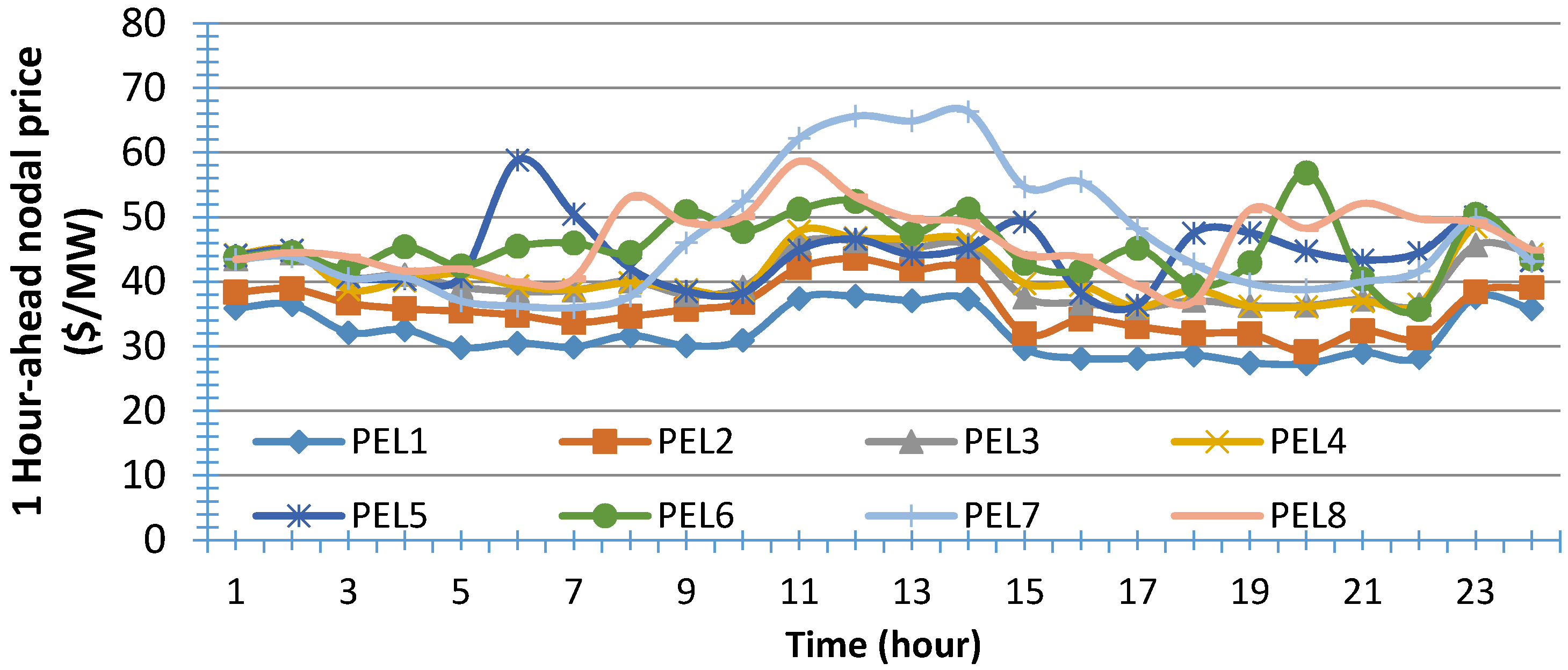
5.3. Price Elasticity Affecting Demand Response Amount

Given that wind power output fluctuation is set as Figure 2, the price elasticity of PEL 2 is changed to (−0.409, 8.3236), and other parameters of PELs are the same (Table 1). The demand response amounts of different price sensitivities are studied.

Under this scenario, the calculation results of demand response amount are shown in Figure 8, and demand response satisfaction is shown in Figure 9 and Figure 10.

Figure 8 illustrates that the expected demand response amount of PEL 2 is decreased with decrease of price elasticity coefficient. Figure 9 and Figure 10 illustrate that ECS increases when price elasticity coefficient decreases oppositely, thereby decreasing IBS. The reason is that the decrease of demand response expectation indicates that the change amount of electricity consumption manner decreases, thereby increasing ECS and decreasing IBS. These results are consistent with the analysis of the preceding conclusion.

Figure 8. Demand response amount of PEL 2 with changing α.

Figure 8. Demand response amount of PEL 2 with changing α.

Figure 9. Electricity consumption satisfaction (ECS) of PEL 2 with changing α.

Figure 9. Electricity consumption satisfaction (ECS) of PEL 2 with changing α.

Figure 10. Interaction benefit satisfaction (IBS) of PEL 2 with changing α.

Figure 10. Interaction benefit satisfaction (IBS) of PEL 2 with changing α.

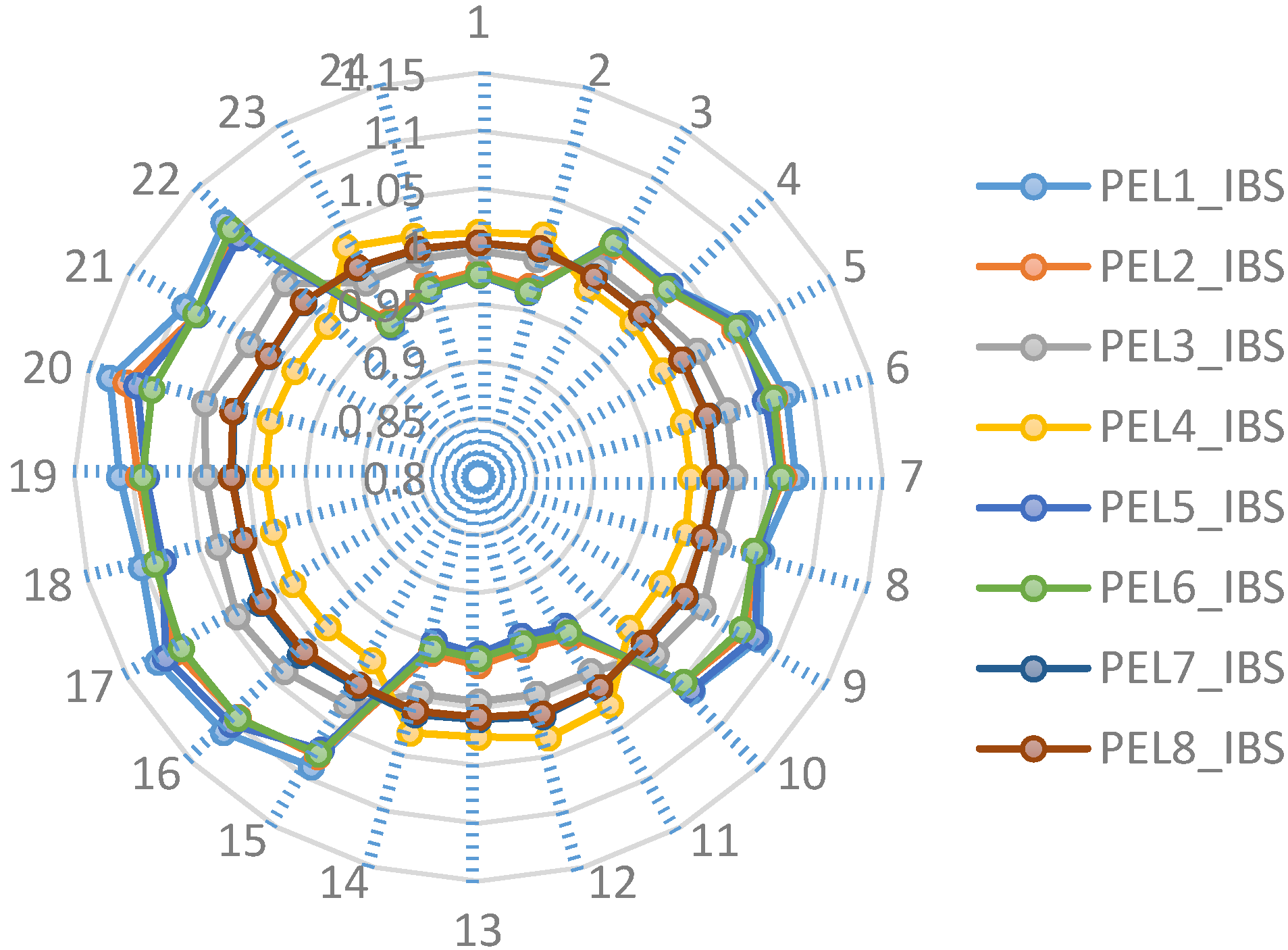
5.4. Effect of PEL Probabilistic Characterization on Demand Response Amount

If the wind power output fluctuation is set as Figure 2, the distribution coefficient k of the stochastic demand response of PEL 2 is changed to 0.3. We study the effect PEL probabilistic characterization on demand response. Other PEL parameters are the same, as shown in Table 1.

In this scenario, the demand response amount of PEL 2 is illustrated in Figure 11, and the results of demand response satisfaction are shown in Figure 12 and Figure 13.

Figure 11. Demand response Amount of PEL2 with Changing k.

Figure 11. Demand response Amount of PEL2 with Changing k.

Figure 12. Electricity consumption satisfaction (ECS) of PEL 2 with changing k.

Figure 12. Electricity consumption satisfaction (ECS) of PEL 2 with changing k.

Figure 13. Interaction benefit satisfaction (IBS) of PEL 2 with changing k.

Figure 13. Interaction benefit satisfaction (IBS) of PEL 2 with changing k.

Figure 11 illustrates that the demand response amount expectation of PEL 2 increases with increasing uncertain factors. We can also draw the following two conclusions: first, ECS decreases while IBS increases with increasing uncertain factors; and second, Figure 8 and Figure 11 have different changing trends because the price sensitivity and price elasticity coefficient are large for a large distribution coefficient of PEL stochastic demand response. Hence, a large k or high |α| corresponds to the similar trend of demand response amount. This result demonstrates the discussion about the relationship between price elasticity coefficient and distribution coefficient of PEL’s stochastic demand response in Section 2.2. Thus, under a power shortage situation, the load has a small price elasticity coefficient, which has few demand response uncertainties, and can be chosen to participate in the interaction.

5.5. Computing Performance

To solve the problem, the stochastic constraints are transformed into deterministic constraints. The solution methodology used in this paper is the particle swarm optimization (PSO). All numerical simulations are coded in MATLAB. With iterations of PSO set to 300, the running time of each case on a provincial power system with 151 buses is approximately 2.5 min on a 2.4 GHz Windows-based laptop with 8 Gb of RAM. The simulation is fully able to meet the requirement of the hourly process.

6. Conclusions

In this paper, modeling the stochastic demand response behavior of PEL is proposed. The proposed model analyzes the demand response behavior of PEL by maximizing the electricity consumption satisfaction (ECS) and interaction benefit satisfaction (IBS) of PEL. In the proposed model, the uncertainties in wind power variability are considered. Meanwhile, the uncertainties in the stochastic process of PEL demand response to the power grid are included. The confidence intervals are introduced to transform this problem to a deterministic optimization problem. This problem is solved by the particle swarm optimization (PSO) method. The main contributions are as follows:

(1)

The output of the uncertain model contains abundant probability information. It provides practical information on how PELs actively respond to the power grid integrated with wind power, thus decreasing the effects caused by the response deviation;

(2)

The relationship between the elasticity coefficient of PELs and the distribution coefficient of the stochastic demand response is elaborated. The increasing elasticity coefficient of PELs, i.e., decreasing flexibility, leads to a large distribution coefficient of stochastic demand;

(3)

Choosing PELs with small sensitivity to the price elasticity coefficient into the interaction with the power grid reduce the uncertainty and enhance reliability,

(4)

Proper choice of the distribution coefficient of ECS for PELs increases the comprehensive satisfaction of demand responses,

(5)

The proposed model enables demand response resources to respond to wind power variability. It also contributes to mitigating power imbalance, and consideration of the interaction profit with the power grid is presented; and

(6)

This approach is applicable in hourly real-time pricing models, and also in day-ahead pricing models.

References

1. Mark, Z.J.; Cristina, L.A. Saturation Wind Power Potential and Its Implications for Wind Energy. 25 September 2012. Available online: http://www.pnas.org/content/109/39/15679.full (accessed on 15 August 2014).
2. Yao, J.G.; Yang, S.C.; Wang, K.; Yang, Z.; Song, X. Concept and Research Framework of Smart Grid “Source-Grid-Load” Interactive Operation and Control. Autom. Electr. Power Syst. 2012, 36, 1–6. [Google Scholar]
3. Wang, Q.; Guan, Y.; Wang, J. A chance-constrained two-stage stochastic program for unit commitment with uncertain wind power output. IEEE Trans. Power Syst. 2012, 27, 206–215. [Google Scholar] [CrossRef]
4. Bouffard, F.; Galiana, F. Stochastic security for operations planning with significant wind power generation. IEEE Trans. Power Syst. 2008, 23, 306–316. [Google Scholar] [CrossRef]
5. Wang, J.; Botterud, A.; Miranda, V.; Monteiro, C.; Sheble, G. Impact of wind power forecasting on unit commitment and dispatch. In Proceedings of the 8th International Workshop Large-Scale Integration of Wind Power into Power Systems, Bremen, Germany, 14–15 October 2009.
6. Ruiz, P.; Philbrick, C.; Zak, E.; Cheung, K.; Sauer, P. Uncertainty management in the unit commitment problem. IEEE Trans. Power Syst. 2009, 24, 642–651. [Google Scholar] [CrossRef]
7. Wang, J.; Shahidehpour, M.; Li, Z. Security-constrained unit commitment with volatile wind power generation. IEEE Trans. Power Syst. 2008, 23, 1319–1327. [Google Scholar] [CrossRef]
8. Zeng, B.; Zhang, J.; Yang, X.; Wang, J.; Dong, J.; Zhang, Y. Integrated Planning for Transition to Low-Carbon Distribution System with Renewable Energy Generation and Demand Response. IEEE Trans. Power Syst. 2014, 29, 1153–1165. [Google Scholar] [CrossRef]
9. Nikzad, M.; Mozafari, B. Reliability assessment of incentive- and priced-based demand response programs in restructured power systems. Int. J. Electr. Power Energy Syst. 2014, 56, 83–96. [Google Scholar] [CrossRef]
10. Jia, W.; Kang, C.; Chen, Q. Analysis on demand-side interactive response capability for power system dispatch in a smart grid framework. Electr. Power Syst. Res. 2012, 90, 11–17. [Google Scholar] [CrossRef]
11. Andreas, G.V.; Pandelis, N.B. Demand Response in a Real-Time Balancing Market Clearing with Pay-as-Bid Pricing. IEEE Trans. Smart Grid 2013, 4, 1966–1975. [Google Scholar]
12. Papavasiliou, A.; Oren, S.S. Large-Scale Integration of Deferrable Demand and Renewable Energy Sources. IEEE Trans. Power Syst. 2014, 29, 489–499. [Google Scholar] [CrossRef]
13. Wang, J.; Kennedy, S.W.; Kirtley, J.L. Optimization of Forward Electricity Markets Considering Wind Generation and Demand Response. IEEE Trans. Smart Grid 2014, 5, 1254–1261. [Google Scholar] [CrossRef]
14. Li, S.; Zhang, D.; Roget, A.B.; O’Neill, Z. Integrating Home Energy Simulation and Dynamic Electricity Price for Demand Response Study. IEEE Trans. Smart Grid 2014, 5, 779–788. [Google Scholar] [CrossRef]
15. Ma, O.; Alkadi, N.; Cappers, P.; Denholm, P.; Dudley, J.; Goli, S.; Hummon, M.; Kiliccote, S.; Macdonald, J.; Matson, N.; et al. Demand Response for Ancillary Services. IEEE Trans. Smart Grid 2013, 4, 1988–1995. [Google Scholar] [CrossRef]
16. Nguyen, D.T.; Negnevitsky, M.; de Groot, M. Market-Based Demand Response Scheduling in a Deregulated Environment. IEEE Trans. Smart Grid 2013, 4, 1948–1956. [Google Scholar] [CrossRef]
17. Su, C.; Kirschen, D. Quantifying the effect of demand response on electricity markets. IEEE Trans. Power Syst. 2009, 24, 1199–1207. [Google Scholar]
18. Kirschen, D. Demand-side view of electricity markets. IEEE Trans. Power Syst 2003, 18, 520–527. [Google Scholar] [CrossRef]
19. Federal Energy Regulatory Commission. Wholesale Competition in Regions with Organized Electric Markets: FERC’s Advanced Notice of Proposed Rulemaking, 22 February 2007. Available online: http://www.kirkland.com/siteFiles/Publications/C430B16C519842DE1AEB2623F7DE21D6.pdf (accessed on 12 March 2015).
20. Mortensen, R.E.; Haggerty, K.P. A Stochastic Computer Model for Heating and Cooling Loads. IEEE Trans. Power Syst. 1998, 3, 1213–1219. [Google Scholar] [CrossRef]
21. Molina-García, A.; Kessler, M.; Fuentes, J.A.; Gómez-Lázaro, E. Probabilistic Characterization of Thermostatically Controlled Loads to Model the Impact of Demand Response Programs. IEEE Trans. Power Syst. 2011, 26, 241–251. [Google Scholar] [CrossRef]
22. Sun, Y.; Elizondo, M.; Lu, S.; Fuller, J.C. The Impact of Uncertain Physical Parameters on HVAC Demand Response. IEEE Trans. Smart Grid 2014, 5, 916–923. [Google Scholar] [CrossRef]
23. Zhao, C.; Wang, J.; Watson, J.; Guan, Y. Multi-Stage Robust Unit Commitment Considering Wind and Demand Response Uncertainties. IEEE Trans. Power Syst. 2003, 28, 2708–2719. [Google Scholar] [CrossRef]
24. Navid-Azarbaijani, N. Load Model and Control of Residential Appliances; McGill University: Montreal, QC, Canada, 1996; p. 81. [Google Scholar]
25. Zhang, B.M.; Wang, S.Y.; Xiang, N.D. A linear recursive bad data identification method with real-time application to power system state estimation. IEEE Trans. Power Syst. 1992, 7, 1378–1385. [Google Scholar] [CrossRef]
26. Wu, Y.-C.; Debs, A.S.; Marsten, R.E. A direct nonlinear predictor-corrector primal-dual interior point algorithm for optimal power flows. IEEE Trans. Power Syst. 1994, 9, 876–883. [Google Scholar]