Dimensional and Geometrical Quality Enhancement in Additively Manufactured Parts: Systematic Framework and A Case Study


Abstract
:1. Introduction
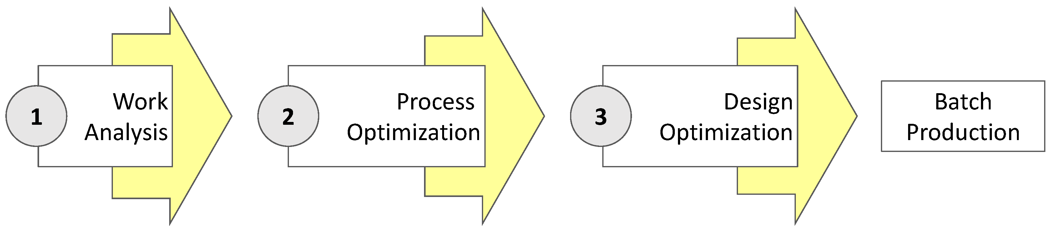
2. Systematic Framework Description
- At least one of its features is a Feature of Size. Consequently, part geometry must include at least one cylinder or two parallel opposite planes [27] affected by a dimensional tolerance;
- Batch size and part-added value justify a proportional investment of test specimens and optimization effort.
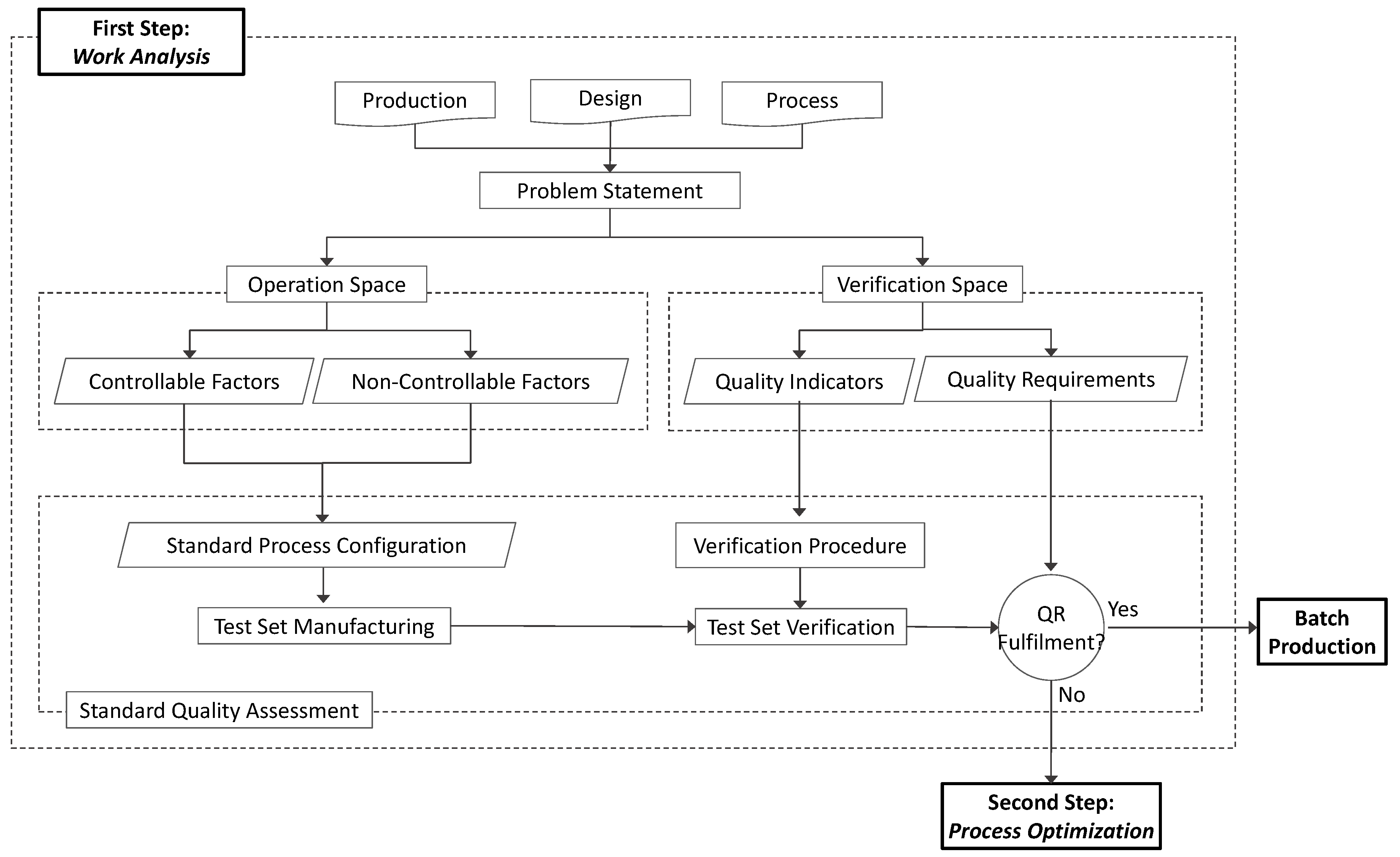
2.1. Work Analysis
- Production requirements encompass information about expected production rates, batch size, maximum profitable manufacturing cost-per-unit and all additional requirements—like expected strength or hardness—that would not be related to geometrical requirements;
- Design specifications would comprise the geometrical information of the 3D CAD file, along with dimensional and geometric tolerances requirements. Information about shapes and dimensions should be taken into account even if they are not directly affected by tolerances. Part material should also be included in this category;
- Process characteristics should include all data regarding AM processes and equipment within the scope of the problem. Depending on each particular situation, process and/or machine could be previously set or included in the problem (which implies that process would be considered as an additional factor). At the process level, staff in charge of the optimization must analyze the information about the fundamentals of the process, including physical principle, range of materials or common manufacturing defects. At the equipment level, attention should be paid to the characteristics of machines, like workspace dimensions, axes speed, operation limits, or appropriate ranges for configuration parameters (layer thickness, building speed, etc.). Batch size and part-added value justify a proportional investment on test specimens and optimization effort.
- The Operation Space would consist of all those factors that could have an influence upon part quality. This means that every single factor whose modification would presumably affect, to a certain degree, the quality of the part, must be included in the Operation Space. Factors could be subject to modification (controllable factors) or not (non-controllable factors). Controllable factors are those that can be modified according to production decisions. This category includes discrete factors (e.g., selecting “glossy” or “matte” finishing in a Material Jetting process) and continuous factors (e.g., nozzle temperature in ME of thermoplastics) that could adopt many different values within a certain range. On the other hand, non-controllable factors are those that, having an influence upon part quality, should not be modified. This category would include design decisions of requirements (shape, dimensions, material, etc.) that have been set during the design stage. It also should include production decisions (batch size, process, production machine, etc.) that are not subjected to possible modifications. Process parameters could be also considered non-controllable factors when their values have been set according to material or machine supplier recommendations, workshop procedures or workforce experience. Categorization of influence factors into non-controllable and controllable groups is a key task. Most factors undoubtedly belong to one of these groups, but special attention should be paid to those factors that do not have a significant influence upon quality according to previous know-how, since there is a risk of neglecting their influence upon a particular part or feature, despite their actual significance;
- The Verification Space would be formed by Quality Indicators (QI) and Quality Requirements (QR). QI would be used for evaluating the degree of compliance of the tolerances imposed during the design stage. They would usually match FoS quality requirements, like dimensions (diameter of a cylindrical feature or distance between parallel flat surfaces) or geometrical deviation of controlled features (flatness, parallelism, cylindricity or concentricity). Nevertheless, QI could also be defined as relative differences between those parameters and their optimal values (e.g., the difference between the measured diameter and the middle value of the tolerance interval). During the definition of QI, it would also be necessary to define the verification procedure. This means that an inspection plan should be elaborated, including the materials and methods used for verifying each part and calculating actual values for each QI. Finally, QR are defined as the range of acceptable values that each single QI should adopt to enable batch production.
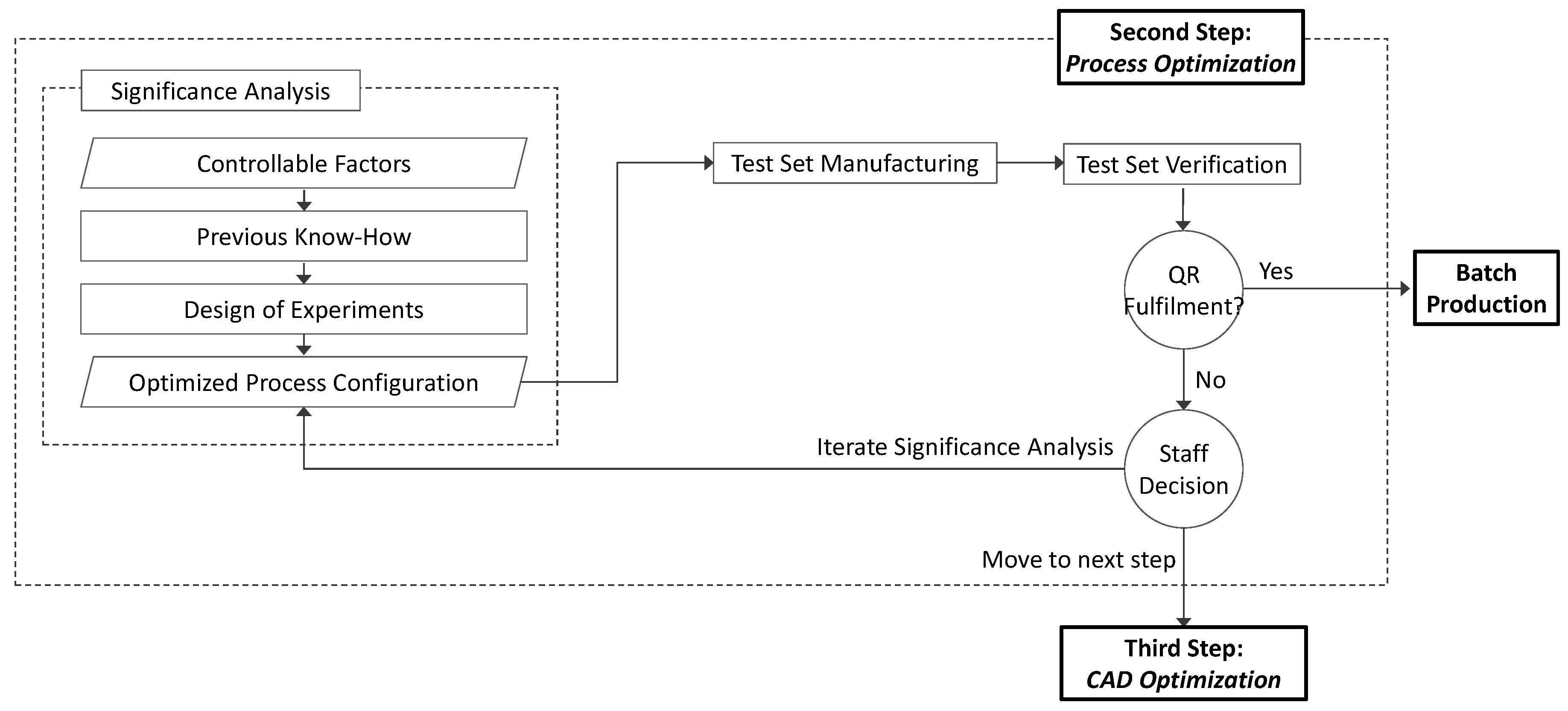
2.2. Process Optimization
2.3. Design Optimization
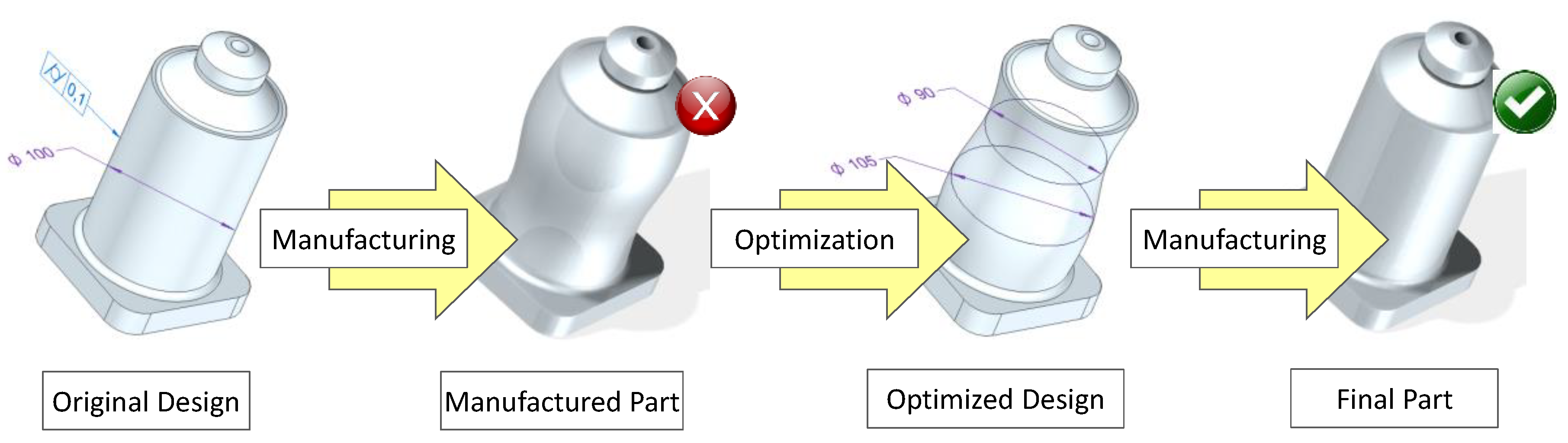
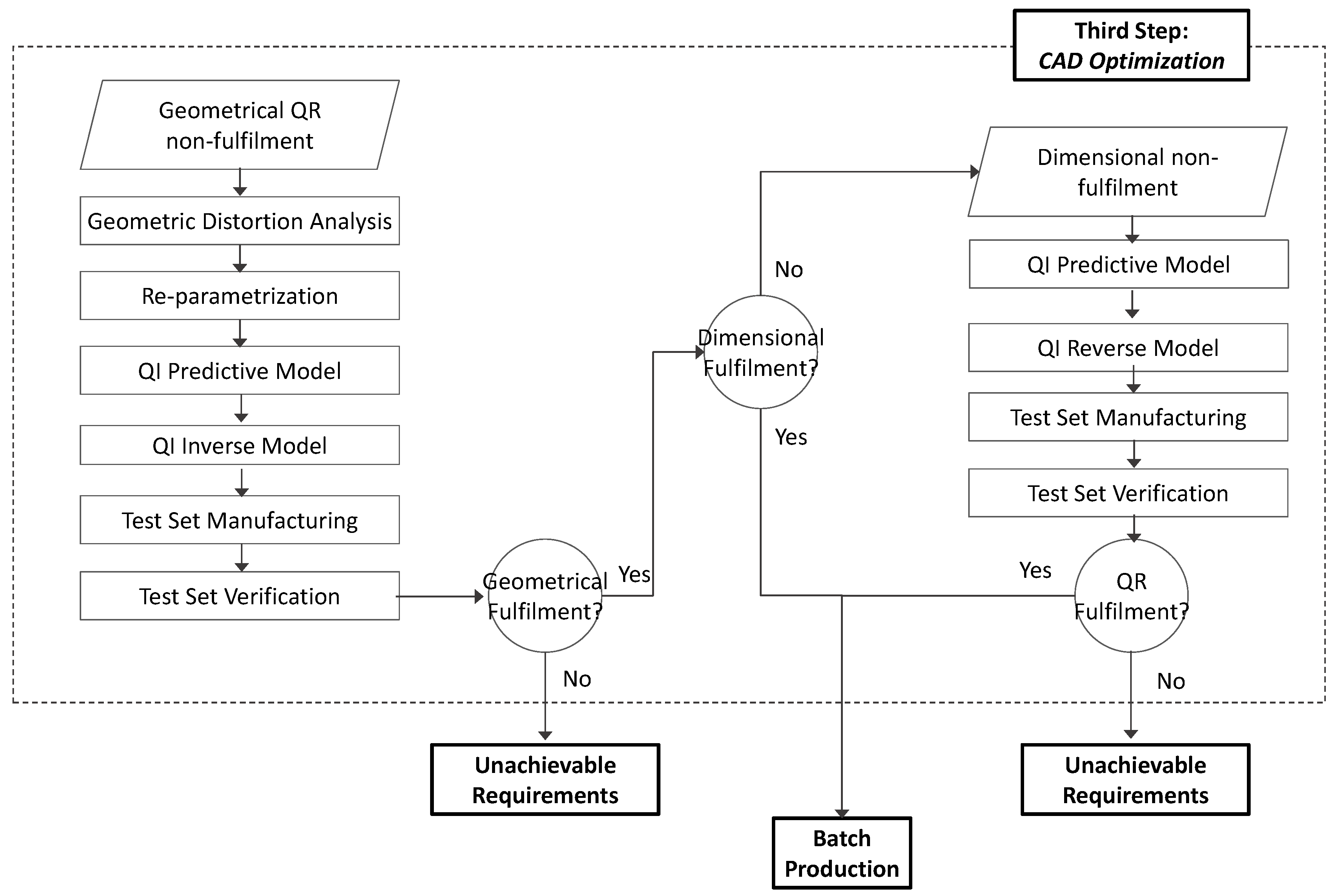
- Dimensional non-fulfilments could be corrected if the observed variability of QI is comparatively lower than the range of acceptable values defined by each correspondent QR. In these cases, Design Optimization searches for a model where the values of design parameters related to QI could be modified to improve quality. This means that optimization could be conducted without modifying the initial parameterization of the part, since only the values of existing parameters would be modified according to the correspondent inverse model;
- Geometrical non-fulfilments, on the other hand, demand the change of part parameterization at the design stage, which could be a more complex task. In this situation, a model of geometric distortion would be necessary. The ideal situation at this point is that analysis of part geometric distortion leads to a recognizable pattern that could be easily parameterized—e.g., if a theoretically cylindrical feature resembles an elliptic cylinder once manufactured, the geometric distortion model should determine the orientation of the major and minor axis, and the correspondent equation coefficients and re-parameterization turns, to be almost direct. Nevertheless, in other situations, modelling the deformed geometry would require methods of higher complexity. E.g., if the deformation does not resemble any common primitive, the theoretical cylinder could be modelled by means of a free-form adjustment based on Non-Uniform Rational Basis Splines (NURBS). Research efforts should be conducted in order to select the most appropriate fitting model, minimizing as much as possible the model complexity and taking into account each particular CAD suite capability for manipulating different types of parameterization. In both cases, original parameterization should be substituted with a new parameterization that follows actual manufactured geometries. Once this objective is achieved, the problem is similar to that described for dimensional non-fulfillments (defining a predictive model and an inverse model) with the difference that, in this case, alternative design parameters are used.
2.4. Practical Recommendations
- Optimization steps should be carried out using the minimal number of experiments and also minimizing the number of test specimens that would be manufactured;
- Subjective decisions regarding process configuration should be avoided whenever possible;
- Several tasks could have an iterative application when results suggest that additional research could be worthwhile;
- Factors categorized as non-controllable by following previous know-how or good-practices recommendations could have a more significant influence than previously thought for certain geometries. Accordingly, if QI variance could not be put under control by means of controllable-factor adjustment, such categorizations must be carefully revised.
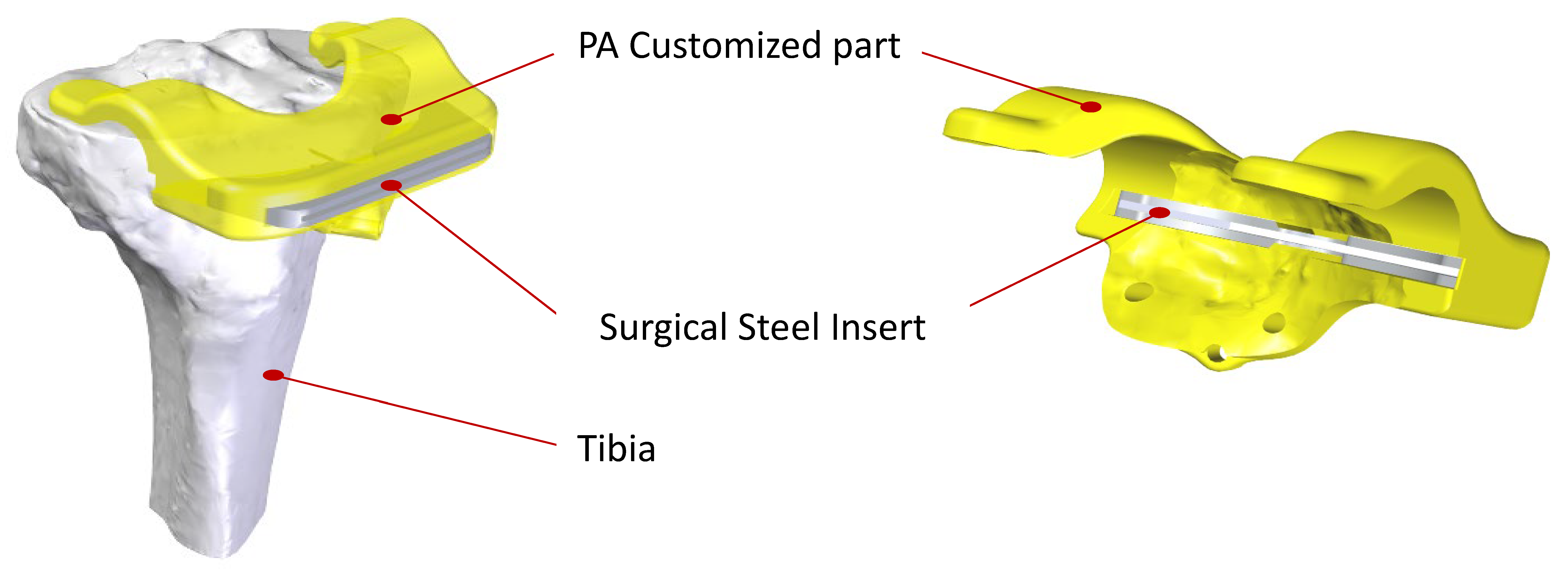
3. Case Study: Optimization of Surgical-Steel Tibia Resection Guides
3.1. Step 1: Work Analysis
3.1.1. Operation Space
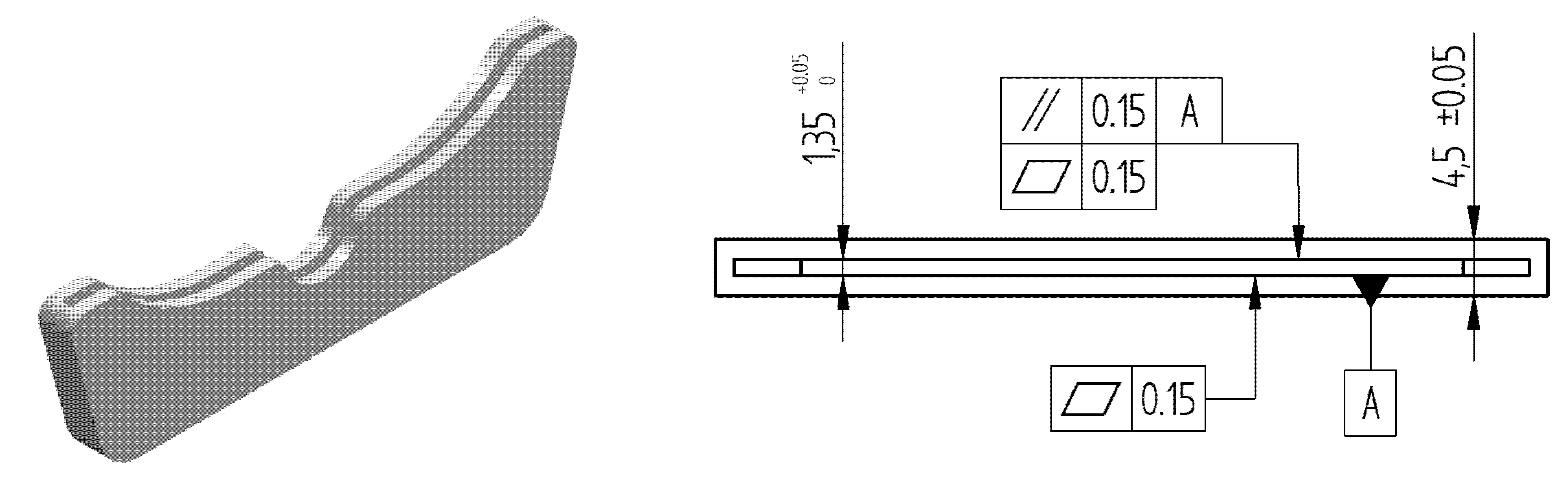
3.1.2. Verification Space
3.1.3. Standard Quality Assessment
3.2. Step 2: Process Optimization
- Layer Thickness value was set during the Standard Quality Assessment at the minimum achievable level (20 µm). Delgado et al. [31] have not found a statistically significant effect of Layer Thickness upon dimensional error in L-PBF for test specimens with non-sloped surfaces (like the one analyzed in the present work). On the other hand, Nguyen et al. [32] reported an increase in dimensional accuracy with decreasing layer thickness, and this result seems to have been confirmed by Maamoun et al. [33]. Although it is sometimes difficult to compare results, no research has been found supporting the hypothesis that thicker layers could improve dimensional quality. Accordingly, since the minimum achievable value for Layer Thickness has already been used for the Standard Process Configuration, this factor should not be included during the Process Optimization step;
- Sand blasting is the usual finishing process in L-PBF, since it is intended to remove metallic projections that appear as spikes on part surfaces. Consequently, sand blasting is presumed to reduce the unevenness of surfaces. This means that suppressing sand blasting would probably cause an increment in flatness and parallelism deviations and also could affect dimensional quality. These arguments led to the consideration of sand blasting as an unavoidable step;
- Part location within the working area could influence quality results, and this hypothesis could be tested using data from the previous step. Analyzing how DS measures are related to part location within the trays, the Pearson Correlation provides a p-value of 0.721. This value reveals an extremely low probability of a linear relationship between DS and part location for the standard process configuration. Additionally, none of the other indicators (FSR, FSF, PS and DE) show any correlation with part location according to their p-values. This means that variability in QI cannot be explained by part location within the tray, and, thus, modifying location would not allow for fulfilment of QR;
- Lightweight supporting structures were preferred during the Standard Quality Assessment because part removal was easier and did not demand subsequent machining. Nevertheless, manual removal of support could have an influence upon observed lack of quality [34], so Type of Support should be included as a possible influence factor in the Process Optimization step;
- Similarly, thermal stresses accumulated during manufacturing operations (in-layer and layer-upon-layer) could provoke a noticeable distortion in the part, after they are released from support [35]. Accordingly, thermal treatment should be included in the Process Optimization step.
3.3. Step 3: Design Optimization
3.3.1. Predictive and Inverse Models
- Design values for DS will be thereafter denoted as DSD, whereas the correspondent values measured after part manufacturing will be denoted DSM. Equivalent notation will be used for DED and DEM;
- Modifying DSD could not only affect DSM, but also DEM and, vice versa, modifying DED could have and influence upon DSM;
- Predictive model should include design factor (DSD) as part of its parameterization. To achieve better results, the set of data that would be used to adjust such models should also include variations in design factors.
3.3.2. Optimized Design Quality Assessment
4. Discussion
5. Conclusions
Author Contributions
Funding
Acknowledgments
Conflicts of Interest
References
- Additive Manufacturing—General Principles—Part 1: Terminology; ISO/DIS 17296-1; International Organization for Standardization: Genève, Switzerland, 2014.
- Standard Terminology for Additive Manufacturing Technologies; ASTM F2792-12; ASTM International: West Conshohocken, PA, USA, 2012.
- Basiliere, P.; Shanler, M. Hype Cycle for 3D Printing; Gartner Inc.: Stamford, CT, USA, 2019. [Google Scholar]
- Wohlers, T. Wohlers Report 2012—Additive Manufacturing and 3D Printing State of the Industry: Annual Worldwide Progress Report; Wohlers Associates: Fort Collins, CO, USA, 2012. [Google Scholar]
- Feenstra, F. Additive Manufacturing: SASAM Standardisation Roadmap 2014. Available online: https://www.rm-platform.com/downloads2/send/2-articles-publications/607-sasam-standardisation-roadmap-2014 (accessed on 7 September 2019).
- Masood, S.H.; Rattanawong, W.; Iovenitti, P. Part build orientations based on volumetric error in fused deposition modeling. Int. J. Adv. Manuf. Tech. 2000, 16, 162–168. [Google Scholar] [CrossRef]
- Noriega, A.; Blanco, D.; Alvarez, B.J.; Garcia, A. Dimensional Accuracy Improvement of FDM Square Cross-Section Parts Using Artificial Neural Networks and an Optimization Algorithm. Int. J. Adv. Manuf. Tech. 2013, 69, 2301–2313. [Google Scholar] [CrossRef]
- Boschetto, A.; Bottini, L. Triangular mesh offset aiming to enhance Fused Deposition Modeling accuracy. Int. J. Adv. Manuf. Tech. 2015, 80, 99–111. [Google Scholar] [CrossRef]
- Armillotta, A.; Bellotti, M.; Cavallaro, M. Warpage of FDM parts: Experimental tests and analytic model. Robot. CIM Int. Manuf. 2018, 50, 140–152. [Google Scholar] [CrossRef]
- Ikeuchi, D.; Vargas-Uscategui, A.; Wu, X.; King, P.C. Neural Network Modelling of Track Profile in Cold Spray Additive Manufacturing. Materials 2019, 12, 2827. [Google Scholar] [CrossRef] [PubMed]
- Chang, D.Y.; Huang, B.H. Studies on profile error and extruding aperture for the RP parts using the fused deposition modelling process. Int. J. Adv. Manuf. Technol. 2011, 53, 1027–1037. [Google Scholar] [CrossRef]
- Brajlih, T.; Valentan, B.; Balic, J.; Drstvensek, I. Speed and accuracy evaluation of additive manufacturing machines. Rapid Prototyp. J. 2011, 17, 64–75. [Google Scholar] [CrossRef]
- El-Katatny, I.; Masood, S.H.; Morsi, Y.S. Error analysis of FDM fabricated medical replicas. Rapid Prototyp. J. 2010, 16, 36–43. [Google Scholar] [CrossRef]
- Byun, H.S.; Lee, K.H. Determination of the optimal build direction for different rapid prototyping processes using multi-criterion decision making. Robot. CIM Int. Manuf. 2006, 22, 69–80. [Google Scholar] [CrossRef]
- Lee, B.H.; Abdullah, J.; Khan, Z.A. Optimization of rapid prototyping parameters for production of flexible ABS object. J. Mater. Process. Technol. 2005, 169, 54–61. [Google Scholar] [CrossRef]
- Kumar, V.V.; Tagore, G.R.N.; Venugopal, A. Some investigations on geometric conformity analysis of a 3-D freeform objects produced by rapid prototyping (FDM) process. Int. J. Appl. Res. Mech. Eng. 2011, 1, 82–86. [Google Scholar]
- Tong, K.; Joshi, S.; Lehtinet, E.A. Error compensation for fused deposition modeling (FDM) machine by correcting slice files. Rapid Prototyp. J. 2008, 14, 4–14. [Google Scholar] [CrossRef]
- Sood, A.K. Study on Parametric Optimization of Used Deposition Modelling (FDM) Process. Ph.D. Thesis, National Institute of Technology, Rourkela, India, 2011. [Google Scholar]
- Baturynskaa, I.; Semeniuta, O.; Martinsen, K. Optimization of process parameters for powder bed fusion additive manufacturing by combination of machine learning and finite element method: A conceptual framework. Procedia CIRP 2018, 67, 227–232. [Google Scholar] [CrossRef]
- Zhu, Z.; Answer, N.; Huang, Q.; Mathieu, L. Machine learning in tolerancing for additive manufacturing. CIRP Ann. Manuf. Technol. 2018, 67, 157–160. [Google Scholar] [CrossRef]
- Shen, Z.; Shang, X.; Li, Y.; Bao, Y.; Zhang, X.; Dong, X.; Wan, L.; Xiong, G.; Wang, F.Y. PredNet and CompNet: Prediction and High-Precision Compensation of In-Plane Shape Deformation for Additive Manufacturing. In Proceedings of the 2019 IEEE 15th International Conference on Automation Science and Engineering (CASE), Vancouver, BC, Canada, 22–26 August 2019. [Google Scholar] [CrossRef]
- Chowdhury, S.; Anand, S. Artificial Neural Network Based Geometric Compensation for Thermal Deformation in Additive Manufacturing Processes. In Proceedings of the ASME 2016 11th International Manufacturing Science and Engineering Conference (MSEC 2016), Blacksburg, VA, USA, 27 June–1 July 2016. [Google Scholar] [CrossRef]
- Paul, R. Modeling and Optimization of Powder Based Additive Manufacturing (AM) Processes. Ph.D. Thesis, University of Cincinnati, Cincinnati, OH, USA, 2013. [Google Scholar]
- Moroni, G.; Syam, W.P.; Petrò, S. Towards early estimation of part accuracy in additive manufacturing. Procedia CIRP 2014, 21, 300–305. [Google Scholar] [CrossRef]
- Liu, X.; Liu, L.; Zhao, Y.; Ma, J.; Meng, L.I.; Mao, L. Optimization of Forming Accuracy of Additive Manufacturing Complex Parts Based on PSO. In Proceedings of the 14th IEEE Conference on Industrial Electronics and Applications (ICIEA), Xi’an, China, 19–21 June 2019. [Google Scholar] [CrossRef]
- Moylan, S.; Brown, C.U.; Slotwinski, J. Recommended Protocol for Round Robin Studies in Additive Manufacturing. J. Test. Eval. 2016, 44, 1009–1018. [Google Scholar] [CrossRef]
- General Tolerances. Part 1: Tolerances for Linear and Angular Dimensions without Individual Tolerance Indications; ISO 2768-1; International Organization for Standardization: Genève, Switzerland, 1989. [Google Scholar]
- Montgomery, D.C. Design and Analysis of Experiments, 9th ed.; John Wiley & Sons: Hoboken, NJ, USA, 2017. [Google Scholar]
- Surgical Operations and Procedures Performed in Hospitals (Eurostat). Available online: http://ec.europa.eu/eurostat/statistics-explained/images/0/06/Surgical_operations_and_procedures_Health2015B.xlsx (accessed on 21 September 2019).
- Gibson, I.; Rosen, D.W.; Stucker, B. Additive Manufacturing Technologies. Rapid Prototyping to Direct Digital Manufacturing; Springer: New York, NY, USA, 2010. [Google Scholar]
- Delgado, J.; Ciurana, J.; Rodríguez, C.A. Influence of process parameters on part quality and mechanical properties for DMLS and SLM with iron-based materials. Int. J. Adv. Manuf. Technol. 2012, 60, 601–610. [Google Scholar] [CrossRef]
- Nguyen, B.; Luu, D.N.; Nai, S.M.L.; Zhu, Z.; Chen, Z.; Wei, J. The role of powder layer thickness on the quality of SLM printed parts. Arch. Civ. Mech. Eng. 2018, 18, 948–955. [Google Scholar] [CrossRef]
- Maamoun, A.H.; Xue, Y.F.; Elbestawi, M.A.; Veldhuis, S.C. Effect of Selective Laser Melting Process Parameters on the Quality of Al Alloy Parts: Powder Characterization, Density, Surface Roughness, and Dimensional Accuracy. Materials 2018, 11, 2343. [Google Scholar] [CrossRef]
- Järvinen, J.-P.; Matilainen, V.; Li, X.; Piili, H.; Salminen, A.; Mäkelä, I.; Nyrhilä, O. Characterization of effect of support structures in laser additive manufacturing of stainless steel. Phys. Procedia 2014, 56, 72–81. [Google Scholar] [CrossRef]
- Mercelis, P.; Kruth, J.P. Residual stresses in selective laser sintering and selective laser melting. Rapid Prototyp. J. 2006, 12, 254–265. [Google Scholar] [CrossRef]


| Category | Factor–Level 1 | Factor–Level 2 | Controllable | Non-Controllable |
|---|---|---|---|---|
| Production | ||||
| Batch Size | X | |||
| Type of process | X | |||
| Equipment | X | |||
| Design | ||||
| Geometry | X | |||
| Dimensions | X | |||
| Material | X | |||
| Process | ||||
| Process Parameters | ||||
| Layer Thickness | X | |||
| Volume Rate | X | |||
| Scan Speed | X | |||
| Power | X | |||
| Ambient Parameters | X | |||
| Base Temperature | X | |||
| Part Orientation | X | |||
| Part Location | X | |||
| Type of Support | X | |||
| Post-Processing | ||||
| Support Removal | X | |||
| Thermal/Heat Treatment | X | |||
| Sand Blasting | X |
| Priority Order | QI | Lower Limit (mm) | Upper Limit (mm) |
|---|---|---|---|
| 1 | DS | 1.350 | 1.400 |
| 2 | FSR | - | 0.150 |
| 3 | FSF | - | 0.150 |
| 4 | PS | - | 0.150 |
| 5 | DE | 4.450 | 4.550 |
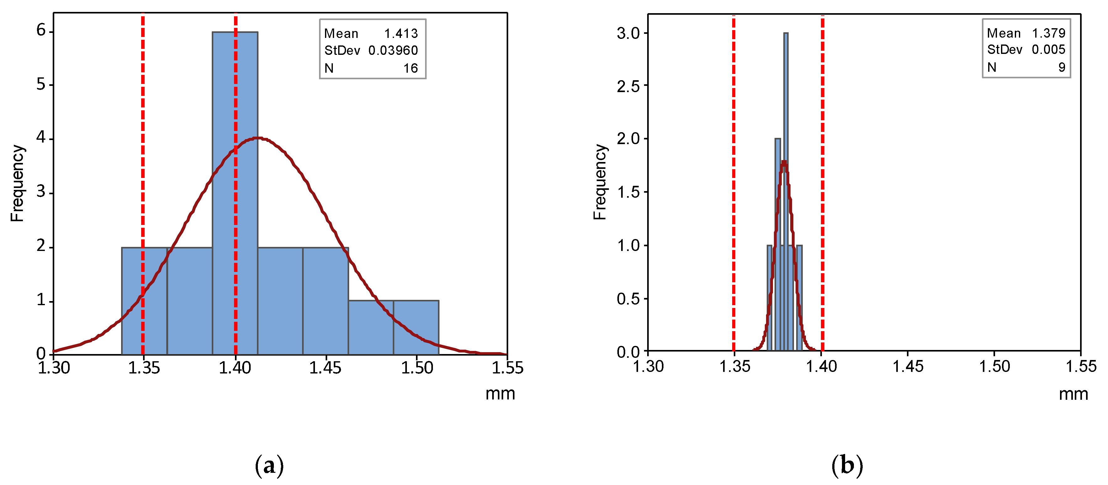
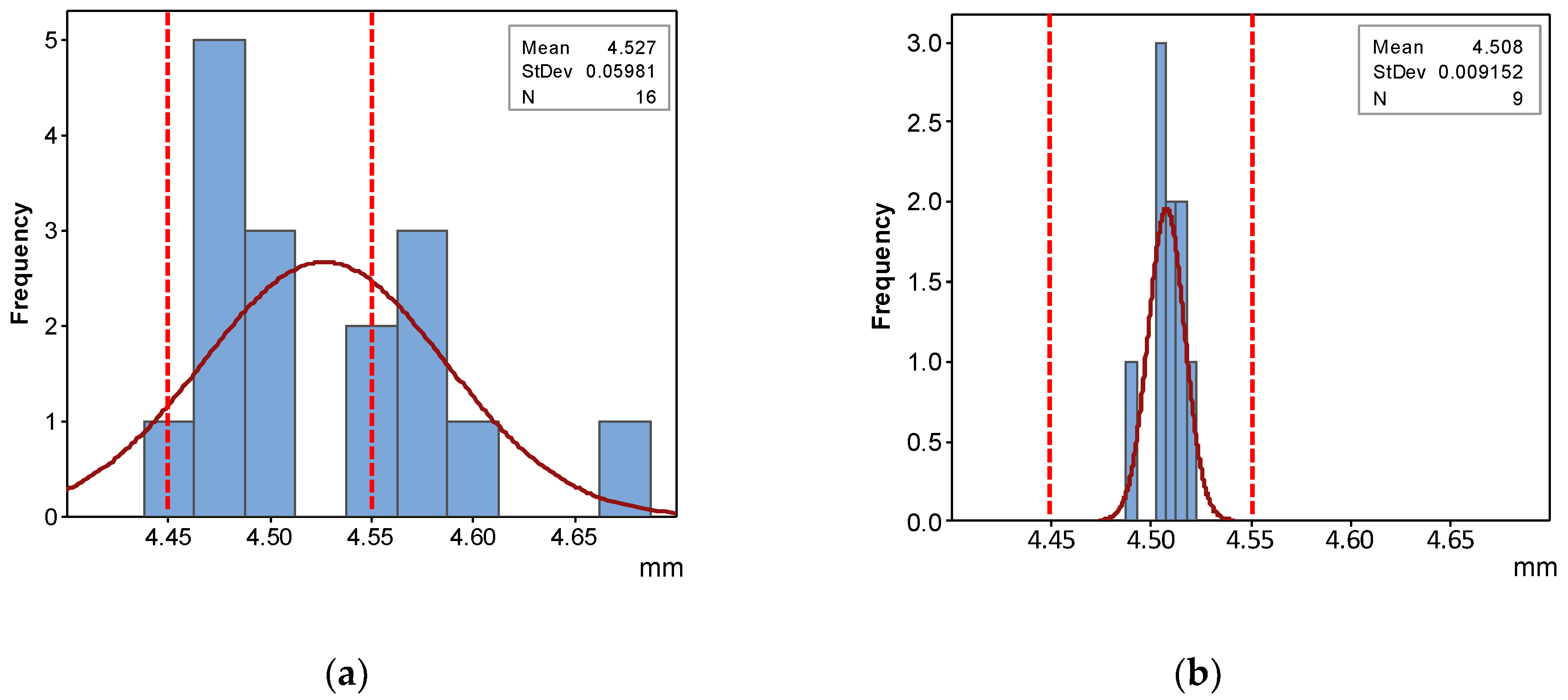
| Item | Tray | Location | DS (mm) | FSR (mm) | FSF (mm) | PS (mm) | DE (mm) |
|---|---|---|---|---|---|---|---|
| 1 | 01 | 1 | 1.359 | 0.135 | 0.266 | 0.278 | |
| 2 | 01 | 2 | 1.378 | 0.188 | 0.113 | 0.193 | 4.504 |
| 3 | 01 | 3 | 1.398 | 0.121 | 0.378 | 0.382 | 4.572 |
| 4 | 01 | 4 | 1.405 | 0.160 | 0.331 | 0.406 | 4.561 |
| 5 | 02 | 1 | 1.450 | 0.140 | 0.275 | 0.374 | 4.555 |
| 6 | 02 | 2 | 1.400 | 0.177 | 0.109 | 0.219 | 4.477 |
| 7 | 02 | 3 | 1.397 | 0.120 | 0.103 | 0.209 | 4.467 |
| 8 | 02 | 4 | 1.440 | 0.317 | 0.127 | 0.425 | 4.600 |
| 9 | 03 | 1 | 1.429 | 0.123 | 0.397 | 0.435 | 4.568 |
| 10 | 03 | 2 | 1.396 | 0.125 | 0.167 | 0.194 | 4.479 |
| 11 | 03 | 3 | 1.381 | 0.141 | 0.170 | 0.189 | 4.453 |
| 12 | 03 | 4 | 1.495 | 0.295 | 0.137 | 0.469 | 4.572 |
| 13 | 04 | 1 | 1.485 | 0.338 | 0.257 | 0.636 | 4.668 |
| 14 | 04 | 2 | 1.359 | 0.120 | 0.190 | 0.201 | 4.482 |
| 15 | 04 | 3 | 1.424 | 0.116 | 0.076 | 0.193 | 4.489 |
| 16 | 04 | 4 | 1.405 | 0.112 | 0.128 | 0.148 | 4.487 |
| Average (mm) | 1.413 | 0.171 | 0.201 | 0.309 | 4.527 | ||
| Standard Deviation (mm) | 0.040 | 0.076 | 0.103 | 0.140 | 0.060 | ||
| QR Fulfilment | 43.7% | 62.2% | 43.7% | 6.25% | 56.2% |
| ID | DS (mm) | FSR (mm) | FSF (mm) | PS (mm) | DE (mm) |
|---|---|---|---|---|---|
| Average | 1.427 | 0.095 | 0.077 | 0.096 | 4.456 |
| Standard Deviation | 0.009 | 0.013 | 0.016 | 0.011 | 0.012 |
| QR Fulfilment | 0% | 100% | 100% | 100% | 75% |
| ID | X | Y | DS (mm) | FSR (mm) | FSF (mm) | PS (mm) | DE (mm) |
|---|---|---|---|---|---|---|---|
| 1 | −1 | −1 | 1.431 | 0.080 | 0.091 | 0.108 | 4.454 |
| 2 | −1 | 1 | 1.426 | 0.117 | 0.062 | 0.084 | 4.432 |
| 3 | 0 | 0 | 1.421 | 0.078 | 0.057 | 0.070 | 4.458 |
| 4 | 0 | 0 | 1.423 | 0.089 | 0.082 | 0.089 | 4.453 |
| 5 | 1 | −1 | 1.413 | 0.086 | 0.092 | 0.103 | 4.458 |
| 6 | 1 | 1 | 1.420 | 0.096 | 0.062 | 0.088 | 4.466 |
| 7 | −1 | −1 | 1.443 | 0.094 | 0.084 | 0.105 | 4.450 |
| 8 | −1 | 1 | 1.433 | 0.085 | 0.090 | 0.097 | 4.473 |
| 9 | 0 | 0 | 1.428 | 0.088 | 0.077 | 0.080 | 4.452 |
| 10 | 0 | 0 | 1.428 | 0.092 | 0.083 | 0.101 | 4.455 |
| 11 | 1 | −1 | 1.424 | 0.092 | 0.083 | 0.101 | 4.461 |
| 12 | 1 | 1 | 1.423 | 0.110 | 0.052 | 0.078 | 4.457 |
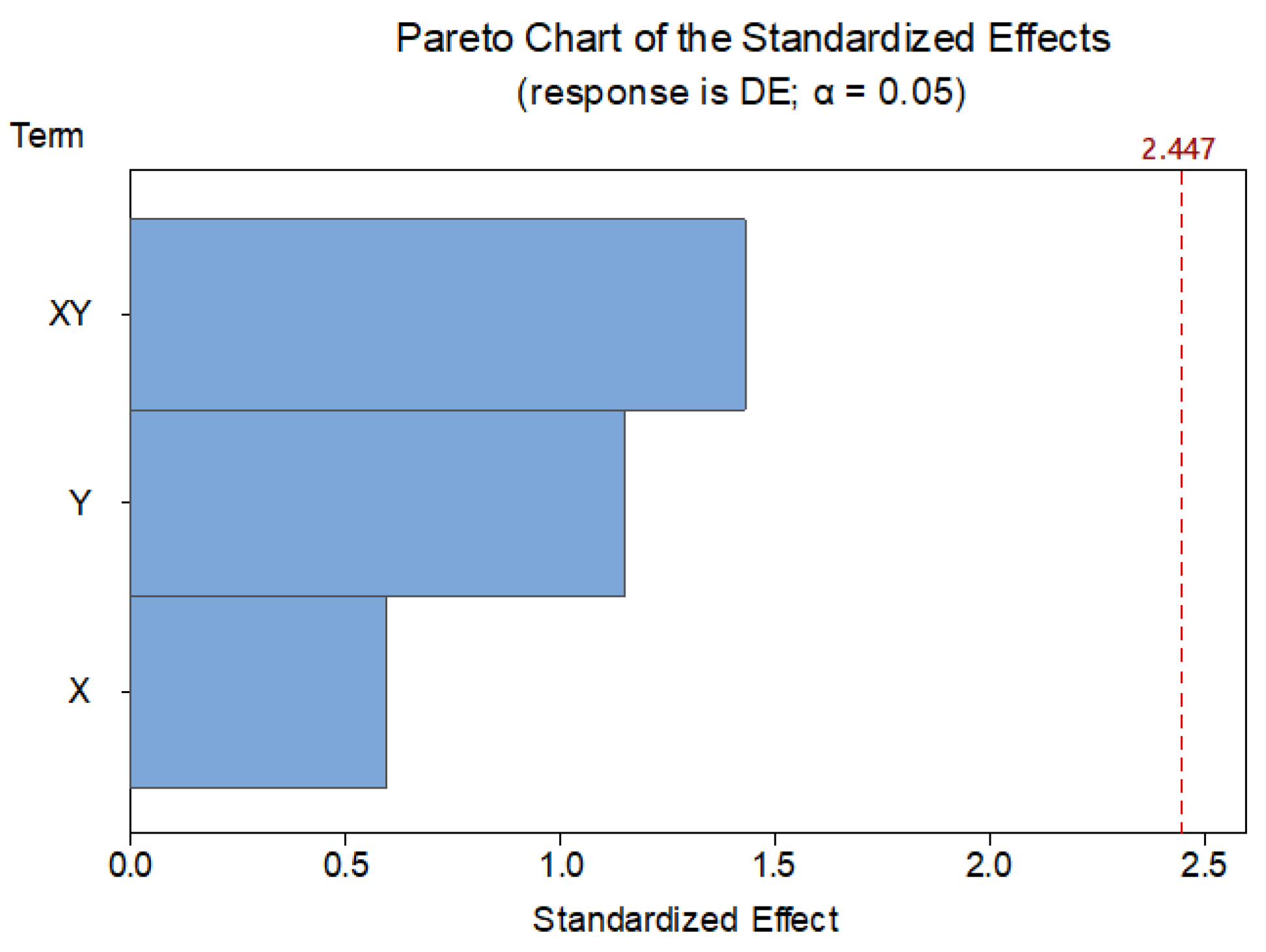
| Source | DF | Adj SS | Adj MS | f-Value | p-Value |
|---|---|---|---|---|---|
| Model | 5 | 0.000592 | 0.000118 | 23.11 | 0.001 |
| Blocks | 1 | 0.000169 | 0.000169 | 32.93 | 0.001 |
| Linear | 2 | 0.000361 | 0.000181 | 35.24 | 0.000 |
| X | 1 | 0.000351 | 0.000351 | 68.51 | 0.000 |
| Y | 1 | 0.00001 | 0.00001 | 1.98 | 0.209 |
| 2-Way Interactions | 1 | 0.000055 | 0.000055 | 10.76 | 0.017 |
| X*Y | 1 | 0.000055 | 0.000055 | 10.76 | 0.017 |
| Curvature | 1 | 0.000007 | 0.000007 | 1.37 | 0.286 |
| Error | 6 | 0.000031 | 0.000005 | ||
| Lack-of-Fit | 4 | 0.000029 | 0.000007 | 7.19 | 0.126 |
| Pure Error | 2 | 0.000002 | 0.000001 | ||
| Total | 11 | 0.000623 | |||
| Model Summary | |||||
| S | R-sq | R-sq(adj) | R-sq(pred) | ||
| 0.0022638 | 95.06% | 90.95% | 73.96% |
| ID | X (mm) | Y (mm) | DSD (mm) | DSM (mm) |
|---|---|---|---|---|
| 1 | −77.25 | −90.58 | 1.25 | 1.311 |
| 2 | −77.25 | 90.58 | 1.25 | 1.307 |
| 3 | −12.25 | 0 | 1.25 | 1.329 |
| 4 | 12.25 | 0 | 1.25 | 1.331 |
| 5 | 77.25 | −90.58 | 1.25 | 1.319 |
| 6 | 77.25 | 90.58 | 1.25 | 1.306 |
| 7 | −77.25 | −90.58 | 1.35 | 1.437 |
| 8 | −77.25 | 90.58 | 1.35 | 1.430 |
| 9 | −12.25 | 0 | 1.35 | 1.424 |
| 10 | 12.25 | 0 | 1.35 | 1.426 |
| 11 | 77.25 | −90.58 | 1.35 | 1.418 |
| 12 | 77.25 | 90.58 | 1.35 | 1.421 |
| Coefficient | Estimated Value |
|---|---|
| a1 | −4.32500 × 10⁻² |
| a2 | −3.25450 × 10⁻⁵ |
| a3 | −2.89799 × 10⁻⁵ |
| a4 | 1.08833 × 10−0 |
| ID | X (mm) | Y (mm) | DSO (mm) | DSM (mm) | DEO (mm) | DEM (mm) |
|---|---|---|---|---|---|---|
| 1 | −77.25 | −90.58 | 1.298 | 1.374 | 4.543 | 4.507 |
| 2 | −77.25 | 90.58 | 1.303 | 1.378 | 4.543 | 4.508 |
| 3 | −38.625 | −45.29 | 1.301 | 1.383 | 4.543 | 4.506 |
| 4 | −38.625 | 45.29 | 1.303 | 1.380 | 4.543 | 4.503 |
| 5 | 0 | 0 | 1.303 | 1.371 | 4.543 | 4.488 |
| 6 | 38.625 | −45.29 | 1.303 | 1.374 | 4.543 | 4.508 |
| 7 | 38.625 | 45.29 | 1.305 | 1.380 | 4.543 | 4.514 |
| 8 | 77.25 | −90.58 | 1.303 | 1.381 | 4.543 | 4.514 |
| 9 | 77.25 | 90.58 | 1.308 | 1.387 | 4.543 | 4.521 |
© 2019 by the authors. Licensee MDPI, Basel, Switzerland. This article is an open access article distributed under the terms and conditions of the Creative Commons Attribution (CC BY) license (http://creativecommons.org/licenses/by/4.0/).
Share and Cite
Beltrán, N.; Blanco, D.; Álvarez, B.J.; Noriega, Á.; Fernández, P. Dimensional and Geometrical Quality Enhancement in Additively Manufactured Parts: Systematic Framework and A Case Study. Materials 2019, 12, 3937. https://doi.org/10.3390/ma12233937
Beltrán N, Blanco D, Álvarez BJ, Noriega Á, Fernández P. Dimensional and Geometrical Quality Enhancement in Additively Manufactured Parts: Systematic Framework and A Case Study. Materials. 2019; 12(23):3937. https://doi.org/10.3390/ma12233937
Chicago/Turabian StyleBeltrán, Natalia, David Blanco, Braulio José Álvarez, Álvaro Noriega, and Pedro Fernández. 2019. "Dimensional and Geometrical Quality Enhancement in Additively Manufactured Parts: Systematic Framework and A Case Study" Materials 12, no. 23: 3937. https://doi.org/10.3390/ma12233937