DDC Control Techniques for Three-Phase BLDC Motor Position Control


1
College of Automation, Nanjing University of Aeronautics and Astronautics, Nanjing 210016, China
2
College of Information Science and Technology, Donghua University, Shanghai 201620, China
*
Author to whom correspondence should be addressed.
Algorithms 2017, 10(4), 110; https://doi.org/10.3390/a10040110
Submission received: 30 June 2017
/
Revised: 18 September 2017
/
Accepted: 18 September 2017
/
Published: 25 September 2017
Abstract
:In this article, a novel hybrid control scheme is proposed for controlling the position of a three-phase brushless direct current (BLDC) motor. The hybrid controller consists of discrete time sliding mode control (SMC) with model free adaptive control (MFAC) to make a new data-driven control (DDC) strategy that is able to reduce the simulation time and complexity of a nonlinear system. The proposed hybrid algorithm is also suitable for controlling the speed variations of a BLDC motor, and is also applicable for the real time simulation of platforms such as a gimbal platform. The DDC method does not require any system model because it depends on data collected by the system about its Inputs/Outputs (IOS). However, the model-based control (MBC) method is difficult to apply from a practical point of view and is time-consuming because we need to linearize the system model. The above proposed method is verified by multiple simulations using MATLAB Simulink. It shows that the proposed controller has better performance, more precise tracking, and greater robustness compared with the classical proportional integral derivative (PID) controller, MFAC, and model free learning adaptive control (MFLAC).
1. Introduction
In the past two decades, the brushless direct current motor has played a vital role in industrial development. These motors are widely used in industrial applications because of their better architecture that is quite suitable for many critical tasks [1,2]. The rapid development of BLDC motors in the automobile industry, based on hybrid drives that require higher efficiency permanent magnet motor (PMM) drives, was the establishment of awareness in BLDC motors [3,4]. These motors have a linear relationship between torque, current, and voltage, and they operate on a revolution per minute (RPM) basis.
A BLDC motor has the same speed torque curve as a conventional permanent magnet DC motor. However, it has different advantages, such as a small volume, a quick dynamic response, greater power density, better efficiency, and it can be directly associated with the mechanical load [5,6,7]. The BLDC motor does not use brushes, and it has extended operating life without noise. Moreover, it has Permanent Magnet, which is why its ratio is quite a bit higher between torque and motor size and is quite suitable for that application where weight and space are significant. It has a variety of speed ranges, better torque and speed characteristics as compared to other motors, and it is more suitable for applications such as a gimbal platform. However, in this research, the BLDC motor is chosen due to its low inertia in the rotor that helps to improve its acceleration time when it is operating for a short period of time [8].
In this research, a BLDC motor is selected as compared to a DC servo motor because it has many problems, such as maintenance and durability issues and higher noise. On the other hand, one of the major drawbacks of a BLDC motor is that its control is very difficult compared with a DC servo motor. For the real time operating scenario of a BLDC motor, the number of poles and coils plays an important role to control the motor. If the number of poles and coils are greater, the motor will be more responsive to its input. However, this research uses a three-phase BLDC motor along with 14 poles and 12 coils because using BLDC motors with fewer coils and poles will reduce their performance.
Previously, different control algorithms have been used to control the position of three-phase BLDC motors, including the Proportional Integral controller [8], the variable structure controller [9,10,11], model predictive control [12], and model reference adaptive control [13].
However, in this research, the proposed hybrid controller is a combination of discrete time sliding mode control with model free adaptive control to control the position of a three-phase BLDC motor, since MFAC is the modest form of a robust control scheme with less mathematical calculations. The nonlinear behavior of the system is linearized by using compact form dynamic linearization (CFDL) and partial form dynamic linearization (PFDL) [14,15,16,17]. Previously, SMC-based algorithms used a pseudo partial derivative (PPD) to linearize the system. The proposed control algorithm compared with the traditional proportional integral derivative, MFAC, MFLAC and model free adaptive based sliding mode control (MFA-SMC) methods. The above algorithms are applied to control the three-phase BLDC motor successfully, and their performance analysis is verified by using simulations on MATLAB. The simulated results show that our proposed controller exhibits greater robustness and more accurate tracking.
In this manuscript, the position control of a BLDC motor is considered by using a data-driven MFA-based controller. The major advancements of this manuscript are: (1) the description of control system modeling and preliminary information to validate the model-based control design. Later on, this model is used to validate data-driven control techniques; (2) the characteristics of MFAC are combined with an SMC algorithm and used to control the position of a three-phase BLDC motor by MATLAB (Simulink)-based simulations; (3) a MFA-SMC algorithm based on PFDL for a discrete time nonlinear system. The proposed method utilizes a PPD estimation of the past time and a transformed, model-based SMC algorithm in the data-driven control method; (4) the comparative analysis of the proposed system with the designed hybrid controller, and the results show that it has better performance; and (5) at the end, the PID, CFDL-based MFAC, CFDL-based MFLAC, and PFDL-based MFA-SMC algorithms are compared to check the performance analysis, which is verified by using Simulink in MATLAB platform.
This manuscript is structured as follows. In Section 1, the introduction is presented. Section 2 explains the general theory and structure of a BLDC motor and Controller design using model-based PID techniques. Section 3 explains data-driven control system design techniques, such as MFAC, MFLAC, and MFA-SMC, with application to the position control of a BLDC motor. Section 4 explains the experimental results and comparative analysis. Lastly, Section 5 concludes the overall manuscript.
2. System Modelling and Preliminaries
2.1. General Theory of BLDC Motor
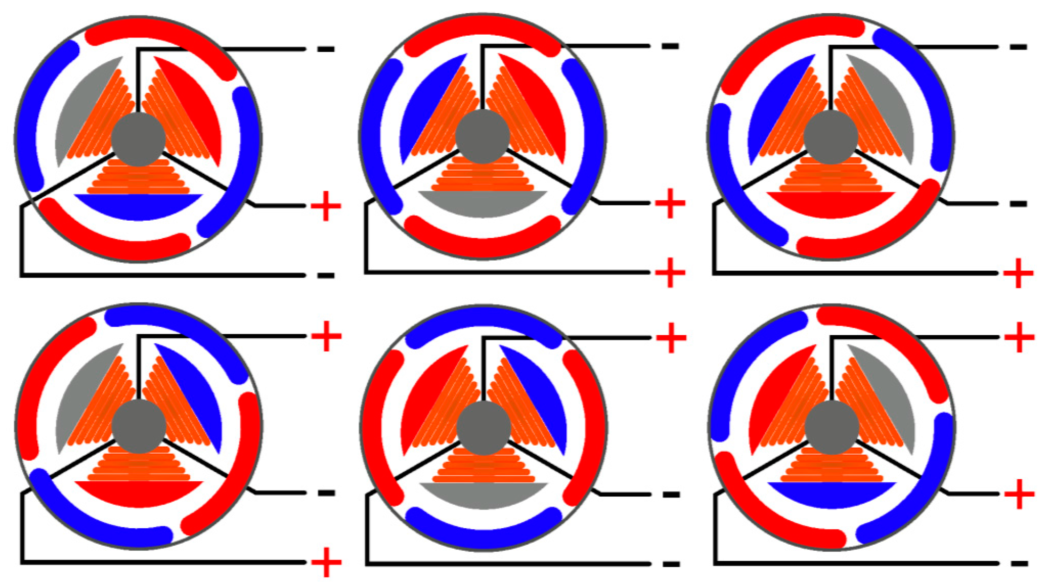
In this section, the general description of a brushless DC motor is given, followed by the concept of controlling a brushless DC motor. There are two major parts of a brushless DC motor, namely the rotor and the stator, as shown in Figure 1. The inner part is named as the stator and outer circular part is called the rotor. The rotor has permanent magnets and the stator consists of three electromagnets. These electromagnets have different polarity due to alternating current. That is why it is called the three-phase rotor. Usually, there is a 120-phase difference between the three electromagnets. Figure 1 shows the phenomenon of rotation of the rotor in a clockwise direction, whereas the polarity of the electromagnets keeps changing. In order to turn the rotor with a constant speed, the polarities are changed at a constant frequency.
A careful look shows that a single electrical rotation causes a half-mechanical rotation . It is determined based on the number of poles, as specified in the following Equation (1).
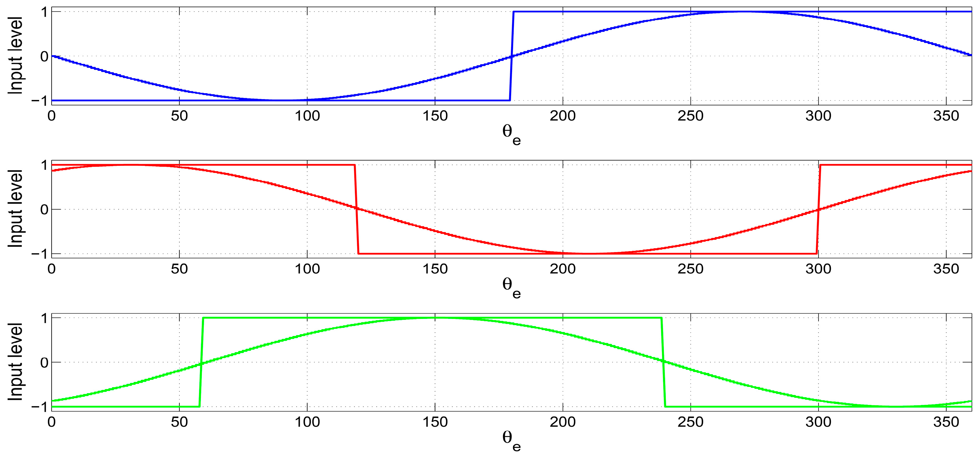
The motor under consideration consists of 14 poles. Hence, one electrical rotation is equal to one seventh of a mechanical rotation. In Figure 2, only low and high signals are shown, which means that each electrical rotation consists of six steps. By using Pulse Width Modulation (PWM) signals, the number of steps can be increased. A PWM signal value varies from 0 to 255. Using these signal values, voltage can be sent from zero percent to hundred percent as depicted in the Figure 2.
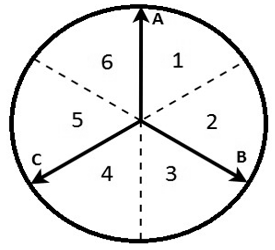
These basic concepts of a BLDC motor help to understand the control structure. The alternating electromagnets producing a rotating space vector. This vector is calculated by following the method proposed as follows. This method reduces the computational time. Figure 3 shows that one electrical rotation is equal to six parts, where A, B, and C are voltage vectors. If both B and C are zero, and voltage A has a value of 255, the resultant vector points in the direction of A. In order to operate in an area, the maximum PWM value is assigned to voltage A, while C is turned off and B can be varied. Table 1 shows the phases used to operate in a particular area. This method shows that every electrical rotation is divided into six parts, and every part can be further divided into 255 steps. Therefore, every electrical rotation consists of 1524 steps (eliminating double scenarios). Hence, a mechanical rotation consists of approximately 10.660 steps. Each step covers nearly 0.03 mechanical degrees.
Table 1 shows the PWM values used to determine the area of the vector in Figure 3, where X means “to be calculated”. With the knowledge of the operating area, the exact value of PWM can be calculated for a certain resultant vector. Note that for each operating area in Equations (2)–(7), the PWM value in the second part of the equation is at its maximum value of 255, but this is left out to make the equations universal.
For Area 1:
For Area 2:
For Area 3:
For Area 4:
For Area 5:
For Area 6:
In Equations (2)–(7), the electrical angle can easily be replaced by the mechanical angle by using formula .
The description of the general theory of a brushless DC motor is now covered and can be used to model the actuator. Moreover, the equations will be used for the mathematical modeling process and position control of the brushless DC motor.
The PWM converter is implemented using Equations (2)–(7) in a MATLAB function. The right equation is selected by using if else statements in MATLAB Programming, and the corresponding PWM values are determined. The input of the function is the controlled angle of the BLDC Motor, and the output is a vector containing the PWM values and the phase corresponding to these values. In Figure 4, the PWM converter subsystem is shown.
The model of the DC motor is a bit more complicated, as can be seen in Figure 5. The PWM converter generates PWM signals for the motor to control the voltage provided to the BLDC motor. The PWM-based control of the voltage is done using the Controlled Voltage Source block in Simulink, with source type DC and initial amplitude zero volts. The input is the PWM value of the PWM converter, the minus side is connected to the ground, and the plus side is the output voltage, which is connected to the DC motor. In this research work, a Permanent Magnet Synchronous Machine (PMSM) is used as DC motor in Simulink. The configuration of the PMSM is standard with three phases, a trapezoidal back Electromotive Force (EMF) waveform, and speed as mechanical input. Since no parameters of the DC motor are known, the parameters of the PMSM are also standard and thus remain unchanged. In Figure 5, N and S shows the North (N) and South (S) pole respectively.
2.2. Experimental and Simulation Data Comparison
To control the motor, an Arduino Nano V3.0, a PWM shield, a PWM driver, motor drivers, capacitors, and MOSFETs are used. In addition, H-bridges are required to control the voltage to the motor and to make sure the back-EMF does not destroy the Arduino or PWM shield. Coding on the Arduino is done in C++. To implement all the devices compactly, a Printed Circuit Board (PCB) is designed and experimental data is used to compare the experimental and simulation results. The simulations are performed in MATLAB using Math works in MATLAB 2014b installed on a Dell precision m3800. In this section, only a basic experimental and simulation test is performed to check if the output of the simulation model corresponds to the measured output. However, this article only discusses the simulation results.
During open-loop operation, the system is operating as expected. Putting a ramp as input resulted in the movement of the motor as would be expected. In Figure 6, the open-loop measurement of a decreasing ramp as input is shown. This shows that the system is working as desired, and the closed-loop algorithm can be implemented.
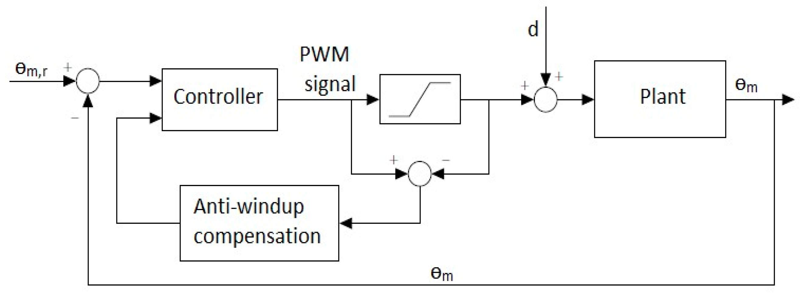
After implementing the closed-loop control algorithm, without a controller, on the Arduino and testing it on a single motor, severe unstable behavior is seen. Therefore, a PID controller, which is commonly used in the industry, is proposed [18]. The control scheme for a BLDC motor can be seen in Figure 7. In this scheme, is the desired mechanical angle, while is the actual measured angle. Since a PID controller is used, anti-windup compensation ensures no integral windup will occur. Note that, normally, cascade control is used to control the position of a PMSM.
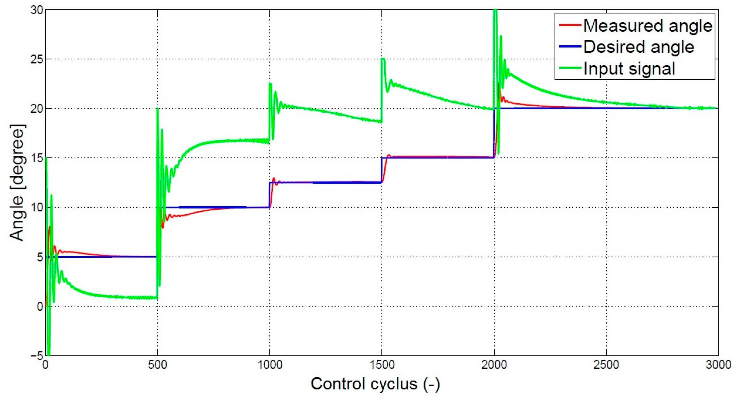
A controller is manually tuned to test the control algorithm and is then implemented on the motor with the same controller values. The closed-loop step responses for the motor are shown in Figure 8. The PID controller has the values of 0.15, 9, and 0.0025 for the P, I, and D, respectively. As can be seen, the step trajectory is roughly followed by the system.
After manual tuning, the Ziegler–Nichols closed-loop tuning method is adopted instead of a trial-and-error method. The Integral and Derivative are neglected in this method, and it is used only as a gain of control. After implementing the PID controllers, a step response for the BLDC motor is shown in Figure 9. As can be seen in the Figure 9, the angle is still vibrating with huge overshoot. In the next section, the simulation and experimental results of both the open-loop and closed-loop are compared.
2.3. Open- and Closed-Loop Measurement and Simulation
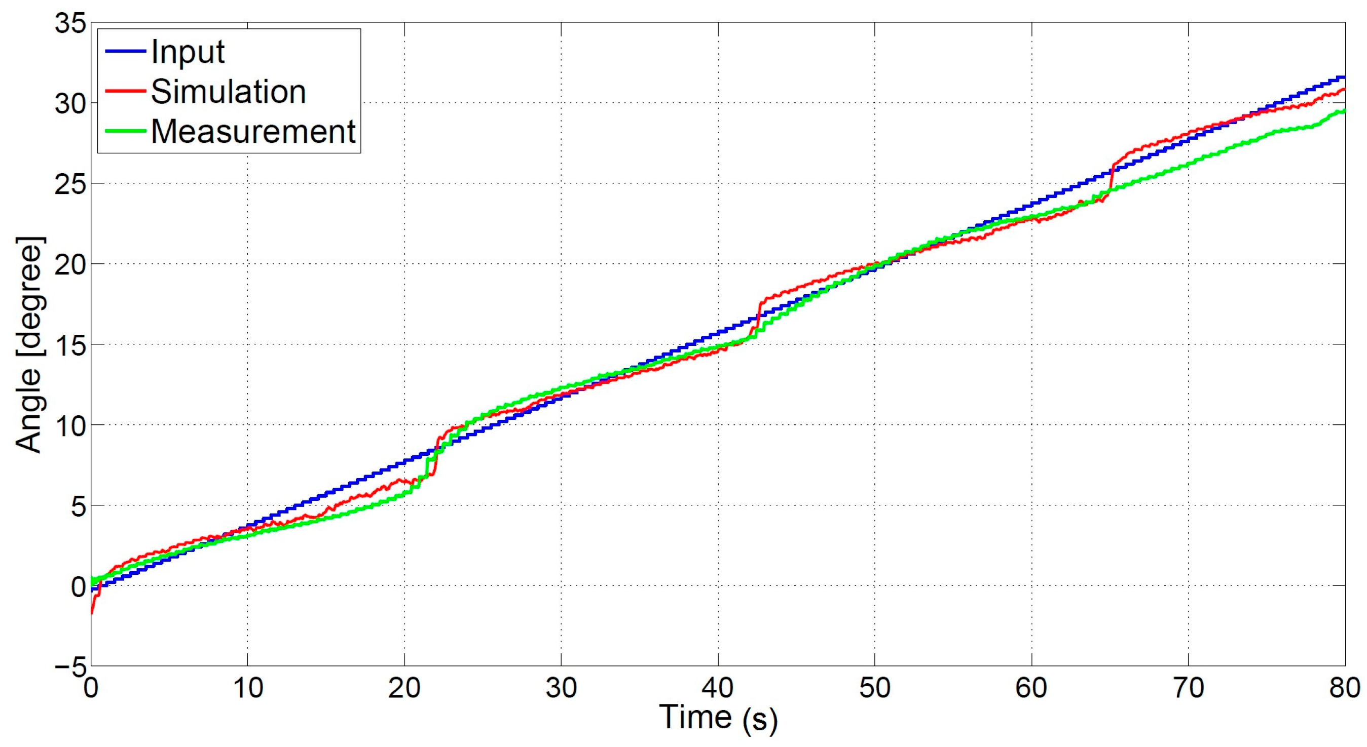
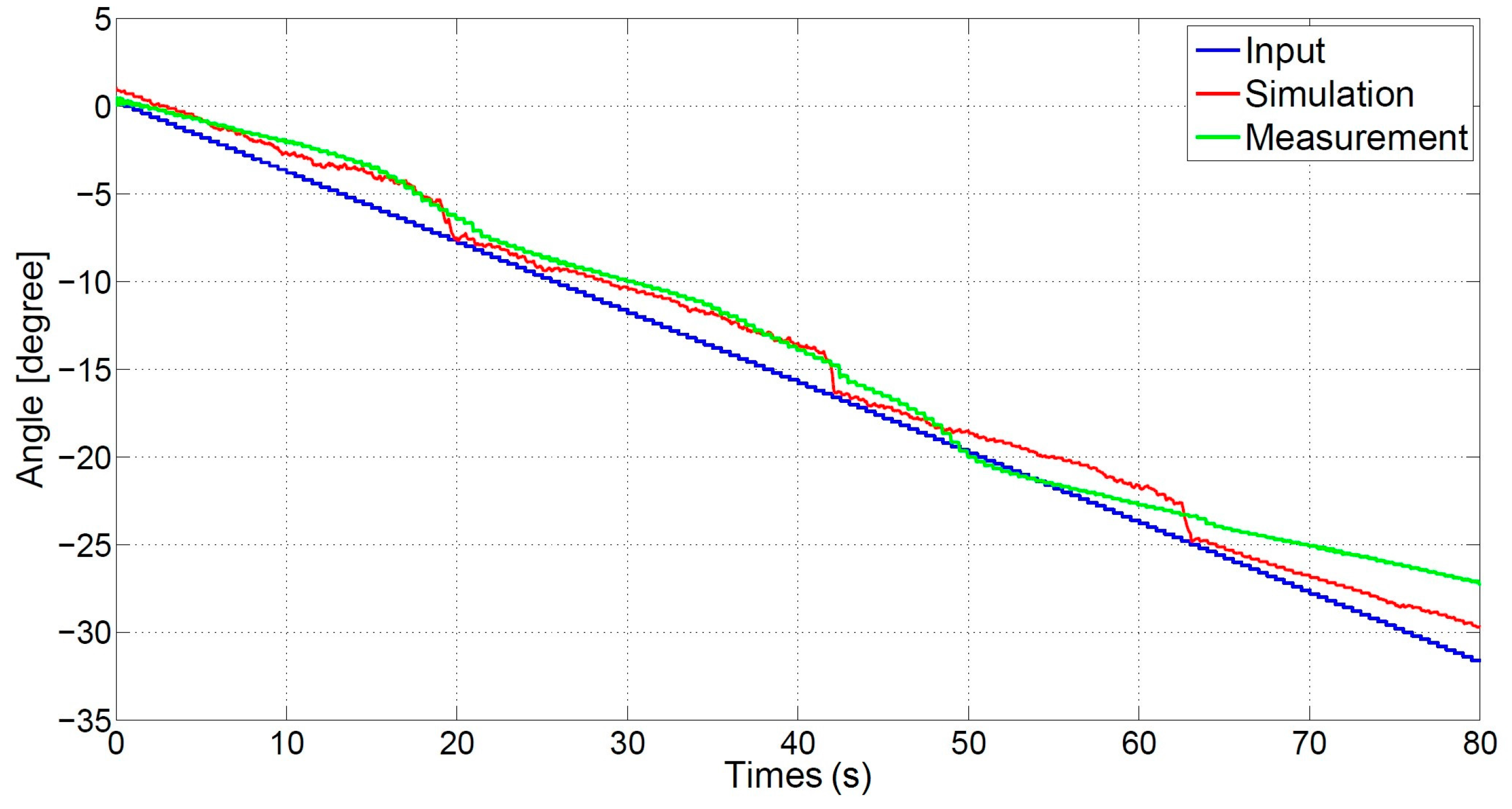
A simple open-loop comparison is completed to check if the output of the simulation model corresponds to the measured output. Both the model and measurement are shown together with the actual and desired measurements in Figure 10 and Figure 11. The two figures are made because differences can occur in moving in the positive and negative directions. It can be seen that the simulation approximates the real measurement, especially at smaller angles. At larger angles, the measurement and simulation data start to differ, especially when looking at the negative direction plot.
Both Figure 10 and Figure 11 indicate that no large discrepancies are present between the model and the measurements. The closed-loop measurements and simulations can now be compared.
The closed-loop measurements and simulations are compared using the same PID controller. The values of the PID controller are determined by using the Ziegler–Nichols method, and are respectively 0.2647, 1.7647, and 0.0099. Figure 12 shows the simulation and measurement data. As seen with the open-loop simulation, for small angles the simulation and measurement data are approximately the same. For larger angles, the simulation and measurement data differ more.
3. DDC Control System Design
3.1. Design of MFAC
Consider the Discrete time nonlinear system having Single Input and Single Output (SISO);
where are the input and output, respectively, at time instant , and is the unknown order, and is an unknown time-varying nonlinear function. Detailed information on the succeeding assumptions is given in reference [19].
Assumption 1:
The proposed system model is observable and controllable, and a bounded control input signal should exist that converts the system response identically to the expected output for the expected bounded system output signal .
Assumption 2:
is a Partial derivative and is continuous with respect to the control input .
Assumption 3:
The general Lipschitz condition should be satisfied by the proposed system.
where , and positive constant .
Nonlinearity is present in the system, which restricts the rate of change of the system.
The purpose of control is to design an appropriate control input to make the system output . is introduced into the criterion function where the system is to linearize in an acceptable range.
The CFDL data model of the control system is described as
The system should satisfy the Assumptions 1–3 for the CFDL method. First, the system is a continuous moving system whose dynamics satisfy the smoothness condition. Second, a bounded change of system input must cause a bounded change of the system when the control input is not out of the permitted range, namely, that the generalized Lipschitz condition is satisfied.
The generalized PPD estimation and MFAC control law can be written as,
where are the step-size constants, is a positive small number, and are weighting factors, and and are the initial values.
The sampling instant values are too small now considering that is a time-varying parameter and can be ignored by . The adaptive based controller is proposed by the integration of Equations (10), (12) and (13). By combining these equations, it will make the Equation (14).
The parameter estimation error is written as . The PPD of the proposed system is , and it is not used in practice. So, by applying rather than the actual value of , the system’s past value is and the parameter estimations are as follows:
Moreover, Equation (14) becomes as follows:
λ is a vital regulating parameter for the MFAC method. The numerical simulation and theoretical analysis confirms that the suitable value of λ will guarantee the stability of the proposed system. The small value of the weighting factor means a lower rise time. More features regarding this parameter are shown in [19,20], respectively.
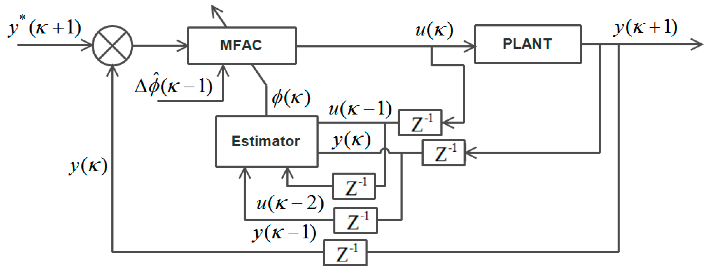
The simulated results show that the appropriate value of that can enhance the general performance of the control system. The main block diagram of MFC is present in Figure 13.
By selecting appropriate parameter, the following result is obtained using the MFAC scheme.
Figure 14 shows the response of the BLDC motor using MFAC. It can be seen that the result is better than the traditional PID method. The overshoot value and settling time is reduced but still needs improvement.
3.2. Design of MFLAC Response
Consider the general discrete time single input, single output (SISO) nonlinear system in Equation (8). The system should satisfy the assumptions in Section 3.1 for the CFDL method.
The basic theory of and stability criteria for MFLAC are present in reference [21]. By using the CFDL scheme, the control algorithm for MFLAC based on a weighted one-step control input criterion function is as follows:
where the weighting function is , and is the criterion function. The introduction of will overcome the deficiencies of the controller.
The general MFAC control law is obtained as follows:
The present approaches for PPD estimation introduce a new parameter estimation criterion as follows:
In Equation (18), the parameter is used to adjust the rate of change of the parameter estimation. From Equation (18), we can get the parameter estimation algorithm in Equation (19):
where is a positive weighting constant, is a step size constant series, , is the initial estimation information of , and is a positive constant.
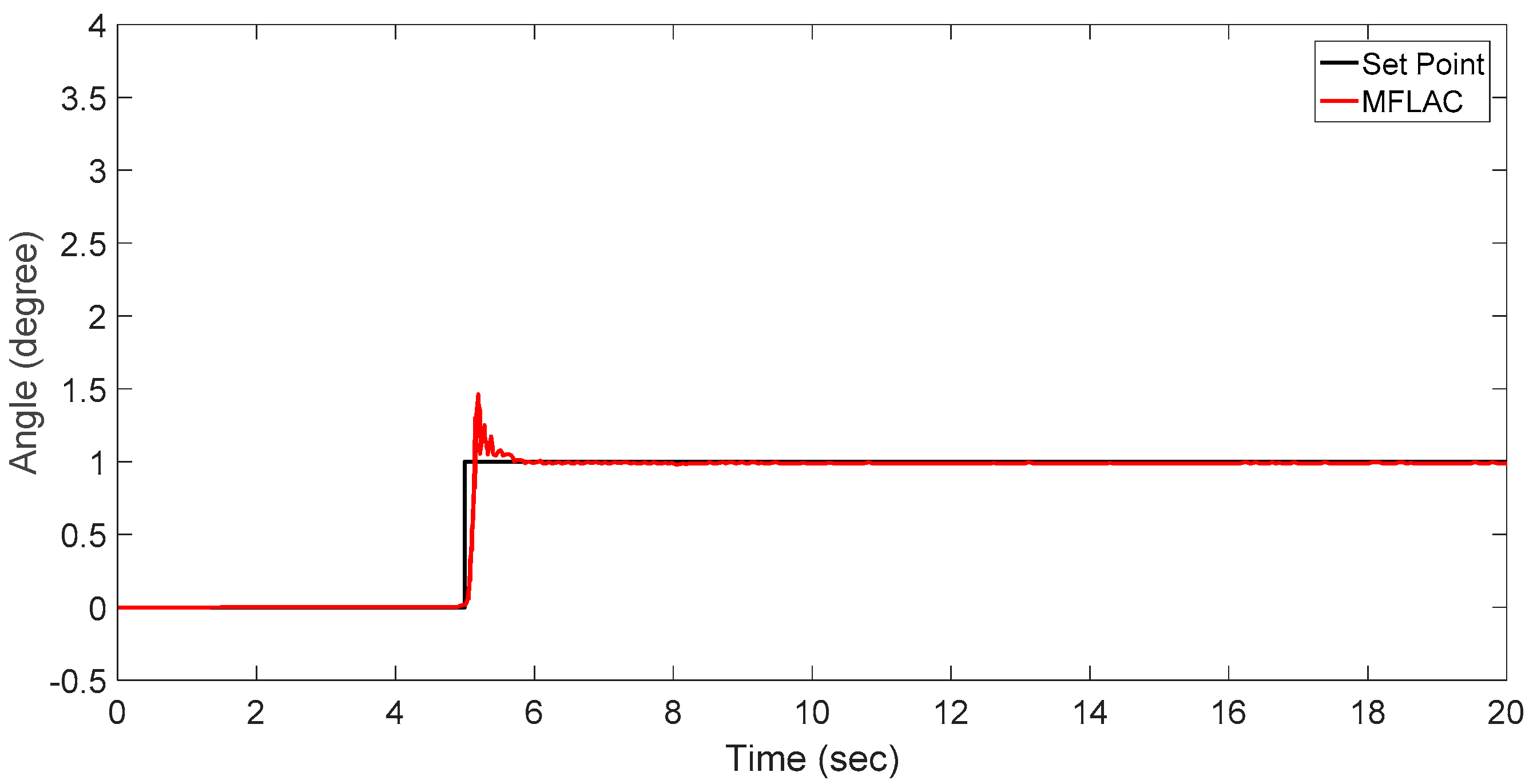
By selecting appropriate parameter, the following result is obtained using the MFLAC scheme.
Figure 15 shows the response of the BLDC Motor using MFLAC. It can be seen that the result is better than the traditional PID and MFAC methods. The overshoot value and settling time is reduced.
3.3. Design of Data-Driven SMC
Consider the general discrete time single input, single output (SISO) nonlinear system in Equation (8). The system should satisfy the assumptions in Section 3.1 for the PFDL method. The basic theory and a stability analysis of MFA-SMC is present in Reference [19].
The discrete sliding mode function is given below:
where c must satisfy the Hurwitz condition . Additionally, the tracking error is , which is well-defined as:
where is the desired tracking trajectory, and is the system output. By using the discrete exponential reaching law,
From Equations (21) and (23), the equivalent derived equation is:
Let
By using Equation (24), the tracking error becomes
Solving Equations (15) and (25) produces the following result:
Combining . Put the value of , and then Equations (21) and (26) establish the following control law:
where .
Since is linear convergence, a slow varying parameter may not be able to satisfy the necessity of the controlled system; therefore, Equation (27) can be improved in the following expression:
where
Equation (27) is the MFA-based SMC control law that converges exponentially and will result in a reduction of time and will not cause problems with stability, where is the weighting factor, is the step sequence, and . Solving Equations (21) and (27) results in stable polynomials that range from .
An analysis shows that is quadratic convergence and that the and values are present in the control law; thus, the MFA-based adaptive SMC is greatly improved. It can be seen that Equation (27) has a discontinuous function. This function will establish a high frequency chattering at the sliding mode surface. This high frequency will reduce the performance of the control system, and cannot be applied to an actual control system. To eliminate the high frequency chattering, replace with the function in Equation (27). By replacing the above function, it will convert the discontinuous function of the continuous signal that will result in a reduction of the chattering effect.
The new control algorithm becomes the following equation:
where .
Integrating Equations (12) and (29) will result in the MFA-based SMC control algorithm. It is observed from the above equation that the MFA-SMC controller design uses a PPD value and only uses the input/output information about the system.
By selecting an appropriate parameter, the following result is obtained using the MFAC-SMC scheme.
Figure 16 shows the response of the BLDC motor using MFA-SMC. It can be seen that the MFA-SMC result in Figure 16 is better than the PID and MFAC methods. The overshoot value and settling time is greatly reduced. The advantages of model-based SMC combined with data-driven MFA are useful and have a great impact on performance.
4. Simulation Results and Analysis
This section discusses the performance analysis between the PID, MFAC, MFLAC, and MFA-SMC schemes.
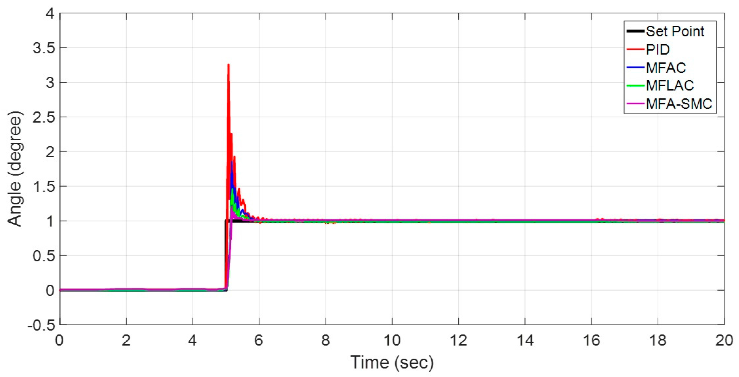
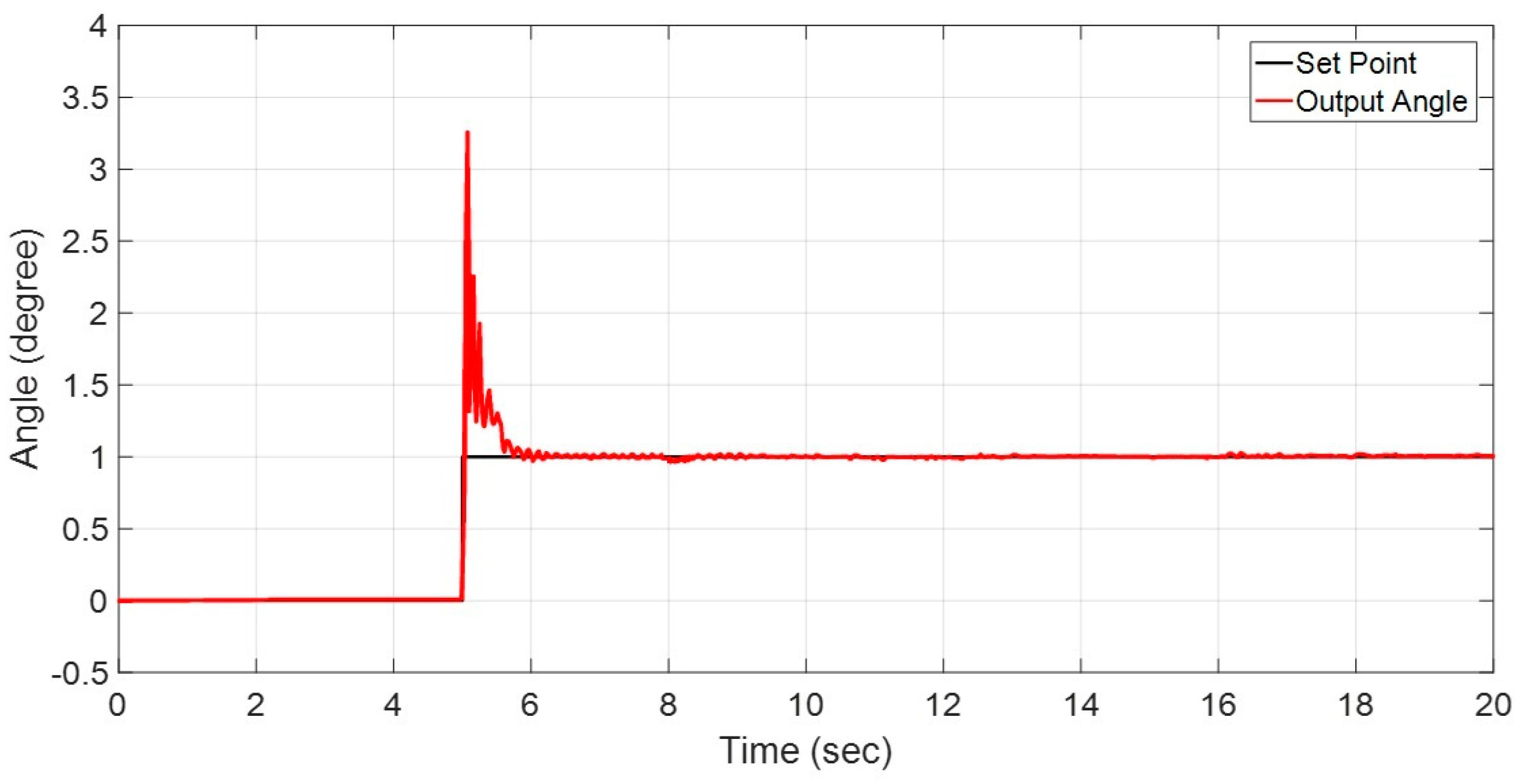
Figure 17 shows the step response of the BLDC motor. Table 2 summarizes the performance analysis of the different control algorithms. Table 2 shows that Conventional PID has a Maximum Overshoot of 3.26, a settling time of 1.251, and a rise time of 0.021. Similarly, MFAC has a Maximum Overshoot of 1.85, a settling time of 0.822, and a rise time of 0.134, and it is better than conventional PID. In addition, MFLAC has a Maximum Overshoot of 1.46, a settling time of 0.691, and a rise time of 0.137. The MFLAC result is much better than PID and MFAC. However, the proposed MFA-based SMC control is greatly improved, with a Maximum Overshoot of 1.21, a settling time of 0.492, and a rise time of 0.146. Although there is only a slight improvement in the rise time, the overshoot and settling time is greatly improved and is better than PID, MFAC, and MFLAC.
SMC has great significance in the theoretical research field. Nowadays, it is becoming a serious source of solutions to industrial problems. Its potential is proscribed simply by the artistic ability of the individuals working in process control. Thus, the expectation for SMC’s application in the processing industries is huge. The primary benefits of SMC are its invariance and quality properties, and that it can deal with bounded modelling uncertainties and bounded disturbances both in linear and nonlinear systems.
Model-Based SMC requires a modelling process, which is expensive and time consuming. To eliminate the modelling process, data-driven SMC is proposed with application to the position control of a three-phase BLDC motor that only depends on the input/output information of the system. The simulation result shows that the overall performance of the three-phase BLDC motor is significantly improved. Moreover, the step response analysis shows that by using MFA-SMC, the maximum overshoot and settling time has greatly reduced, from 3.26 to 1.20 and 1.251 to 0.492, respectively. The proposed MFA-SMC algorithm can achieve better position control and stability over the traditional PID, MFA, and MFLAC methods.
5. Conclusions
In this article, a data–driven MFA-based SMC is used for the position control of a BLDC motor. Moreover, an estimation algorithm and control law are explained for MFA, MFAC, and MFA-SMC algorithms. The proposed control algorithm uses the past-time PPD value, and the necessity of a complex mathematical modeling process is not necessary. The simulation results show that the proposed MFA-based SMC significantly improves position tracking performance and robustness. Moreover, it delivers a concrete theoretical significance by offering a significant enhancement on the basic DDC Algorithm. Moreover, a step response analysis shows that by using MFA-based SMC, the maximum overshoot and settling time has greatly reduced from 3.26 to 1.20 and from 1.251 to 0.492, respectively. A comparative analysis of the simulated results verifies that the proposed MFA-SMC algorithm can achieve better position control and stability over the traditional PID, MFA, and MFLAC methods. The simulation results prove a significant improvement in the performance of the three-phase BLDC motor.
Acknowledgments
This study is supported by the College of Automation Engineering, Nanjing University of Aeronautics and Astronautics Nanjing, China, and is funded by “National Natural Science Foundation of China (NSFC)” under grant No. 61503185. The authors would like to thank the anonymous reviewers for their valuable comments that significantly improved the quality of this paper.
Author Contributions
The central arguments and structure of the paper were equally devised by each of the authors through a series of discussions. Rana Javed Masood conceived the idea and carries out experimental and simulation work under the supervision of Dao bo Wang. Zain Anwar Ali and Babar Khan were involved in the writing of this research article and in the results.
Conflicts of Interest
The author has no conflict of interest.
References
- Krause, P.; Wasynczuk, O.; Sudhoff, S.D.; Pekarek, S. Analysis of Electric Machinery and Drive Systems; John Wiley & Sons: Hoboken, NJ, USA, 2013; Volume 75. [Google Scholar]
- Fitzgerald, A.E.; Kingsley, C.; Umans, S.D. Electric Machinery; McGraw-Hill: New York, NY, USA, 1990. [Google Scholar]
- Matsui, N. Sensorless PM brushless DC motor drives. IEEE Trans. Ind. Electron. 1996, 43, 300–308. [Google Scholar] [CrossRef]
- Matsui, N.; Shigyo, M. Brushless DC motor control without position and speed sensors. IEEE Trans. Ind. Appl. 1992, 28, 120–127. [Google Scholar] [CrossRef]
- Flaig, T.L.; Peterson, G. Controller for a Brushless DC Motor. U.S. Patent 4,528,486, 9 July 1985. [Google Scholar]
- Pillay, P.; Krishnan, R. Modeling, simulation, and analysis of permanent-magnet motor drives. II. The brushless DC motor drive. IEEE Trans. Ind. Appl. 1989, 25, 274–279. [Google Scholar] [CrossRef]
- Trivedi, M.S.; Keshri, R.K. Trajectory based predictive current control for Permanent Magnet Brushless DC motor. In Proceedings of the 2016 IEEE International Conference on Power Electronics, Drives and Energy Systems (PEDES), Trivandrum, India, 14–17 December 2016; pp. 1–6. [Google Scholar]
- Wang, L.; Chai, S.; Yoo, D.; Gan, L.; Ng, K. PID and Predictive Control of Electrical Drives and Power Converters Using MATLAB/Simulink; John Wiley & Sons: Hoboken, NJ, USA, 2015. [Google Scholar]
- Utkin, V. Variable structure systems with sliding modes. IEEE Trans. Autom. Control 1977, 22, 212–222. [Google Scholar] [CrossRef]
- Dursun, E.H.; Durdu, A. Speed Control of a DC Motor with Variable Load Using Sliding Mode Control. Int. J. Comput. Electr. Eng. 2016, 8, 219. [Google Scholar] [CrossRef]
- Rhif, A.; Vaidyanathan, S. Sliding Mode Control Design for a Sensorless Sun Tracker. In Applications of Sliding Mode Control in Science and Engineering; Springer International Publishing: Clam, Switzerland, 2017; pp. 419–434. [Google Scholar]
- Kyslan, K.; Šlapák, V.; Lacko, M.; Ďurovský, F. Cost functions in finite control set model predictive control of permanent magnet DC machine. In Proceedings of the 2015 International Conference on Electrical Drives and Power Electronics (EDPE), Tatranska Lomnica, Slovakia, 21–23 September 2015. [Google Scholar]
- Shahgholian, G.; Maghsoodi, M.; Mahdavian, M.; Janghorbani, M.; Azadeh, M.; Farazpey, S. Analysis of speed control in DC motor drive by using fuzzy control based on model reference adaptive control. In Proceedings of the 2016 13th International Conference on Electrical Engineering/Electronics, Computer, Telecommunications and Information Technology (ECTI-CON), Chiang Mai, Thailand, 28 June–1 July 2016. [Google Scholar]
- Hou, Z.; Jin, S. Data-driven model-free adaptive control for a class of MIMO Nonlinear discrete-time systems. IEEE Trans. Neural Netw. 2011, 22, 2173–2188. [Google Scholar] [PubMed]
- Battistelli, G.; Mosca, E.; Tesi, P. Model-free Adaptive switching control of time-varying plants. IEEE Trans. Autom. Control 2013, 58, 1208–1220. [Google Scholar] [CrossRef]
- Xu, D.; Jiang, B.; Shi, P. A novel model-free adaptive control design for Multivariable industrial processes. IEEE Trans. Ind. Electron. 2014, 61, 6391–6398. [Google Scholar] [CrossRef]
- Zhu, Y.; Hou, Z. Controller dynamic linearization-based model-free adaptive control framework for a class of non-linear system. IET Control Theory Appl. 2015, 9, 1162–1172. [Google Scholar] [CrossRef]
- Cominos, P.; Munro, N. PID controllers: Recent tuning methods and design to specification. IEEE Proc. Control Theory Appl. 2002, 149, 46–53. [Google Scholar] [CrossRef]
- Hou, Z.; Jin, S. Model Free Adaptive Control: Theory and Applications; CRC Press: New York, NY, USA, 2013. [Google Scholar]
- Javed Masood, R.; Wang, D.; Aamir, M.; Ali, Z. MFAC Based SMC Combine Algorithm for the Stability of PMDC. Int. J. Hybrid Inf. Technol. 2017, 10, 15–28. [Google Scholar] [CrossRef]
- Hou, Z.; Huang, W. The model-free learning adaptive control of a class of SISO nonlinear systems. In Proceedings of the American Control Conference, Albuquerque, NM, USA, 6 June 1997; Volume 1, pp. 343–344. [Google Scholar]
Figure 1.
Schematic of the operation of a brushless direct current (DC) motor.

Figure 2.
Visualization of a PWM signal having 255 steps to rotate a DC motor to 360 electrical degrees.
Figure 2.
Visualization of a PWM signal having 255 steps to rotate a DC motor to 360 electrical degrees.

Figure 3.
Schematic of a brushless DC motor.

Figure 4.
The PWM converter subsystem in the Simulink model.
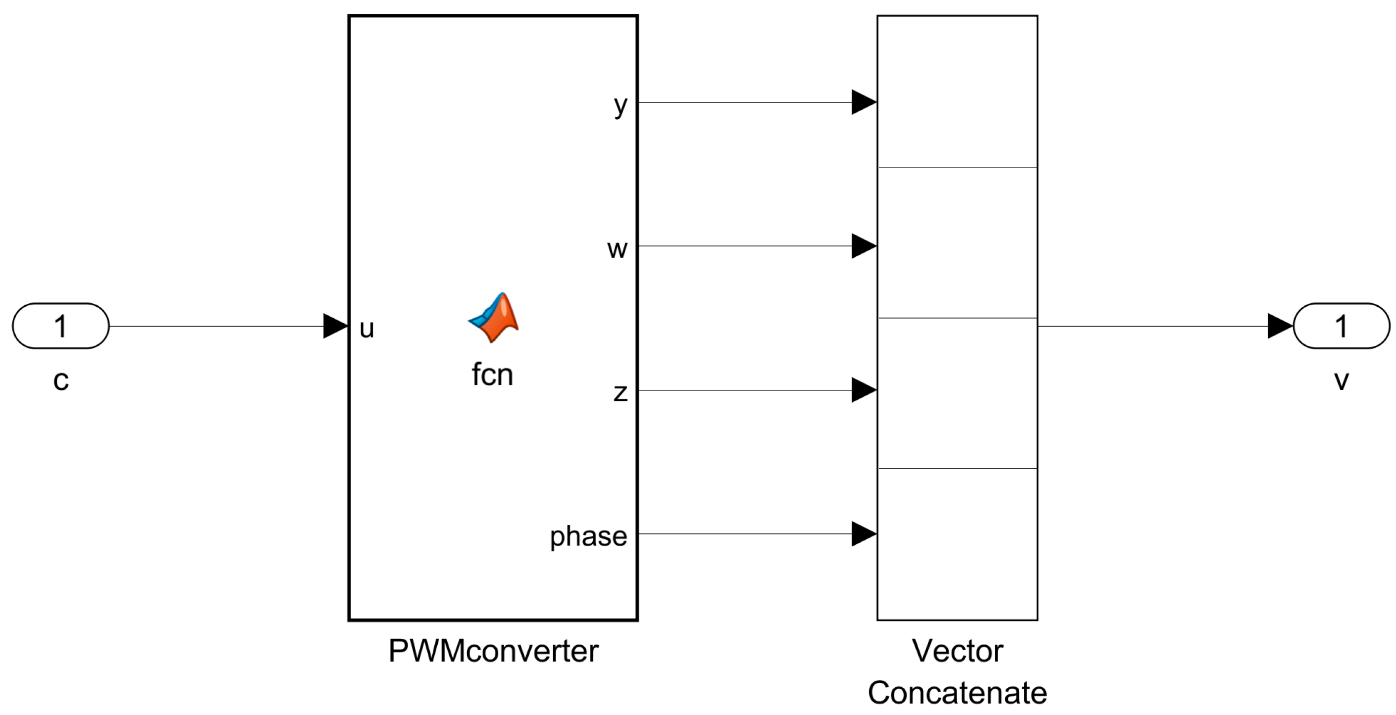
Figure 5.
The DC motor subsystem in the Simulink model.
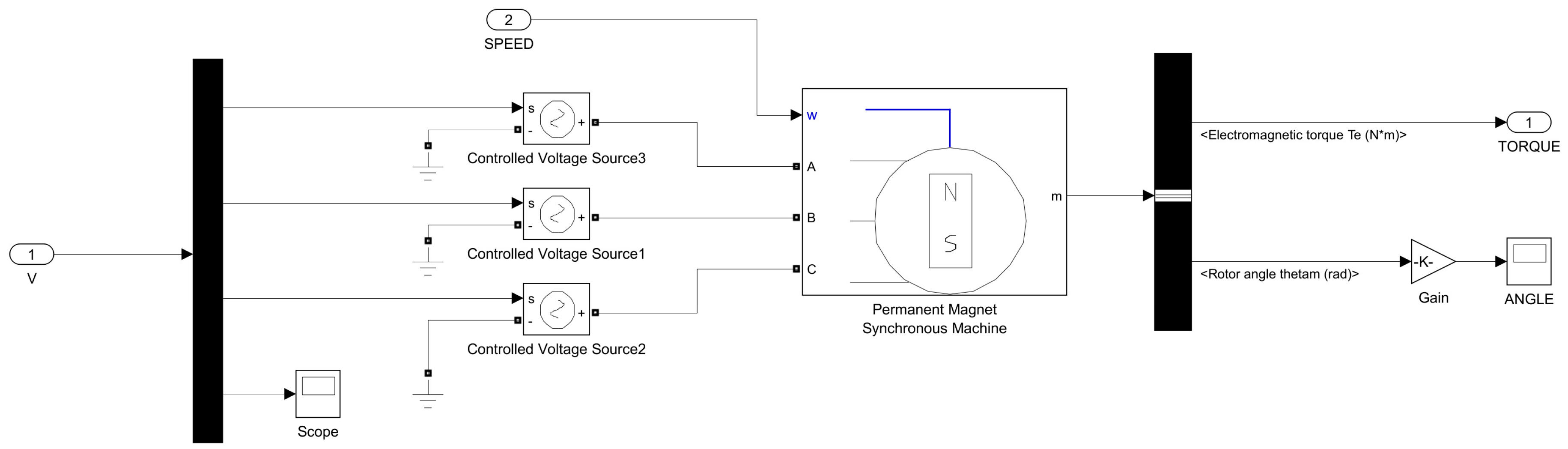
Figure 6.
Open-loop measurement of a decreasing ramp.
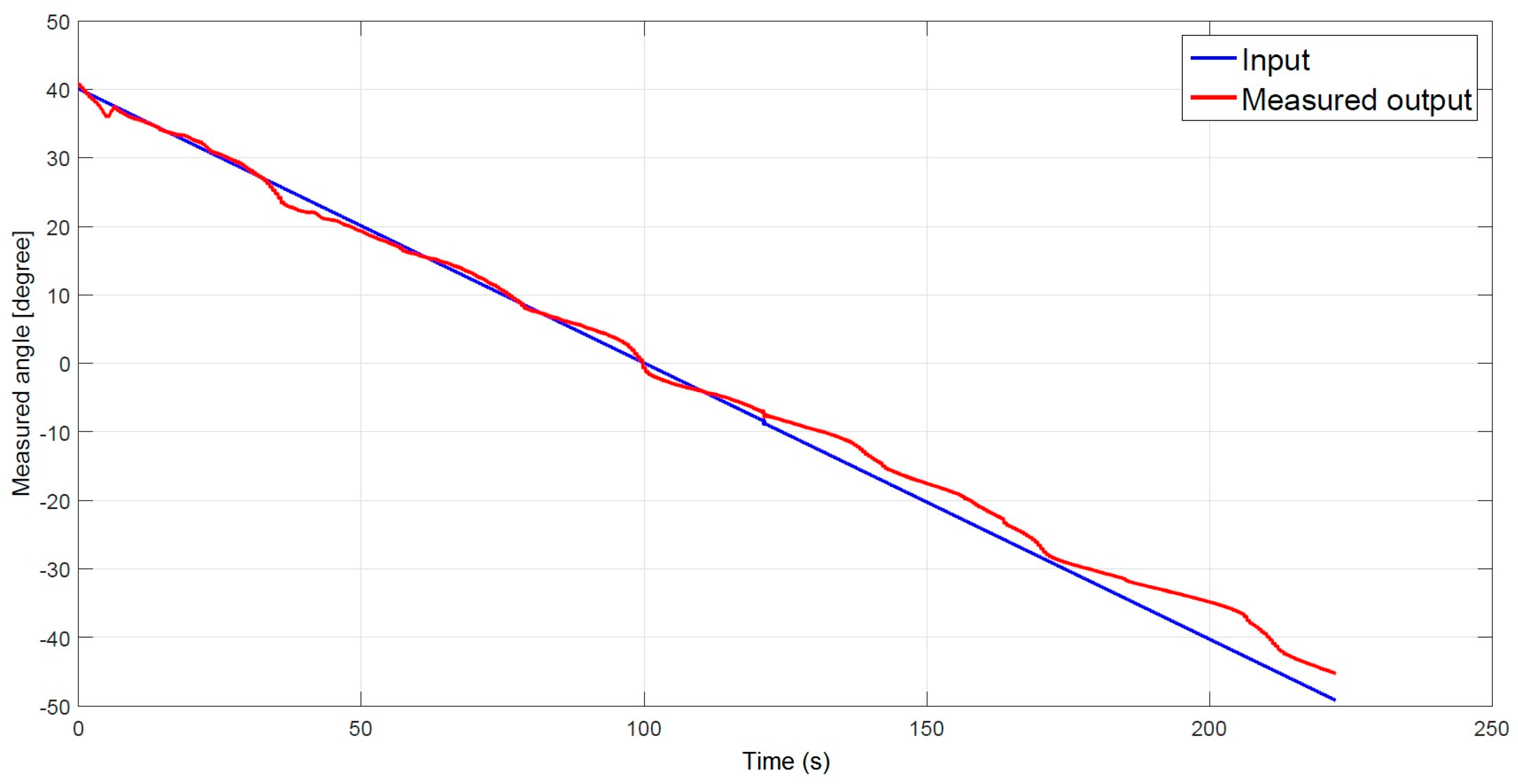
Figure 7.
Control scheme to control a motor.

Figure 8.
Response of the system following a reference trajectory.

Figure 9.
Step response of BLDC Motor using Proportional Integral Derivative.

Figure 10.
Simulation and real measurement in a positive direction.

Figure 11.
Simulation and real measurement in a negative direction.

Figure 12.
Simulation and real measurement of the BLDC motor using steps.
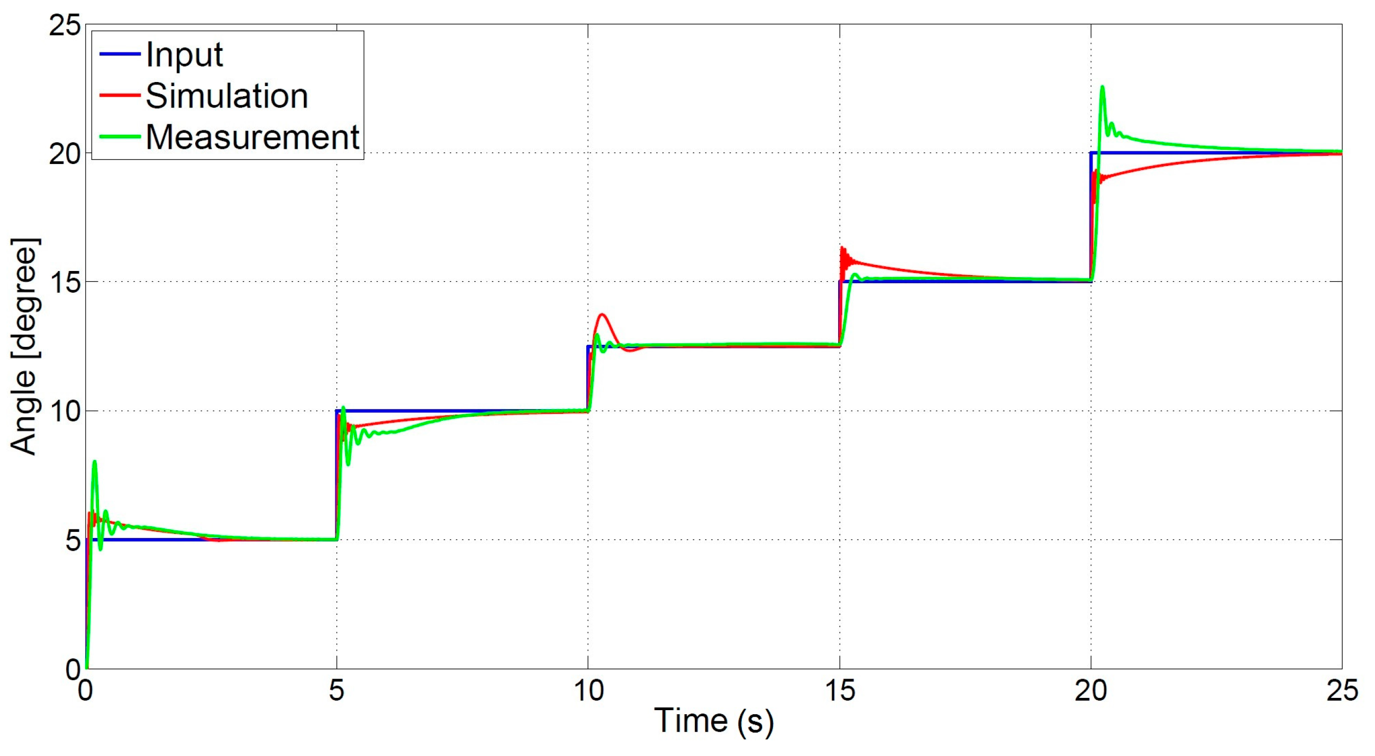
Figure 13.
General Block diagram of Model Free Adaptive Control.

Figure 14.
Step response of BLDC Motor using MFAC.
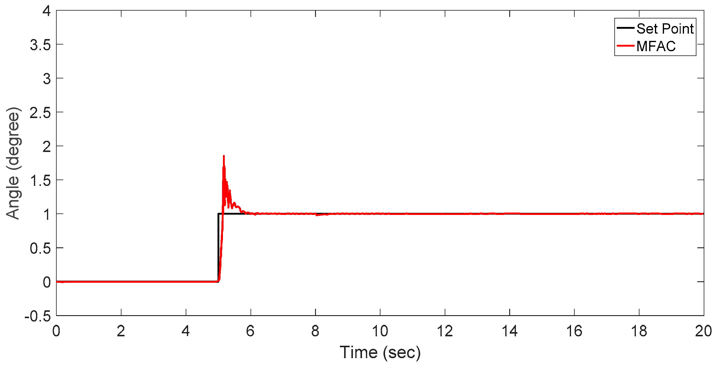
Figure 15.
Step response of the BLDC Motor using MFLAC.

Figure 16.
Step response of BLDC Motor using Model Free Adaptive and Sliding Mode Control.
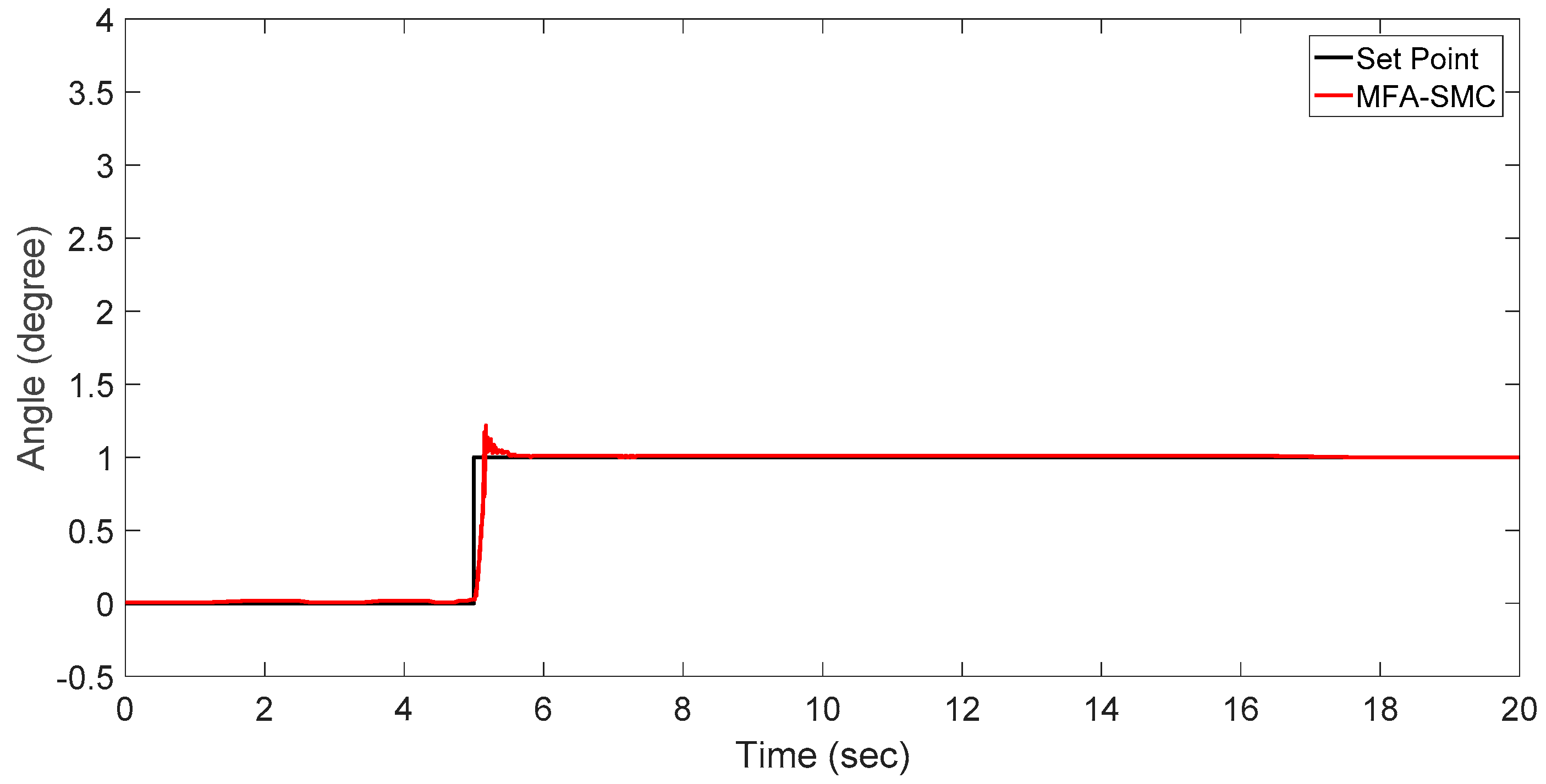
Figure 17.
Comparison analysis of step response of the BLDC motor using PID, MFAC, MFLAC, and MFA-SMC.
Figure 17.
Comparison analysis of step response of the BLDC motor using PID, MFAC, MFLAC, and MFA-SMC.

Table 1.
PWM values to determine the area of the vector in above Figure 3.
Table 1.
PWM values to determine the area of the vector in above Figure 3.
| PWMA (PWM Value) | PWMB (PWM Value) | PWMC (PWM Value) | |
|---|---|---|---|
| Area 1 | 255 | X | 0 |
| Area 2 | X | 255 | 0 |
| Area 3 | 0 | 255 | X |
| Area 4 | 0 | X | 255 |
| Area 5 | X | 0 | 255 |
| Area 6 | 255 | 0 | X |
Table 2.
Comparative analysis of all data-driven control algorithms.
| Algorithm | Maximum Overshoot | Rise Time | Settling Time |
|---|---|---|---|
| PID | 3.26 | 0.021 | 1.251 |
| MFAC | 1.85 | 0.134 | 0.822 |
| MFLAC | 1.46 | 0.137 | 0.691 |
| MFA-SMC | 1.21 | 0.146 | 0.492 |
© 2017 by the authors. Licensee MDPI, Basel, Switzerland. This article is an open access article distributed under the terms and conditions of the Creative Commons Attribution (CC BY) license (http://creativecommons.org/licenses/by/4.0/).
Share and Cite
MDPI and ACS Style
Masood, R.J.; Wang, D.B.; Ali, Z.A.; Khan, B. DDC Control Techniques for Three-Phase BLDC Motor Position Control. Algorithms 2017, 10, 110. https://doi.org/10.3390/a10040110
AMA Style
Masood RJ, Wang DB, Ali ZA, Khan B. DDC Control Techniques for Three-Phase BLDC Motor Position Control. Algorithms. 2017; 10(4):110. https://doi.org/10.3390/a10040110
Chicago/Turabian StyleMasood, Rana Javed, Dao Bo Wang, Zain Anwar Ali, and Babar Khan. 2017. "DDC Control Techniques for Three-Phase BLDC Motor Position Control" Algorithms 10, no. 4: 110. https://doi.org/10.3390/a10040110
Note that from the first issue of 2016, this journal uses article numbers instead of page numbers. See further details here.