Article

Iterative Parameter Estimation Algorithms for Dual-Frequency Signal Models

1
Key Laboratory of Advanced Process Control for Light Industry (Ministry of Education), School of Internet of Things Engineering, Jiangnan University, Wuxi 214122, China
2
School of Internet of Things Technology, Wuxi Vocational Institute of Commerce, Wuxi 214153, China
*
Author to whom correspondence should be addressed.
Algorithms 2017, 10(4), 118; https://doi.org/10.3390/a10040118
Submission received: 15 August 2017 / Revised: 7 October 2017 / Accepted: 11 October 2017 / Published: 14 October 2017

Abstract

:
This paper focuses on the iterative parameter estimation algorithms for dual-frequency signal models that are disturbed by stochastic noise. The key of the work is to overcome the difficulty that the signal model is a highly nonlinear function with respect to frequencies. A gradient-based iterative (GI) algorithm is presented based on the gradient search. In order to improve the estimation accuracy of the GI algorithm, a Newton iterative algorithm and a moving data window gradient-based iterative algorithm are proposed based on the moving data window technique. Comparative simulation results are provided to illustrate the effectiveness of the proposed approaches for estimating the parameters of signal models.

1. Introduction

Parameter estimation is used widely in system identification [1,2,3] and signal processing [4,5]. The existing parameter estimation methods for signal models can be classified into the following basic categories: the frequency-domain methods and the time-domain methods. The frequency-domain methods based on the fast Fourier transform (FFT) mainly include the Rife method, the phase difference method, etc. The accuracy of the Rife method is high in the case of noiseless or higher signal-to-noise ratio with adaptive sampling points; however, the error given by the Rife method is large if the signal frequency is near the DFT quantization frequency point. Therefore, some improved methods were proposed [6,7]. For example, Jacobsen and Kootsookos used three largest spectral lines of the FFT spectrum to calibrate the frequency estimation [8]. Deng et al. proposed a modified Rife method for the frequency shift of signals [9]. However, there is a risk that the shift direction of the frequency may be error. The time-domain methods mainly include the maximum likelihood algorithm, the subspace method and the self-correlation phase method. The maximum likelihood method is effective estimation to minimize the average risk though imposing significant computational costs. The methods in [10,11,12] used multiple autocorrelation coefficients or multi-steps autocorrelation functions to estimate the frequency so the amount of computations increase.
In practice, actual signals are usually disturbed by various stochastic noise, and the time series signals like vibration signals or biomedical signals are subjected to dynamic excitations, including nonlinear and non-stationary properties. In order to solve the difficulties, time-frequency representations (TFR) provide a powerful tool since a TFR can give information about the frequencies contained in signal over time, such as short-time Fourier transform, wavelet transform, and Hilbert–Huang transform [13]. Recently, Amezquita-Sanchez and Adeli presented an adaptive multiple signal classification-empirical wavelet transform methodology for accurate time-frequency representation of noisy non-stationary and nonlinear signals [14]. Daubechies et al. used an empirical mode decomposition-like tool to decompose into the blocks functions, with slowly varying amplitudes and frequencies [15]. These existing approaches can obtain signal models indirectly, because they are realized based on the transform techniques like the Fourier transform and wavelet transform. In this paper, we propose the direct parameter estimation algorithms for signal modeling.
The iterative methods and/or the recursive methods play an important role not only in finding the solutions of nonlinear matrix equations, but also in deriving parameter estimation algorithms for signal models [16,17,18,19,20,21,22]. Furthermore, the iterative algorithms can give more accurate parameter estimates because of making full use of the observed data. Yun utilized the iterative methods to find the roots of nonlinear equations [23]. Dehghan and Hajarian presented an iterative algorithm for solving the generalized coupled Sylvester matrix equations over the generalized centro-symmetric matrices [24]. Wang et al. proposed an iterative method for a class of complex symmetric linear systems [25]. Xu derived a Newton iterative algorithm to the parameter estimation for dynamical systems [26]. Pei et al. used a monotone iterative technique to get the existence of positive solutions and to seek the positive minimal and maximal solutions for a Hadamard type fractional integro-differential equation [27].
As an optimization tool, the Newton method is useful for solving roots of nonlinear problems or deriving parameter estimation algorithms from observed data [28,29,30]. For a long time, the Newton method has been utilized in much literature, such as transcendental equations, minimization and maximization problems, and numerical verification for solutions of nonlinear equations. Simpson noted that the Newton method can be used to give the generalization to systems of two equations and to solve optimization problems [31]. Dennis provided Newton’s method or quasi-Newton methods for multidimensional unconstrained optimization and nonlinear equation problems [32]. Jürgen studied the accelerated convergence of the Newton method by molding a given function into a new one that the roots remain unchanged, but it looks nearly linear in a neighborhood of the root [33]. Djoudi et al. presented a guided recursive Newton method involving inverse iteration to solve the transcendental eigenproblems by reducing it to a generalised linear eigenproblem [34]. Benner described the numerical solution of large-scale Lyapunov equations, Riccati equations, and linear-quadratic optimal control problems [35]. Seinfeld et al. used a quasi-Newton search technique and a barrier modification to enfore closed-loop stability for the H-infinity control problem [36]. Liu et al. presented an iterative identification algorithm for Wiener nonlinear systems using the Newton method [37]. The gradient method with the search directions defined by the gradient of the function at the current point has been developed for optimization problems. For instance, Curry used the gradient descent method for minimizing a nonlinear function of n real variables [38]. Vranhatis et al. studied the development, convergence theory and numerical testing of a class of gradient unconstrained minimization algorithms with adaptive step-size [39]. Hajarian proposed a gradient-based iterative algorithm to find the solutions of the general Sylvester discrete-time periodic matrix equations.
The moving data window with a fixed length is moved as time, which is a first-in-first-out sequence. When a new observation arrives, the data in this moving window are updated by including the new observation and eliminating the oldest one. The length of the moving window remains fixed. The algorithm computes parameter estimates using the observed data in the current window. Recently, Wang et al. presented a moving-window second order blind identification for time-varying transient operational modal parameter identification of linear time-varying structures [41]. Al-Matouq and Vincent developed a multiple-window moving horizon estimation strategy that exploits constraint inactivity to reduce the problem size in long horizon estimation problems [42]. This paper focuses on the parameter estimation problems of dual-frequency signal models. The main contributions of this paper are twofold. The basic idea is to present a gradient-based iterative (GI) algorithm and to estimate the parameters for signal models. Several estimation errors obtained by the Newton iterative and the moving data window based GI algorithms are compared to the errors given by the GI algorithm.
To close this section, we give the outline of this paper. Section 2 derives a GI parameter estimation algorithm. Section 3 and Section 4 propose the Newton and moving data window gradient based iterative parameter estimation algorithms. Section 5 provides an example to verify the effectiveness of the proposed algorithms. Finally, some concluding remarks are given in Section 6.

2. The Gradient-Based Iterative Parameter Estimation Algorithm

Consider the following dual-frequency cosine signal model:
y ( t ) = a cos ( ω 1 t ) + b cos ( ω 2 t ) + v ( t ) ,
where ω 1 > 0 and ω 2 > 0 are the angular frequencies, a > 0 and b > 0 are the amplitudes, t is a continuous-time variable, y ( t ) is the observation, and v ( t ) is a stochastic disturbance with zero mean and variance σ 2 . In actual engineering, we can only get discrete observed data. Suppose that the sampling data are y ( t i ) , i = 1 , 2 , 3 , , L , where L is the data length and t i is the sampling time.
As we all know, signals include the sine signal, cosine signal, Gaussian signal, exponential signal, complex exponential signal, etc. Among them, the sine signal and the cosine signal are typical periodic signals whose waveforms are sine and cosine curves in mathematics. Many periodic signals can be decomposed into the sun of multiple sinusoidal signals with different frequencies and different amplitudes by the Fourier series [43]. The cosine signal differs from the sine signal by π / 2 in the initial phase. This paper takes the double-frequency cosine signal model as an example and derives the parameter estimation algorithms, which are also applicable to the sinusoidal signal models.
Use observed data y ( t i ) and the model output to construct the criterion function
J 1 ( θ ) : = 1 2 i = 1 L [ y ( t i ) a cos ( ω 1 t i ) b cos ( ω 2 t i ) ] 2 .
The criterion function contains the parameters to be estimated, and it represents the error between the observed data and the model output. We hope that this error is as small as possible, which is equivalent to minimizing J 1 ( θ ) and obtaining the estimates of the parameter vector θ : = [ a , b , ω 1 , ω 2 ] T R 4 .
Letting the partial derivative of J 1 ( θ ) with respect to θ be zero gives
grad [ J 1 ( θ ) ] : = J 1 ( θ ) θ = J 1 ( θ ) a , J 1 ( θ ) b , J 1 ( θ ) ω 1 , J 1 ( θ ) ω 2 T R 4 .
Define the stacked output vector Y ( L ) and the stacked information matrix Φ ( θ , L ) as
Y ( L ) : = y ( 1 ) y ( 2 ) y ( L ) R L , Φ ( θ , L ) : = φ T ( θ , 1 ) φ T ( θ , 2 ) φ T ( θ , L ) R L × 4 .
Define the information vector
φ ( θ , t i ) : = [ cos ( ω 1 t i ) , cos ( ω 2 t i ) , a t i sin ( ω 1 t i ) , b t i sin ( ω 2 t i ) ] T R 4 .
Let f ( t i ) : = a cos ( ω 1 t i ) + b cos ( ω 2 t i ) R , and the model output stacked vector
F ( θ , L ) : = f ( θ , 1 ) f ( θ , 2 ) f ( θ , L ) R L .
Then, the gradient vector can be expressed as
grad [ J 1 ( θ ) ] : = Φ T ( θ , L ) [ Y ( L ) F ( θ , L ) ] .
Let k = 1 , 2 , 3 , be an iterative variable and θ ^ k 1 be the estimate of θ at iteration k 1 . The gradient at θ = θ ^ k 1 is given by
grad [ J 1 ( θ ^ k 1 ) ] = J 1 ( θ ^ k 1 ) a , J 1 ( θ ^ k 1 ) b , J 1 ( θ ^ k 1 ) ω 1 , J 1 ( θ ^ k 1 ) ω 2 T R 4 , J 1 ( θ ^ k 1 ) a = i = 1 L cos ( ω ^ 1 , k 1 t i ) [ y ( t i ) a ^ k 1 cos ( ω ^ 1 , k 1 t i ) b ^ k 1 cos ( ω ^ 2 , k 1 t i ) ] , J 1 ( θ ^ k 1 ) b = i = 1 L cos ( ω ^ 2 , k 1 t i ) [ y ( t i ) a ^ k 1 cos ( ω ^ 1 , k 1 t i ) b ^ k 1 cos ( ω ^ 2 , k 1 t i ) ] , J 1 ( θ ^ k 1 ) ω ^ 1 = i = 1 L a ^ k 1 t i sin ( ω ^ 1 , k 1 t i ) [ y ( t i ) a ^ k 1 cos ( ω ^ 1 , k 1 t i ) b ^ k 1 cos ( ω ^ 2 , k 1 t i ) ] , J 1 ( θ ^ k 1 ) ω ^ 2 = i = 1 L b ^ k 1 t i sin ( ω ^ 2 , k 1 t i ) [ y ( t i ) a ^ k 1 cos ( ω ^ 1 , k 1 t i ) b ^ k 1 cos ( ω ^ 2 , k 1 t i ) ] .
Using the negative gradient search and minimizing J 1 ( θ ) , introducing an iterative step-size μ k , we can get the gradient-based iterative (GI) algorithm for dual-frequency signal models:
θ ^ k = θ ^ k 1 μ k grad [ J 1 ( θ ^ k 1 ) ] = θ ^ k 1 μ k Φ T ( θ ^ k 1 , L ) [ Y ( L ) F ( θ ^ k 1 , L ) ] ,
Y ( L ) = [ y ( 1 ) , y ( 2 ) , , y ( L ) ] T ,
Φ ^ k : = Φ ( θ ^ k 1 , L ) = [ φ ( θ ^ k 1 , 1 ) , φ ( θ ^ k 1 , 2 ) , , φ ( θ ^ k 1 , L ) ] T ,
F ^ k : = F ( θ ^ k 1 , L ) = [ f ( θ ^ k 1 , 1 ) , f ( θ ^ k 1 , 2 ) , , f ( θ ^ k 1 , L ) ] T ,
φ ^ k : = φ ( θ ^ k 1 , t i ) = [ cos ( ω ^ 1 , k 1 t i ) , cos ( ω ^ 2 , k 1 t i ) , a ^ k 1 t i sin ( ω ^ 1 , k 1 t i ) , b ^ k 1 t i sin ( ω ^ 2 , k 1 t i ) ] T ,
f ^ k : = f ( θ ^ k 1 , t i ) = a ^ k 1 cos ( ω ^ 1 , k 1 t i ) + b ^ k 1 cos ( ω ^ 2 , k 1 t i ) ,
θ ^ k = [ a ^ k , b ^ k , ω ^ 1 , k , ω ^ 2 , k ] T ,
0 < μ k λ max 1 [ Φ ^ k T Φ ^ k ] .
The steps of the GI algorithm to compute θ ^ k are listed as follows:
  • Let k = 1 , give a small number ε and set the initial value θ ^ 0 = 1 n / p 0 , p 0 is generally taken to be a large positive number, e.g., p 0 = 10 6 .
  • Collect the observed data y ( t i ) , i = 1 , 2 , , L , where L is the data length, form Y ( L ) by Equation (10).
  • Form φ ^ k by Equation (13) and Φ ^ k by Equation (11).
  • Form f ^ k by Equation (14) and F ^ k by Equation (12).
  • Choose a larger μ k satisfying Equation (16), and update the estimate θ ^ k by Equation (15).
  • Compare θ ^ k with θ ^ k 1 , if θ ^ k θ ^ k 1 ε , then terminate this procedure and obtain the iteration time k and the estimate θ ^ k ; otherwise, increase k by 1 and go to Step 3.

3. The Newton Iterative Parameter Estimation Algorithm

The gradient method uses the first derivative, and its convergence rate is slow. The Newton method is discussed here, which requires the second derivative, with fast convergence speed. The following derives the Newton iterative algorithm to estimate the parameters of dual-frequency signal models.
According to the criterion function J 1 ( θ ) in Equation (2). Calculating the second partial derivative of the criterion function J 1 ( θ ) with respect to the parameter θ gives the Hessian matrix
H ( θ ) : = 2 J 1 ( θ ) θ θ T = grad [ J 1 ( θ ) ] θ T .
Let k = 1 , 2 , 3 , be an iterative variable and θ ^ k 1 be the estimate of θ at iteration k 1 . Based on the Newton search, we can derive the Newton iterative (NI) parameter estimation algorithm of dual-frequency signal models:
θ ^ k = θ ^ k 1 H 1 ( θ ^ k 1 ) grad [ J 1 ( θ ^ k 1 ) ] ,
Y ( L ) = [ y ( 1 ) , y ( 2 ) , , y ( L ) ] T ,
Φ ^ k : = Φ ( θ ^ k 1 , L ) = [ φ ( θ ^ k 1 , 1 ) , φ ( θ ^ k 1 , 2 ) , , φ ( θ ^ k 1 , L ) ] T ,
F ^ k : = F ( θ ^ k 1 , L ) = [ f ( θ ^ k 1 , 1 ) , f ( θ ^ k 1 , 2 ) , , f ( θ ^ k 1 , L ) ] T ,
φ ^ k : = φ ( θ ^ k 1 , t i ) = [ cos ( ω ^ 1 , k 1 t i ) , cos ( ω ^ 2 , k 1 t i ) , a ^ k 1 t i sin ( ω ^ 1 , k 1 t i ) , b ^ k 1 t i sin ( ω ^ 2 , k 1 t i ) ] T ,
f ^ k : = f ( θ ^ k 1 , t i ) = a ^ k 1 cos ( ω ^ 1 , k 1 t i ) + b ^ k 1 cos ( ω ^ 2 , k 1 t i ) ,
H ( θ ^ k 1 ) = h 11 ( θ ^ k 1 ) h 12 ( θ ^ k 1 ) h 13 ( θ ^ k 1 ) h 14 ( θ ^ k 1 ) h 21 ( θ ^ k 1 ) h 22 ( θ ^ k 1 ) h 23 ( θ ^ k 1 ) h 24 ( θ ^ k 1 ) h 31 ( θ ^ k 1 ) h 32 ( θ ^ k 1 ) h 33 ( θ ^ k 1 ) h 34 ( θ ^ k 1 ) h 41 ( θ ^ k 1 ) h 42 ( θ ^ k 1 ) h 43 ( θ ^ k 1 ) h 44 ( θ ^ k 1 ) ,
h 11 ( θ ^ k 1 ) = i = 1 L cos 2 ( ω ^ 1 , k 1 t i ) ,
h 12 ( θ ^ k 1 ) = i = 1 L cos ( ω ^ 1 , k 1 t i ) cos ( ω ^ 2 , k 1 t i ) ,
h 13 ( θ ^ k 1 ) = i = 1 L t i sin ( ω ^ 1 , k 1 t i ) [ y ( t i ) b ^ k 1 cos ( ω ^ 2 , k 1 t i ) ] a ^ k 1 t i sin ( 2 ω ^ 1 , k 1 t i ) ,
h 14 ( θ ^ k 1 ) = i = 1 L b ^ k 1 t i cos ( ω ^ 1 , k 1 t i ) sin ( ω ^ 2 , k 1 t i ) ,
h 22 ( θ ^ k 1 ) = i = 1 L cos 2 ( ω ^ 2 , k 1 t i ) ,
h 23 ( θ ^ k 1 ) = i = 1 L a ^ k 1 t i cos ( ω ^ 2 , k 1 t i ) sin ( ω ^ 1 , k 1 t i ) ,
h 24 ( θ ^ k 1 ) = i = 1 L t i sin ( ω ^ 2 , k 1 t i ) [ y ( t i ) a ^ k 1 cos ( ω ^ 1 , k 1 t i ) ] b ^ k 1 t i sin ( 2 ω ^ 2 , k 1 t i ) ] ,
h 33 ( θ ^ k 1 ) = i = 1 L a ^ k 1 t i 2 cos ( ω ^ 1 , k 1 t i ) [ y ( t ) b ^ k 1 cos ( ω ^ 2 , k 1 t i ) ] a ^ k 1 2 t i 2 cos ( 2 ω ^ 1 , k 1 t i ) ,
h 34 ( θ ^ k 1 ) = i = 1 L a ^ k 1 b ^ k 1 t i 2 sin ( ω ^ 1 , k 1 t i ) sin ( ω ^ 2 , k 1 t i ) ,
h 44 ( θ ^ k 1 ) = i = 1 L b ^ k 1 t i 2 cos ( ω ^ 2 , k 1 t i ) [ y ( t ) a ^ k 1 cos ( ω ^ 1 , k 1 t i ) ] b ^ k 1 2 t i 2 cos ( 2 ω ^ 2 , k 1 t i ) .
θ ^ k = [ a ^ k , b ^ k , ω ^ 1 , k , ω ^ 2 , k ] T .
The procedure for computing the parameter estimation vector θ ^ k using the NI algorithm in Equations (18)–(35) is listed as follows:
  • Let k = 1 , give the parameter estimation accuracy ε , set the initial value θ ^ 0 = 1 n / p 0 .
  • Collect the observed data y ( t i ) , i = 1 , 2 , , L , form Y ( L ) by Equation (19).
  • Form φ ^ k by Equation (22), form Φ ^ k by Equation (20).
  • Form f ^ k by Equation (23), form F ^ k by Equation (21).
  • Compute h m n ( θ ^ k 1 ) by Equations (25)–(34), m = 1 , 2 , 3 , 4 , n = 1 , 2 , 3 , 4 , and form H ( θ ^ k 1 ) by Equation (24).
  • Update the estimate θ ^ k by Equation (35).
  • Compare θ ^ k with θ ^ k 1 , if θ ^ k θ ^ k 1 ε , then terminate this procedure and obtain the estimate θ ^ k ; otherwise, increase k by 1 and go to Step 3.

4. The Moving Data Window Gradient-Based Iterative Algorithm

The gradient method and the Newton method use a batch of data, which is the data from t = 1 to t = L . Here, the moving window data from y ( t i p + 1 ) to y ( t i ) , p used here is the length of the moving data window. Let t i be the current sampling time. The moving window data can be represented as y ( t i ) , y ( t i 1 ) ,⋯, y ( t i p + 1 ) . These sampling data change with the sampling time t i . With the increasing of i, the data window moves forward constantly. New data are collected and old data are removed from the window. The following derives the moving data window gradient-based iterative algorithm of dual-frequency signal models.
Define the moving data window criterion function
J 2 ( θ ) : = 1 2 j = 0 p 1 [ y ( t i j ) a cos ( ω 1 t i j ) b cos ( ω 2 t i j ) ] 2 .
Define the information vector
φ ( θ , t i j ) : = [ cos ( ω 1 t i j ) , cos ( ω 2 t i j ) , a t i j sin ( ω 1 t i j ) , b t i j sin ( ω 2 t i j ) ] T R 4 ,
and the stacked information matrix
Φ ( p , θ , t i ) : = [ φ T ( θ , t i ) , φ T ( θ , t i 1 ) , , φ T ( θ , t i p + 1 ) ] T R p × 4 .
Define f ( p , t i j ) : = a cos ( ω 1 t i j ) + b cos ( ω 2 t i j ) R , the vector F ( p , θ , t i ) and Y ( p , t i ) as
F ( p , θ , t i ) : = f ( p , t i ) f ( p , t i 1 ) f ( p , t i P + 1 ) R p , Y ( p , t i ) : = y ( t i ) y ( t i 1 ) y ( t i p + 1 ) R p .
Then, the gradient vector can be expressed as
grad [ J 2 ( θ ) ] : = Φ T ( p , θ , t i ) [ Y ( p , t i ) F ( p , θ , t i ) ] .
Let k = 1 , 2 , 3 , be an iterative variable, and θ ^ k ( t i ) : = [ a ^ k ( t i ) , b ^ k ( t i ) , ω ^ 1 , k ( t i ) , ω ^ 2 , k ( t i ) ] T R 4 be the estimate of θ at iteration k and the sampling time t = t i . Minimizing J 2 ( θ ) and using the negative gradient search, we can obtain the moving data window gradient-based iterative (MDW-GI) algorithm:
θ ^ k ( t i ) = θ ^ k 1 ( t i ) μ k ( t i ) grad [ J 2 ( θ ^ k 1 ( t i ) ) ] = θ ^ k 1 ( t i ) μ k ( t i ) Φ T ( p , θ ^ k 1 ( t i ) , t i ) [ Y ( p , t i ) F ( p , θ ^ k 1 ( t i ) , t i ) ] ,
Φ ^ k ( p , t i ) = Φ ^ k ( p , θ ^ k 1 ( t i ) , t i ) = [ φ ( θ ^ k 1 ( t i ) , t i ) , φ ( θ ^ k 1 ( t i ) , t i 1 ) , , φ ( θ ^ k 1 ( t i ) , t i p + 1 ) ] T ,
Y ( p , t i ) = [ y ( t i ) , y ( t i 1 ) , , y ( t i p + 1 ) ] T ,
F ^ k ( p , t i ) = F ^ k ( p , θ ^ k 1 ( t i ) , t i ) = [ f ( θ ^ k 1 ( t i ) , t i ) , f ( θ ^ k 1 ( t i ) , t i 1 ) , , f ( θ ^ k 1 ( t i ) , t i p + 1 ) ] T ,
φ ^ k ( t i j ) : = φ ( θ ^ k 1 ( t i ) , t i j ) = [ cos ( ω ^ 1 , k 1 ( t i ) t i j ) , cos ( ω ^ 2 , k 1 ( t i ) t i j ) , a ^ k 1 ( t i ) t i j sin ( ω ^ 1 , k 1 ( t i ) t i j ) , b ^ k 1 ( t i ) t i j sin ( ω ^ 2 , k 1 ( t i ) t i j ) ] T ,
f ^ k ( t i j ) : = f ( θ ^ k 1 ( t i ) , t i j ) = a ^ k 1 ( t i ) cos ( ω ^ 1 , k 1 ( t i ) t i j ) + b ^ k 1 ( t i ) cos ( ω ^ 2 , k 1 ( t i ) t i j ) ,
θ ^ k ( t i ) = [ a ^ k ( t i ) , b ^ k ( t i ) , ω ^ 1 , k ( t i ) , ω ^ 2 , k ( t i ) ] T ,
0 < μ k ( t i ) λ max 1 [ Φ ^ k T ( p , t i ) Φ ^ k ( p , t i ) ] .
The steps of the MDW-GI algorithm in Equations (41)–(48) to compute θ ^ k are listed as follows.
  • Pre-set the length of p, let i = p , give the parameter estimation accuracy ε and the iterative length k max = 500 .
  • To initialize, let k = 1 , θ ^ 0 ( t i ) = 1 n / p 0 , p 0 = 10 6 .
  • Collect the observed data y ( t i ) , form Y ( p , t i ) by Equation (43).
  • Form φ ^ k ( t i j ) by Equation (45), form Φ ^ k ( p , t i ) by Equation (42).
  • Form f ^ k ( t i j ) by Equation (46), form F ^ k ( p , t i ) by Equation (44).
  • Select a larger μ k ( t i ) satisfying Equation (48), update the estimate θ ^ k ( t i ) by Equation (47).
  • If k < k max , increase k by 1 and go to Step 4; otherwise, go to the next step.
  • Compare θ ^ k ( t i ) with θ ^ k 1 ( t i ) , if θ ^ k ( t i ) θ ^ k 1 ( t i ) > ε , then let θ ^ 0 ( t i + 1 ) : = θ ^ k ( t i ) , i : = i + 1 , go to Step 2; otherwise, obtain the parameter estimate θ ^ k ( t i ) , terminate this procedure.

5. Examples

Case 1: The numerical simulations of the three iterative algorithms.
Consider the following dual-frequency cosine signal model:
y ( t ) = 1.48 cos ( 0.06 t ) + 2.25 cos ( 0.55 t ) + v ( t ) .
The parameter vector to be estimated is
θ = [ a , b , ω 1 , ω 2 ] T = [ 1.48 , 2.25 , 0.06 , 0.55 ] T .
In simulation, { v ( t ) } is taken as a white noise sequence (stationary stochastic noise) with zero mean and variances σ 2 = 0.50 2 , σ 2 = 1.50 2 and σ 2 = 2.50 2 , respectively. Let t = k T , the sampling period T = 0.005 , k = 2000 , the data length L = 2000 . Apply the proposed GI algorithm using the observed data to estimate the parameters of this signal model. The parameter estimates and their estimation errors δ : = θ ^ k θ / θ × 100 % versus k are as shown in Table 1 and Figure 1.
Apply the NI parameter estimation algorithm in Equations (18)–(35) with the finite observed data to estimate the parameters. The data length and the variances are the same as the condition in the GI algorithm. The parameter estimates and their estimation errors are given in Table 2 and the estimation errors δ versus k are shown in Figure 2.
Apply the MDW-GI parameter estimation algorithm in Equations (41)–(48) to estimate the parameters of signal models. The length p of the moving data window is 100, 200 and 300, and { v ( t ) } is taken as a white noise sequence with zero mean and variance σ 2 = 0.50 2 , respectively. The simulation results are shown in Table 3 and Figure 3.
In order to validate the obtained models, we use the MDW-GI parameter estimates from next-to-last row in Table 3 with p = 300 to construct the MDW-GI estimated model
y ^ ( t ) = 1.46715 cos ( 0.07030 t ) + 2.23197 cos ( 0.55621 t ) .
The estimated outputs y ^ ( t ) and the observed signal model y ( t ) are plotted in Figure 4, where the solid-line denotes the actual signal y ( t ) and the dot-line denotes the estimated signal y ^ ( t ) .
From the simulation results, we can draw the following conclusions:
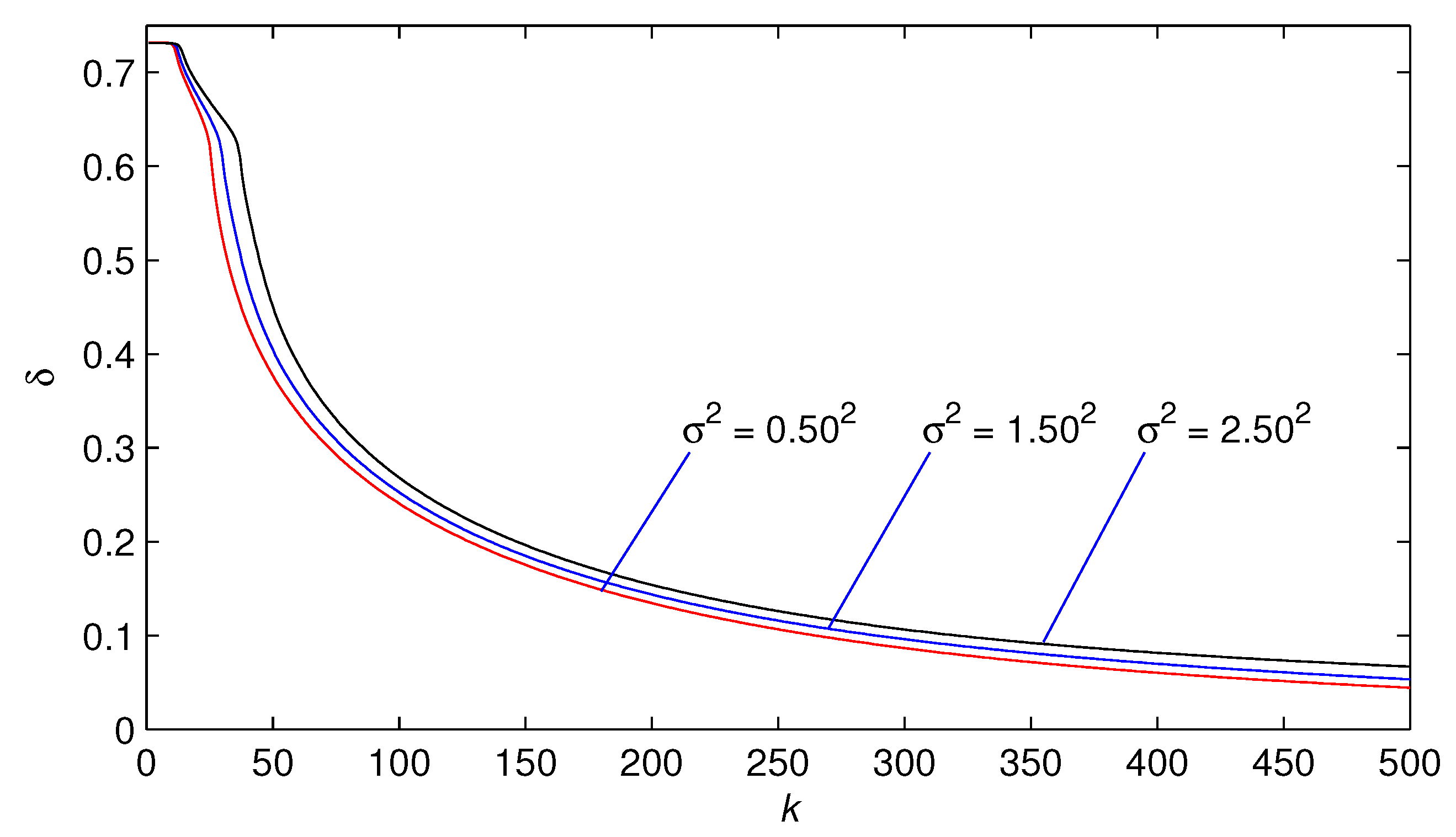
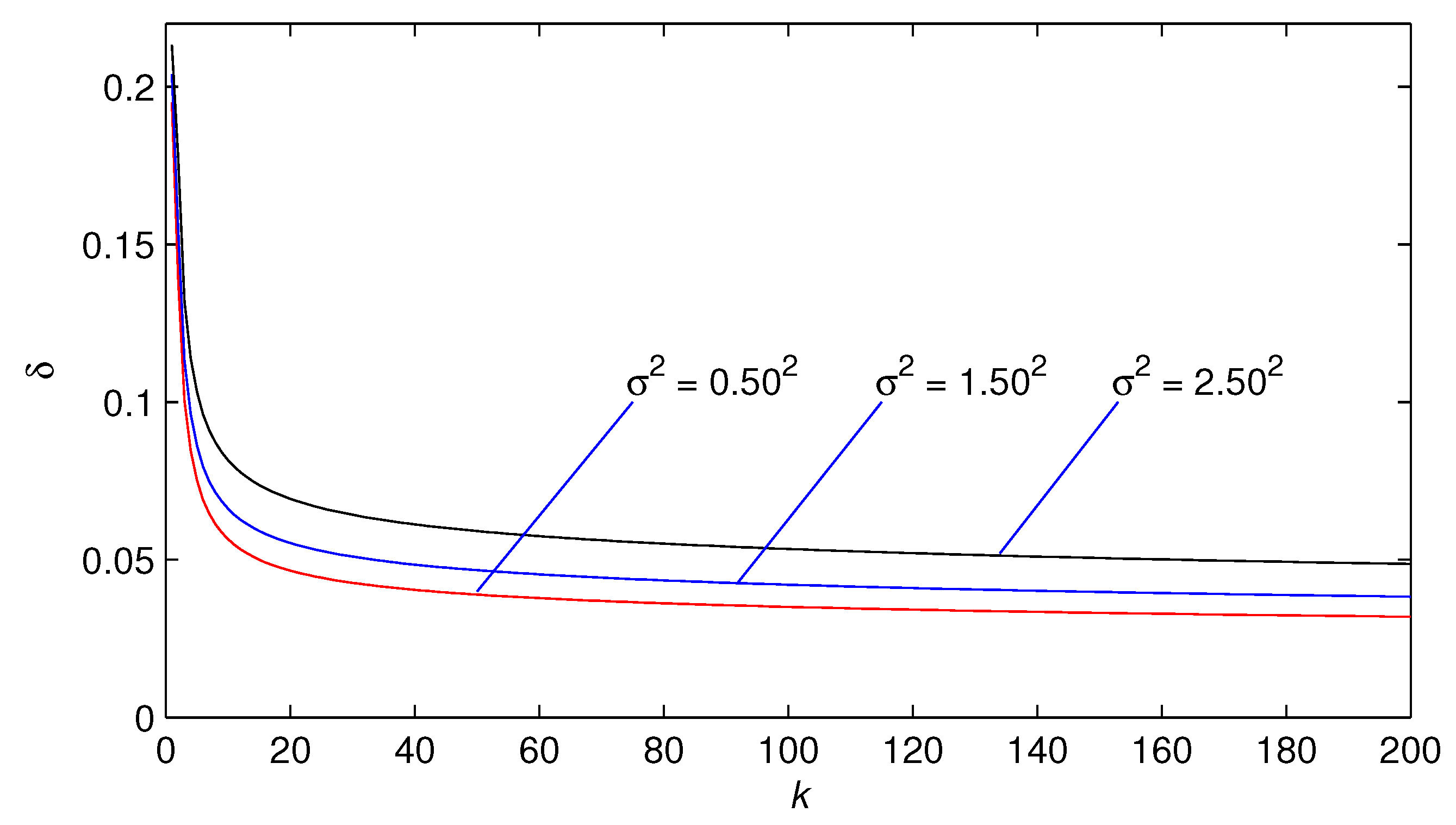
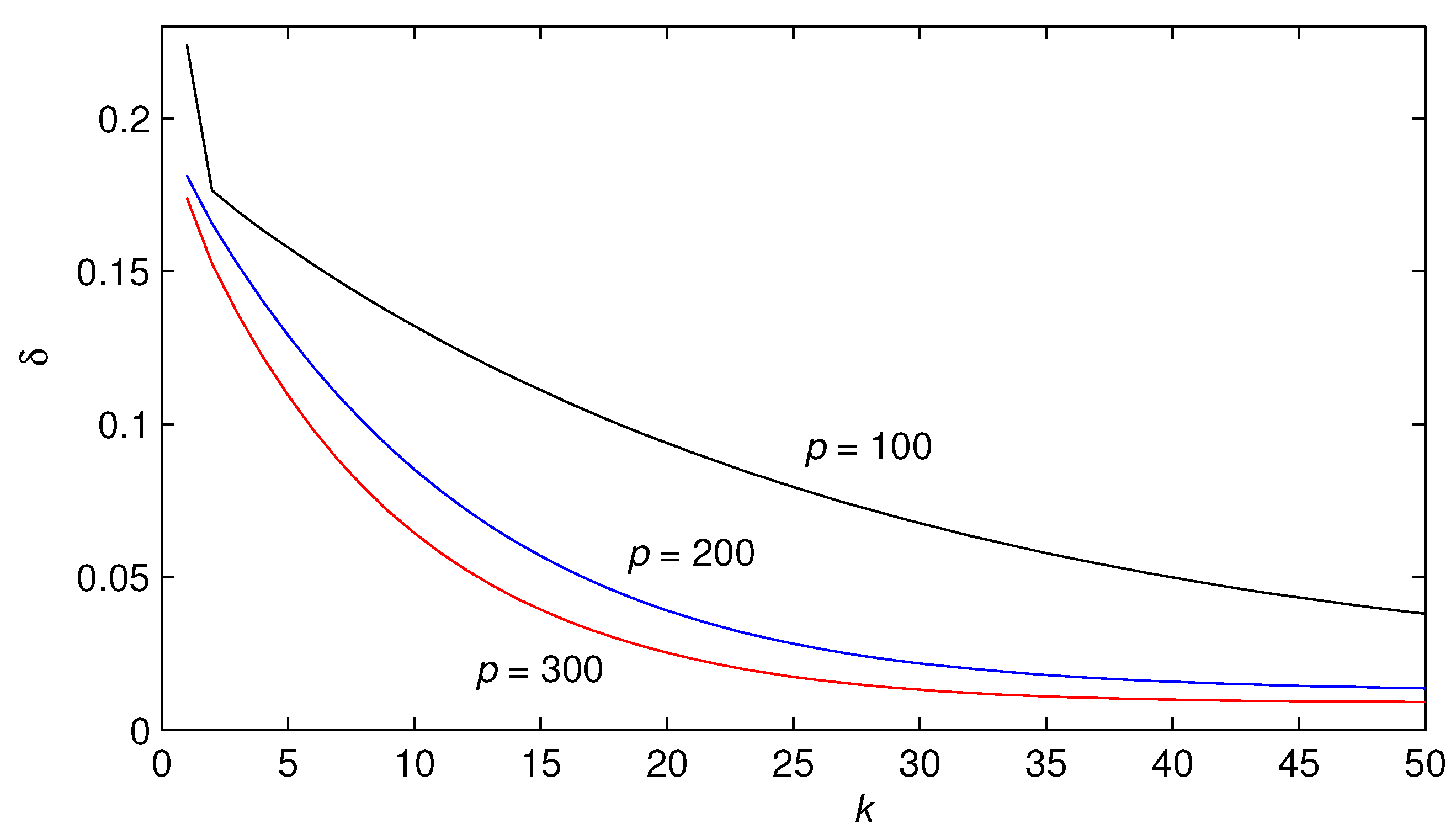
  • The parameter estimation errors obtained by the presented three algorithms gradually decreasing trend as the iterative variable k increases.
  • The parameter estimation errors given by three algorithms become smaller with the noise variance decreasing.
  • Table 1 and Table 2 and Figure 1 and Figure 2 show that the proposed NI algorithm has faster convergence speed and more accurate parameter estimates than the GI algorithm under the same simulation conditions.
  • The larger the length p of the moving data window is, the faster the parameter estimation converge speed is (see Figure 3). Moreover, the larger the length p, the higher the accuracy is (see Table 3).
  • In the simulation, these three algorithms are fulfilled in the same conditions ( σ 2 = 0.50 2 ), and the estimated models obtained by the MDW-GI and NI algorithms have higher accuracy than the GI algorithm.
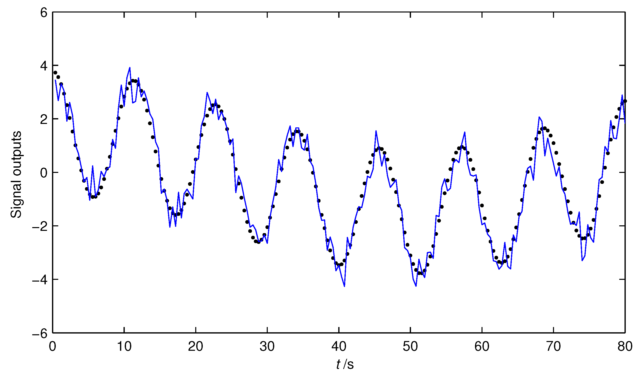
  • The outputs of estimated signal y ^ ( t ) are very close to the actual signal model y ( t ) . In other words, the estimated model can capture the dynamics of the signal.

6. Conclusions

This paper studies the direct parameter estimation algorithms for signal models only using the discrete observed data. By using the gradient search, we need to select a small step-size in order to ensure the convergence, and this will increase the search time and decrease the convergence rate. The proposed NI and MDW-GI algorithms have higher accuracy than the GI estimation algorithm for estimating the unknown parameters. The MWD-GI is used to obtain the parameter estimates at the current moment based on the estimates of previous data obtained at the moment time. Furthermore, the MDW-GI algorithm based on the moving data window technique can estimate the parameters of signal models in real time. The proposed algorithms can be extended to multi-frequency signal models. In the next work, we will consider the estimation of the initial phase of the signal models, that is to say, the signal model is a highly nonlinear function in regard to the frequencies and phases, and estimate all the parameters of dual-frequency signals including the unknown amplitudes, frequencies and initial phases simultaneously.

Acknowledgments

This work was supported by theScience Research of Colleges Universities in Jiangsu Province(No. 16KJB120007, China), and sponsored by Qing Lan Project and the National Natural Science Foundation of China (No. 61492195).

Author Contributions

Feng Ding conceived the idea and supervised his student Siyu Liu to write the paper and Siyu Liu designed and performed the simulation experiments. Ling Xu was involved in the writing of this research article. All authors have read and approved the final manuscript.

Conflicts of Interest

The authors declare no conflict of interest.

References

  1. Ding, F. Complexity, convergence and computational efficiency for system identification algorithms. Control Decis. 2016, 31, 1729–1741. [Google Scholar]
  2. Ding, F.; Wang, F.F. Recursive least squares identification algorithms for linear-in-parameter systems with missing data. Control Decis. 2016, 31, 2261–2266. [Google Scholar]
  3. Xu, L. Moving data window based multi-innovation stochastic gradient identification method for transfer functions. Control Decis. 2017, 32, 1091–1096. [Google Scholar]
  4. Xu, L.; Ding, F. Recursive least squares and multi-innovation stochastic gradient parameter estimation methods for signal modeling. Syst. Signal Process. 2017, 36, 1735–1753. [Google Scholar] [CrossRef]
  5. Xu, L. The parameter estimation algorithms based on the dynamical response measurement data. Adv. Mech. Eng. 2017, 9. [Google Scholar] [CrossRef]
  6. Zhang, Q.G. The Rife frequency estimation algorithm based on real-time FFT. Signal Process. 2009, 25, 1002–1004. [Google Scholar]
  7. Yang, C.; Wei, G. A noniterative frequency estimator with rational combination of three spectrum lines. IEEE Trans. Signal Process. 2011, 59, 5065–5070. [Google Scholar] [CrossRef]
  8. Jacobsen, E.; Kootsookos, P. Fast accurate frequency estimators. IEEE Signal Process. Mag. 2007, 24, 123–125. [Google Scholar] [CrossRef]
  9. Deng, Z.M.; Liu, H.; Wang, Z.Z. Modified Rife algorithm for frequency estimation of sinusoid wave. J. Data Acquis. Process. 2006, 21, 473–477. [Google Scholar]
  10. Elasmi-Ksibi, R.; Besbes, H.; López-Valcarce, R.; Cherif, S. Frequency estimation of real-valued single-tone in colored noise using multiple autocorrelation lags. Signal Process. 2010, 90, 2303–2307. [Google Scholar] [CrossRef]
  11. So, H.C.; Chan, K.W. Reformulation of Pisarenko harmonic decomposition method for single-tone frequency estimation. IEEE Trans. Signal Process. 2004, 52, 1128–1135. [Google Scholar] [CrossRef]
  12. Cao, Y.; Wei, G.; Chen, F.J. An exact analysis of modified covariance frequency estimation algorithm based on correlation of single-tone. Signal Process. 2012, 92, 2785–2790. [Google Scholar] [CrossRef]
  13. Boashash, B.; Khan, N.A.; Ben-Jabeur, T. Time-frequency features for pattern recognition using high-resolution TFDs: A tutorial review. Digit. Signal Process. 2015, 40, 1–30. [Google Scholar] [CrossRef]
  14. Amezquita-Sanchez, J.P.; Adeli, H. A new music-empirical wavelet transform methodology for time-frequency analysis of noisy nonlinear and non-stationary signals. Digit. Signal Process. 2015, 45, 56–68. [Google Scholar] [CrossRef]
  15. Daubechies, I.; Lu, J.F.; Wu, H.T. Synchrosqueezed wavelet transforms: An empirical mode decomposition-like tool. Appl. Comput. Harmon. Anal. 2011, 30, 243–261. [Google Scholar] [CrossRef]
  16. Ding, F.; Xu, L.; Liu, X.M. Signal modeling—Part A: Single-frequency signals. J. Qingdao Univ. Sci. Technol. (Nat. Sci. Ed.) 2017, 38, 1–13. (In Chinese) [Google Scholar]
  17. Ding, F.; Xu, L.; Liu, X.M. Signal modeling—Part B: Dual-frequency signals. J. Qingdao Univ. Sci. Technol. (Nat. Sci. Ed.) 2017, 38, 1–17. (In Chinese) [Google Scholar]
  18. Ding, F.; Xu, L.; Liu, X.M. Signal modeling—Part C: Recursive parameter estimation for multi-frequency signal models. J. Qingdao Univ. Sci. Technol. (Nat. Sci. Ed.) 2017, 38, 1–12. (In Chinese) [Google Scholar]
  19. Ding, F.; Xu, L.; Liu, X.M. Signal modeling—Part D: Iterative parameter estimation for multi-frequency signal models. J. Qingdao Univ. Sci. Technol. (Nat. Sci. Ed.) 2017, 38, 1–11. (In Chinese) [Google Scholar]
  20. Ding, F.; Xu, L.; Liu, X.M. Signal modeling—Part E: Hierarchical parameter estimation for multi-frequency signal models. J. Qingdao Univ. Sci. Technol. (Nat. Sci. Ed.) 2017, 38, 1–15. (In Chinese) [Google Scholar]
  21. Ding, F.; Xu, L.; Liu, X.M. Signal modeling—Part F: Hierarchical iterative parameter estimation for multi-frequency signal models. J. Qingdao Univ. Sci. Technol. (Nat. Sci. Ed.) 2017, 38, 1–12. (In Chinese) [Google Scholar]
  22. Ding, J.L. Data filtering based recursive and iterative least squares algorithms for parameter estimation of multi-input output systems. Algorithms 2016, 9. [Google Scholar] [CrossRef]
  23. Yun, B.I. Iterative methods for solving nonlinear equations with finitely many roots in an interval. J. Comput. Appl. Math. 2013, 236, 3308–3318. [Google Scholar] [CrossRef]
  24. Dehghan, M.; Hajarian, M. Analysis of an iterative algorithm to solve the generalized coupled Sylvester matrix equations. Appl. Math. Model. 2011, 35, 3285–3300. [Google Scholar] [CrossRef]
  25. Wang, T.; Zheng, Q.Q.; Lu, L.Z. A new iteration method for a class of complex symmetric linear systems. J. Comput. Appl. Math. 2017, 325, 188–197. [Google Scholar] [CrossRef]
  26. Xu, L. Application of the Newton iteration algorithm to the parameter estimation for dynamical systems. J. Comput. Appl. Math. 2015, 288, 33–43. [Google Scholar] [CrossRef]
  27. Pei, K.; Wang, G.T.; Sun, Y.Y. Successive iterations and positive extremal solutions for a Hadamard type fractional integro-differential equations on infinite domain. Appl. Math. Comput. 2017, 312, 158–168. [Google Scholar] [CrossRef]
  28. Dehghan, M.; Hajarian, M. Fourth-order variants of Newtons method without second derivatives for solving nonlinear equations. Eng. Comput. 2012, 29, 356–365. [Google Scholar] [CrossRef]
  29. Gutiérrez, J.M. Numerical properties of different root-finding algorithms obtained for approximating continuous Newton’s method. Algorithms 2015, 8, 1210–1216. [Google Scholar] [CrossRef]
  30. Wang, X.F.; Qin, Y.P.; Qian, W.Y.; Zhang, S.; Fan, X.D. A family of Newton type iterative methods for solving nonlinear equations. Algorithms 2015, 8, 786–798. [Google Scholar] [CrossRef]
  31. Simpson, T. The Nature and Laws of Chance; University of Michigan Library: Ann Arbor, MI, USA, 1740. [Google Scholar]
  32. Dennis, J.E.; Schnable, R.B. Numerical Methods for Unconstrained Optimization and Nonlinear Equations; Prentice-Hall: Englewood Cliffs, NJ, USA, 1983. [Google Scholar]
  33. Jürgen, G. Accelerated convergence in Newton’s method. Soc. Ind. Appl. Math. 1994, 36, 272–276. [Google Scholar]
  34. Djoudi, M.S.; Kennedy, D.; Williams, F.W. Exact substructuring in recursive Newton’s method for solving transcendental eigenproblems. J. Sound Vib. 2005, 280, 883–902. [Google Scholar] [CrossRef]
  35. Benner, P.; Li, J.R.; Penzl, T. Numerical solution of large-scale Lyapunov equations, Riccati equations, and linear-quadratic optimal control problems. Numer. Linear Algebra Appl. 2008, 15, 755–777. [Google Scholar] [CrossRef]
  36. Seinfeld, D.R.; Haddad, W.M.; Bernstein, D.S.; Nett, C.N. H2/H controller synthesis: Illustrative numerical results via quasi-newton methods. Numer. Linear Algebra Appl. 2008, 15, 755–777. [Google Scholar]
  37. Liu, M.M.; Xiao, Y.S.; Ding, R.F. Iterative identification algorithm for Wiener nonlinear systems using the Newton method. Appl. Math. Model. 2013, 37, 6584–6591. [Google Scholar] [CrossRef]
  38. Curry, H.B. The method of steepest descent for non-linear minimization problems. Q. Appl. Math. 1944, 2, 258–261. [Google Scholar] [CrossRef]
  39. Vrahatis, M.N.; Androulakis, G.S.; Lambrinos, J.N.; Magoulas, G.D. A class of gradient unconstrained minimization algorithms with adaptive stepsize. J. Comput. Appl. Math. 2000, 114, 367–386. [Google Scholar] [CrossRef]
  40. Hajarian, M. Solving the general Sylvester discrete-time periodic matrix equations via the gradient based iterative method. Appl. Math. Lett. 2016, 52, 87–95. [Google Scholar] [CrossRef]
  41. Wang, C.; Wang, J.Y.; Zhang, T.S. Operational modal analysis for slow linear time-varying structures based on moving window second order blind identification. Signal Process. 2017, 133, 169–186. [Google Scholar] [CrossRef]
  42. Al-Matouq, A.A.; Vincent, T.L. Multiple window moving horizon estimation. Automatica 2015, 53, 264–274. [Google Scholar] [CrossRef]
  43. Boashash, B. Estimating and interpreting the instantaneous frequency of a signal—Part 1: Fundamentals. Proc. IEEE 1992, 80, 520–538. [Google Scholar] [CrossRef]
Figure 1. The GI estimation errors δ versus k.
Algorithms 10 00118 g001
Figure 2. The NI estimation errors δ versus k.
Algorithms 10 00118 g002
Figure 3. The MDW-GI estimation errors δ versus k ( σ 2 = 0.50 2 ).
Algorithms 10 00118 g003
Figure 4. The estimated outputs y ^ ( t ) and the actual signal model y ( t ) versus t. Solid line: the actual output y ( t ) , dot-line: the estimated signal y ^ ( t ) .
Algorithms 10 00118 g004
Table 1. The GI parameter estimates and errors.
σ 2 kab ω 1 ω 2 δ ( % )
2.50 2 100.553500.553500.000640.0014873.11514
200.612110.615280.033250.1476868.89718
501.066941.082760.000000.5811645.10172
1001.200741.569910.000020.5648326.83480
2001.282321.880590.000180.5603015.39800
5001.349252.129400.014730.557676.68183
1.50 2 100.552900.552900.002120.0048773.10844
200.634830.636290.025490.1793167.62638
501.102991.204780.000020.5647840.47663
1001.219211.609040.000140.5581225.26461
2001.299941.903430.001370.5542814.36541
5001.376652.148980.035820.554435.33204
0.50 2 100.552370.552400.006040.0138773.04062
200.659580.656530.016240.2137766.34478
501.094601.289180.000090.5585237.71802
1001.223321.642710.000260.5522824.07888
2001.313231.925380.001580.5486413.44312
5001.390902.174890.024500.547414.43172
True values1.480002.250000.060000.55000
Table 2. The NI parameter estimates and errors.
σ 2 kab ω 1 ω 2 δ ( % )
2.50 2 11.830601.782680.099230.5208721.32333
21.847361.936210.133600.5585217.77782
101.680782.164200.110200.562168.16074
201.656752.196560.105970.561596.93411
1001.620362.230240.097480.558895.34256
2001.608602.237780.094160.557634.86795
1.50 2 11.807861.797280.098830.5238020.40210
21.782331.956540.122410.5556415.49323
101.635632.166560.102870.560226.61985
201.616192.195880.099430.560055.53200
1001.587962.225300.092560.558234.20939
2001.578982.231500.089880.557303.82961
0.50 2 11.785291.811180.098450.5267019.51195
21.734671.970380.115190.5545313.90292
101.603142.163840.098470.559785.65377
201.587032.190390.095700.559914.65522
1001.564612.216170.090230.558713.50636
2001.557662.221290.088120.558033.19386
True values1.480002.250000.060000.55000
Table 3. The MDW-GI parameter estimates and errors ( σ 2 = 0.50 2 ).
pkab ω 1 ω 2 δ ( % )
10011.582541.643390.077850.5775022.40827
21.875941.975970.111250.5790717.64461
51.832272.003690.110200.5780115.77345
101.778872.051360.108790.5760513.20660
201.698922.123390.105260.572209.37923
501.577512.233980.091530.561743.79684
20011.786041.859700.102560.5701118.12068
21.818801.950550.109310.5724316.56384
51.737912.012450.109970.5742012.91251
101.641482.089260.108710.574498.52118
201.539162.171650.099060.569443.90746
501.479382.220550.080730.560511.36478
30011.746061.855860.108810.5697917.40188
21.788541.973090.116160.5730315.23989
51.697042.050380.115280.5745810.94891
101.597052.128400.108770.572516.44220
201.509432.196780.090340.564122.52463
501.467152.231970.070300.556210.91639
True values1.480002.250000.060000.55000

