Improvement of ID3 Algorithm Based on Simplified Information Entropy and Coordination Degree

1
School of Control Science and Engineering, Shandong University, Jinan 250061, China
2
School of Mechanical, Electrical and Information Engineering, Shandong University, Weihai 264209, China
3
Department of Electrical Engineering and Information Technology, Shandong University of Science and Technology, Jinan 250031, China
*
Author to whom correspondence should be addressed.
Algorithms 2017, 10(4), 124; https://doi.org/10.3390/a10040124
Submission received: 2 September 2017
/
Revised: 29 October 2017
/
Accepted: 2 November 2017
/
Published: 6 November 2017
Abstract
:The decision tree algorithm is a core technology in data classification mining, and ID3 (Iterative Dichotomiser 3) algorithm is a famous one, which has achieved good results in the field of classification mining. Nevertheless, there exist some disadvantages of ID3 such as attributes biasing multi-values, high complexity, large scales, etc. In this paper, an improved ID3 algorithm is proposed that combines the simplified information entropy based on different weights with coordination degree in rough set theory. The traditional ID3 algorithm and the proposed one are fairly compared by using three common data samples as well as the decision tree classifiers. It is shown that the proposed algorithm has a better performance in the running time and tree structure, but not in accuracy than the ID3 algorithm, for the first two sample sets, which are small. For the third sample set that is large, the proposed algorithm improves the ID3 algorithm for all of the running time, tree structure and accuracy. The experimental results show that the proposed algorithm is effective and viable.
1. Introduction
Large amount of data that includes a lot of potential and valuable information is stored in a database. If a wealth of hidden information can be extracted from the database, more potential value will be created. Faced with the challenge of the above issue, data mining [1,2] technologies came into being and showed strong vitality. Data mining includes several important technologies such as classification [3], clustering [4], regression [5], etc. The classification mining technology, among data mining technologies, is becoming a most active and mature research direction allowing for successful applications. Classification mining [6] can be applied to discover useful information from large amounts of data stored in a large number of fields such as hospital, stock, banking, etc. For example, it is important for a hospital to accurately predict the length of stay (LOS), and Ref. [7] showed that the classification mining technology was not only beneficial to solve limited bed resources, but was also helpful for the hospital staff to implement better planning and management of hospital resources. In Ref. [8], in order to easily acquire stock returns in the stock market, different classifiers were used in the stock market prediction, and the prediction accuracy was commonly satisfied. Ref. [9] used two types of classifier ensembles to predict stock returns. The problem of bank note recognition is very important for bank staff. Ref. [10] presented neuro-classifiers to address the big problem. Ref. [11] presented the ANN classification approach, which could be used to detect early warning signals of potential failures for banking sectors.
The decision tree methods [12,13], the neural network methods [14] and the statistical methods [15,16] are common classification algorithms used by researchers in the field of classification mining. A large amount of decision tree algorithms such as Iterative Dichotomizer 3 (ID3) [17], C4.5 [18], and Classification And Regression Tree (CART) [19] are used in different fields. Most decision tree methods are developed from the ID3 method. For example, the C4.5 method [20] presented an optimal attribution selection standard (gain ratio) [21] instead of the optimal attribution selection standard (information gain) in ID3; The CART method took the Gini index [22] as the selection standard of the optimal attribution. Although many advantages are acquired from these improved decision tree methods, there is also much room for improvement.
The ID3 algorithm is used as a general classification function, and it has many advantages, such as understandable decision rules and the intuitive model. Nevertheless, ID3 also has some disadvantages, for example: (1) there exists a problem of multi-value bias in the process of attribute selection [23], but the attribution that has more values is not always optimal; (2) it is not easy to calculate information entropy [24,25] by using logarithmic algorithms, which costs a lot of time; and (3) the tree size is difficult to control [26], and the tree with a big size requires many long classification rules.
In order to solve the problems above, an optimized scheme is proposed here based on the ID3 method. First of all, in order to solve the defect of multi-value bias brought by the information gain equation in ID3, C4.5 selected gain ratio instead of the information gain equation, but this method included a lot of logarithmic operations, which will affect the whole performance. This paper presents a novel method by directly adding different weights for the information gain equation of every candidate attribution, and this way not only makes the selection of the optimal attribute more reasonable, but also has a small effect on the running speed. Secondly, as we all know, in two equivalent formulas (e.g., the logarithmic expression and the four arithmetic operation), the computation speed of the logarithmic expression is slower than that of the four arithmetic operations that only include add, subtract, multiply and divide [27]. Hence, this paper changes the logarithmic expression of the information gain of ID3 into the form of the four arithmetic operations by introducing the Taylor formula for developing in real time. Thirdly, this paper introduces coordination degree [28,29] in rough set theory [30] to control the decision tree size by one step because most current decision tree methods take the pruning strategy to simplify the tree structure, which can complete the whole process in two steps. Finally, this paper proposes a new method to build a more concise and reasonable decision tree model with lower computational complexity. The experiment results finally shows that the proposed algorithm gets better performance than ID3.
The rest of this paper is organized as follows: Section 2 describes steps of building a decision tree based on an ID3 algorithm as well as some advantages and disadvantages about the ID3 algorithm. Section 3 addresses some drawbacks of the ID3 method by the proposed algorithm, which combines simplified information entropy with coordination degree in rough set theory. Section 4 presents the assessment algorithm used in this paper. In Section 5, differences between the traditional ID3 algorithm and the proposed algorithm are compared and analyzed through experiments. Final comments and conclusions are provided in Section 6.
2. ID3 Algorithm Description
ID3 algorithm, the traditional decision tree classification algorithm, was presented by Ross Quinlan [31] in 1986. ID3 makes use of information gain as an attribute selection method. The main structure of building a decision tree based on ID3 algorithm is summarized in Algorithm 1.
| Algorithm 1: ID3 algorithm |
| Input: Training set |
| Attribute set |
| Output: a decision tree |
| 1 Generate nodee |
| 2 If samples in D belong to the same class. Then |
| 3 The node is labeled as class C leaf node; Return |
| 4 End if |
| 5 If or the values in A are same in D, Then |
| 6 The node is labeled as leaf node; Return |
| 7 End if |
| 8 Maximum Information Entropy is chosen as a heuristic strategy to select the optimal splitting attribute from A; |
| 9 For every value in do |
| 10 Generate a branch for node; is the sample subset that has value from in D |
| 11 If is empty. Then |
| 12 The branch node is labeled as a leaf node; Return |
| 13 Else |
| 14 Take Tree Generate as the node that can continue be divided |
| 15 End if |
| 16 End for |
Let us introduce some notations. Information entropy and information gain are defined by:
where stands for the training sample set, and represents the number of training samples. denotes the attribute set of , and . stands for the probability that a tuple in the training set S belongs to class . A homogenous data set consists of only one class. In a homogenous data set, is 1, and is zero. Hence, the entropy of a homogenous data set is zero. Assuming that there are V different values () in an attribute , represents sample subsets of every value, and represents the number of current samples.
The decision tree model, a tree chart depicted in Figure 1, can be acquired with the ID3 method described in Algorithm 1, and the decision tree model generally includes one root node, a number of internal nodes and some leaf nodes, where the root node represents the whole sample set, an internal node represents an attribute, and a leaf node represents a class label. The path from root node to every leaf node corresponds to a determine sequence.
There are many advantages [32] to classify a mass of data by using the ID3 algorithm, such as strong intuitive nature, easy decomposability and so on, but the ID3 algorithm also has some disadvantages, for example:
- (1)
- When using the information gain as attribute selection method, ID3 tends to choose the attribute that has more values [33] because the value of the information gain equation of this type of attribution will be larger than that of others.
- (2)
- As is known to all, if the logarithmic expression and the four arithmetic operations are the two equivalent expressions of one function, the running time of the four arithmetic operations is faster than that of the logarithmic expression [34]. In the ID3 method, there are many logarithmic computations in the optimal attribution selection process, which will waste much time to calculate the information gain. If the logarithmic expression is changed by the four arithmetic operations, the running time in the whole building tree process will improve rapidly.
- (3)
- It is hard to control the tree size in the process of building a decision tree. At present, most improved methods take pruning methods [35] to avoid over-fitting phenomena, which will lead to the whole process of building decision tree models finished in two steps (i.e., modeling and pruning). If a concise decision tree is built in one step, this will save much time.
The intent of the paper is to solve the drawbacks that are mentioned above and propose an improved method to build the decision tree model. The improved ID3 algorithm is designed to generate a more concise decision tree model in a shorter time, and to choose a more reasonable optimal attribute in every internal node.
3. Improved ID3 Algorithm
This section presents the corresponding solutions based on the above issues. A new method that puts the three solutions together is designed, and it can be used to build a more concise decision tree in a shorter running time than ID3. Table 1 is a small training sample set that is used to show the differences between the traditional ID3 algorithm and the proposed one in detail.
3.1. The Solution of Simplification of Information Gain
3.1.1. The Derivation Process of Simplifying Information Entropy
The choice of the optimal attribute in ID3 algorithm is based on Equation (2), but the logarithm algorithm increases the complexity of the calculation. If we can find a simpler computing formula, the speed of building a decision tree would be faster. The process of simplification is organized as follows:
As is known to all, in two equivalent expressions, the running speed of the logarithmic expression is slower than that of the four arithmetic operations. If the logarithmic expression in Equation (2) is replaced by the four arithmetic operation, the running speed of the whole process to build the decision tree will improve rapidly.
According to the differentiation theory in advanced mathematics, the meaning of Taylor formula can simplify complex functions. The Taylor formula is an expanded form at any point, and the Maclaurin formula is a function that can be expanded into Taylor’s series at point zero. The difficulty in computation of the information entropy about the ID3 algorithm can be reduced based on an approximation formula of Maclaurin formula, which is helpful to build a decision tree in a short period of time. The Taylor formula is given by:
Under circumstances of x = 0, Equation (3) is changed into the following form (also called Maclaurin formula):
where
For easy calculation, the final equation applied in this paper will be:
Assuming that there are n counter examples and p positive examples in sample set D, the information entropy of D can be written as:
Assuming that there are V different values included in the attribute of D, and every value contains counter examples and positive examples, the information gain of the attribute can be written as:
where
In the process of simplification, if the formula is true in the situation of very small variable x and the constant included in every step can be ignored based on Equation (6), Equation (7) can be rewritten as:
Similarly, the expression can be rewritten as:
Therefore, Equation (8) can be rewritten as:
Hence, Equation (12) can be used to calculate the information gain of every attribute and the attribute that has the maximal information gain will be selected as the node of a decision tree. The new information gain expression in Equation (12) that only includes addition, subtraction, multiplication, and division greatly reduces the difficulty in computation and increases the data-handling capacity.
3.1.2. Experimental Result Analysis
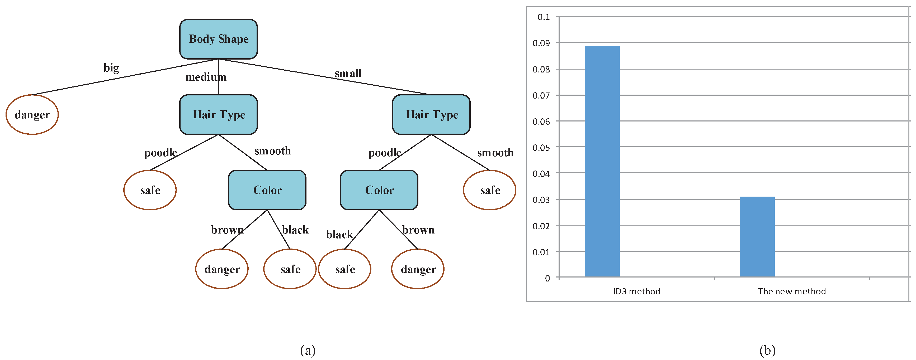
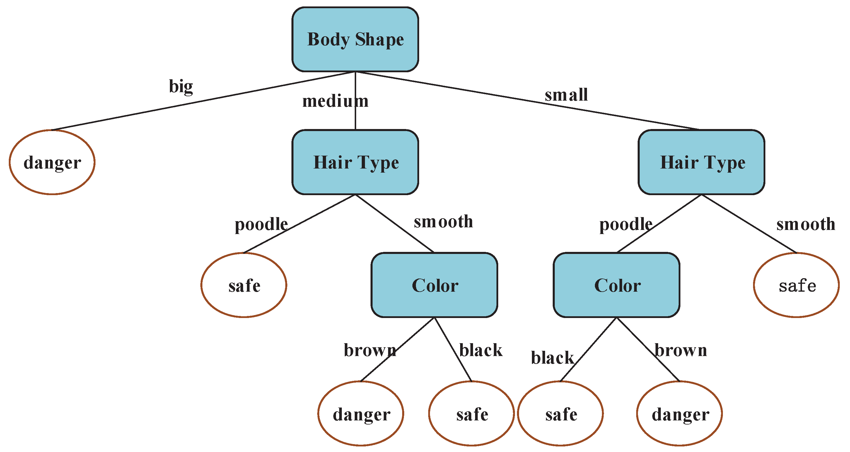
In order to verify the above theory, two decision trees are built based on the two different information gain equations (i.e., Equations (2) and (12)) for Table 1 to compare the length of running time about the two different methods.
The sample data in Table 1 is taken as the training set, and there are three candidate feature attributions (Color, Body Shape, Hair Type) and one class attribution (Characteristic) in this table. Although the decision trees that are built respectively based on the information gain Equations (2) and (12) are the same, which can be presented in Figure 2a, but the running time of the two solutions changed dramatically, which is shown in Figure 2b. The running time based on the new method is smaller than that of ID3, which is helpful for improving the real-time capability.
3.2. Variety Bias Problem and the Solution
People tend to choose as many attributes as possible to build decision tree models. If “Number” can be used as a candidate attribute, there will be four feature attributions (Number, Color, Body Shape, Hair Type) and one class attribution (characteristic) in Table 1. The selection of the optimal attribution based on Equations (2) and (12) presented above is the feature attribution “Number”, the detailed computation process is shown in the following. The decision tree model is presented in Figure 3. From Figure 3, we find that there is no sense to predict new samples for this decision tree, because each piece of sample data has their own number.
In order to avoid the multi-value bias problem, the C4.5 method used gain ratio instead of the information gain equation, which is a good solution to the multi-value bias problem, but more logarithmic expressions are brought into the computation process by gain ratio, which will influence the running time according to Section 3.1. This paper proposed a new method that introduces different weights for each attribute, which is not only helpful for the selection of the optimal attribution, but also brings no computation pressure. The detailed computation process based on the information gain equation in ID3 is shown in Equations (13)–(16). Equation (17) is the new information gain equation, and the computation process based on Equations (17) is also briefly listed in Equations (18)–(21). The decision tree built by the improved information gain equation is showed in Figure 4. Obviously, this decision tree has better prediction ability for new unknown samples than that of decision trees in Figure 3.
3.2.1. The Selection Process of the Optimal Attribution Based on the ID3 Method
The attribution that has the biggest information gain will be selected as the root node. From Equations (13)–(16), the attribution “Number” has the biggest information gain in Table 1. Hence, this attribution will be selected as the root node. Referring to Algorithm 1, the decision tree model is presented in Figure 3:
3.2.2. The Selection Process of the Optimal Attribution Based on the Improved Method
In order to solve the variety bias problem, different weights are introduced into each attribution based on Equation (17). Each weight equals the reciprocal of the length of different values in the corresponding attribution. The computation process is listed in the following:
The attribution that has the biggest information gain is the optimal attribution. If there is more than one property with the maximum information gain value, the optimal property will be randomly selected from these candidate attributions. The attribution “Body Shape” is finally randomly selected as the optimal attribution in Matlab, the decision tree model based on the improved method is presented in Figure 4.
With the help of Equation (8), a decision tree model will be quickly built and the problem of the variety bias problem will be avoided. This paper introduced the coordination degree theory to improve the feature of split points for acquiring a more concise decision tree model because the decision tree size is hard to control.
3.2.3. Uncontrollable Tree Size and the Solution
The splitting degree of internal node is hard to control, which will bring a lot of disadvantages, such as large tree size, long classification rules, and so on. Therefore, the concept of coordination degree is introduced in this paper, which plays a great role in determining the split property of the internal node in advance, and avoids the subsequent pruning step [36] that used to deal with the over-fitting problem. The basic idea of the proposed algorithm is that the standard of the splitting property of every branch is determined by the size of coordination degree and the condition certainty degree.
Assume that stands for training set, denotes condition attribute set, which is variable, and stands for the subset of a value in the attribute . denotes label attribute set, which is stationary.
Coordination degree is defined by:
The condition certainty degree is defined by:
The splitting property of different branches depends on the size of coordination degree and condition certainty degree in the subset. If the size of the coordination degree is greater than or equal to that of the coordination degree, the node will be a leaf node, on the contrary, the node will be an non-leaf node, which can continue be splitted.
The decision trees built by the two different methods are shown in Figure 5, and the right figure that has fewer nodes and branch rules is more concise than the left.
3.3. The Step of the Improved ID3 Algorithm
This paper presented a new method that combines the above three steps to build the decision tree. This new method could build a more concise decision tree in a shorter time by combining these three advantages than the ID3 method. The step of the improved ID3 algorithm is summarized in Algorithm 2.
| Algorithm 2: The improved algorithm based on ID3 method |
| Input: decision table |
| Output: a decision tree |
| 1 Generate node |
| 2 If the training sample inbelong to the same class. Then |
| 3 The node is labeled as leaf node named C; Return |
| 4 End if |
| 5 If or the values in A are same in D, Then |
| 6 The node is labeled as leaf node; Return |
| 7 Else |
| 8 Minimum entropy is chosen as a heuristic strategy to select the optimal partition attribute from A based on the simplified information gain; |
| 9 For every value in do |
| 10 Generate a branch for node; is the sample subset that has value from in D |
| 11 If is empty. Then |
| 12 The node in a branch is labeled as a leaf node; Return |
| 13 Else |
| 14 Forevery branch of do |
| 15 Determine split property by comparing the size of the coordination degree and condition certainty degree. |
| 16 If or there are no other condition attributes, define the branch as a leaf node. |
| 17 ELSE define the branch as a none-leaf node, return Step 8. |
| 18 End if |
| 19 End for |
| 20 End if |
| 21 End for |
| 22 End if |
4. The Assessment of the Decision Tree Algorithm
In general, the improved solutions can be obtained by assessing the generalization error of the existed decision tree models. Hence, the step of choosing a reasonable assessment algorithm is necessary. The main purpose of the assessment algorithm is to judge the accuracy of the mathematical model.
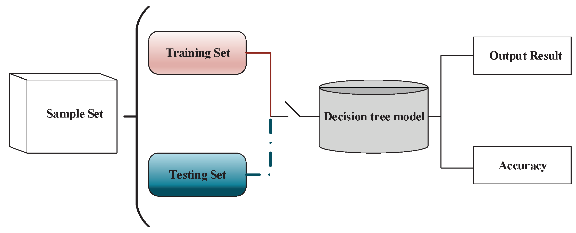
There are many assessment algorithms [37,38,39] such as a hold-out algorithm, cross validation algorithm and bootstrapping algorithm. The last two algorithms are more common in the case of enough data. This paper selected the first algorithm (hold-out algorithm) as the assessment algorithm to judge the validity of a decision tree model due to its rapidity and convenience. The detailed procedure of the hold-out algorithm is shown in Figure 6. How can we have the training set and the testing set from the data set D? This paper used the first method to divide D into two parts: one is used as training set, and the other is used as a testing set.
5. Examples and Analyses
Three examples are used to verify the feasibility of the new method in Section 3.3, and all example results have proved the effectiveness and viability of the optimized scheme.
5.1. Example 1
The data set depicted in Table 1 is obtained from common life, which is used to judge the family dogs’ characteristics based on the three attributes (Body Shape, Hair Type, Colour). The samples in Table 1 are randomly divided into two subsets (training set and testing set). There are nine samples in the training set, which are acquired by the function command (a = randperm(12), Train = data(a(1:9),:), Test = data(a(10:end),:) in Matlab.
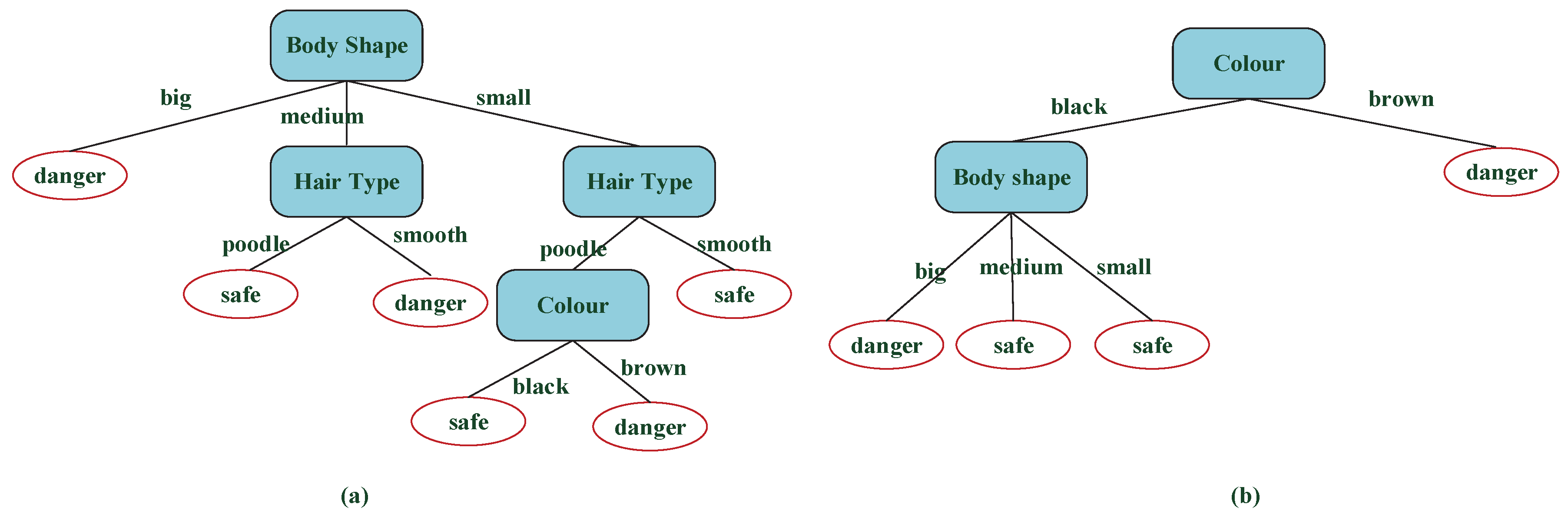
Two different decision tree models about family dogs’ characteristics are built based on the training set that depicted in Table 2, and the two models are finally listed in Figure 7.
From Figure 7a,b, the decision tree model built by the improved algorithm is more concise, which can also be displayed in classification rules. The decision tree model in Figure 7a that built by the ID3 algorithm produces 10 nodes and 6 rules:
- 1
- if Body shape = big, then class = danger;
- 2
- if Body shape = medium and Hair type = poodle, then Characteristic = safe;
- 3
- if Body shape = medium and Hair type = smooth, then Characteristic = danger;
- 4
- if Body shape = small and Hair type = poodle, and Colour = black, then Characteristic = safe;
- 5
- if Body shape = small and Hair type = poodle, and Colour = brown, then Characteristic = danger;
- 6
- if Body shape = small and Hair type = smooth, then Characteristic = safe.
The decision tree built by the improved ID3 algorithm produces six nodes and four rules, and all rules are listed as the following:
- 1
- if Colour = black, Body shape = big, then Characteristic = danger;
- 2
- if Colour = black, Body shape = medium, then Characteristic = safe;
- 3
- if Colour = black, Body shape = small, then Characteristic = safe;
- 4
- if Colour = brown, then Characteristic = danger.
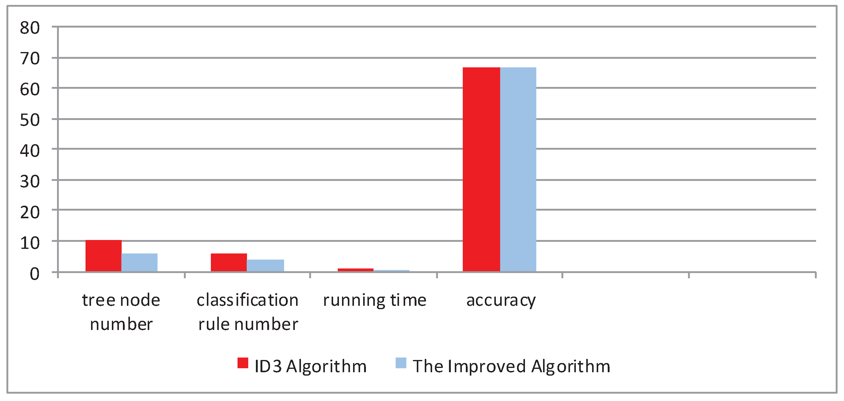
The optimal attribute of the root node in Figure 7a is Body Shape that has three values, but the optimal attribute of the root node in Figure 7b is color that has two values, which solves the attribution bias problem. The accuracy of the testing set can be predicted by the above rules. After testing, all differences of the two decision tree models shown in Figure 7 are summarized in Table 3 and Figure 8.
5.2. Example 2
Referring to a decision table depicted in Table 2, which relates the decisions of playing balls based on weather conditions, where is the collection of 24 objects. The attribute set is a condition attribute unit, and the attribute set is a label attribute set. There are two data sets (i.e., training set and testing set ), which are randomly divided according to Table 2 through the function command (a = randperm(24); Train = data(a(1:17),:); Test = data(a(18:end),:) in Matlab. There are 17 samples in the training set, which includes 8 N and 9 Y , and seven samples in the testing set, which includes 4 N and 3 Y. The data of the training set and the data of the testing set are presented in Table 4. Next, a decision tree model of the event in Table 4 will be built based on ID3 and the new method, and the two decision tree models are listed in Figure 9.
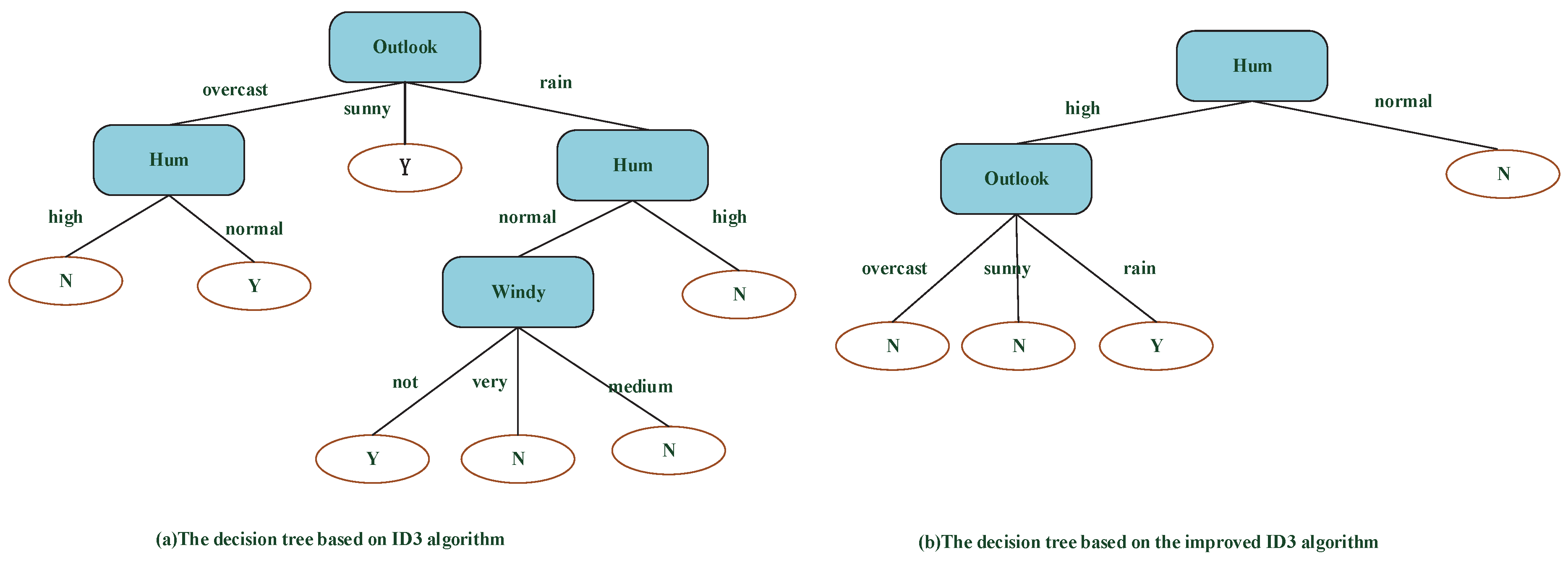
From Figure 9a,b, the decision tree model built by the improved algorithm is more concise. The decision tree built by the ID3 algorithm produces 11 nodes and seven rules:
- 1
- if Outlook = overcast and Hum = high, then d = N;
- 2
- if Outlook = overcast and Hum = normal, then d = Y;
- 3
- if Outlook = sunny, then d = Y;
- 4
- if Outlook = rain, Hum = normal, then Windy = not, then d = Y;
- 5
- if Outlook = rain, Hum = normal, then Windy = very, then d = N;
- 6
- if Outlook = rain, Hum = normal, then Windy = medium, then d = N;
- 7
- if Outlook = rain, Hum = high, then d = N.
The decision tree built by the improved ID3 algorithm produces six nodes and four rules:
- 1
- if Hum = high, Outlook = overcast, then d = N;
- 2
- if Hum = high, Outlook = sunny, then d = N;
- 3
- if Hum = high, Outlook = rain, then d = Y;
- 4
- if Hum = normal, then d = N.
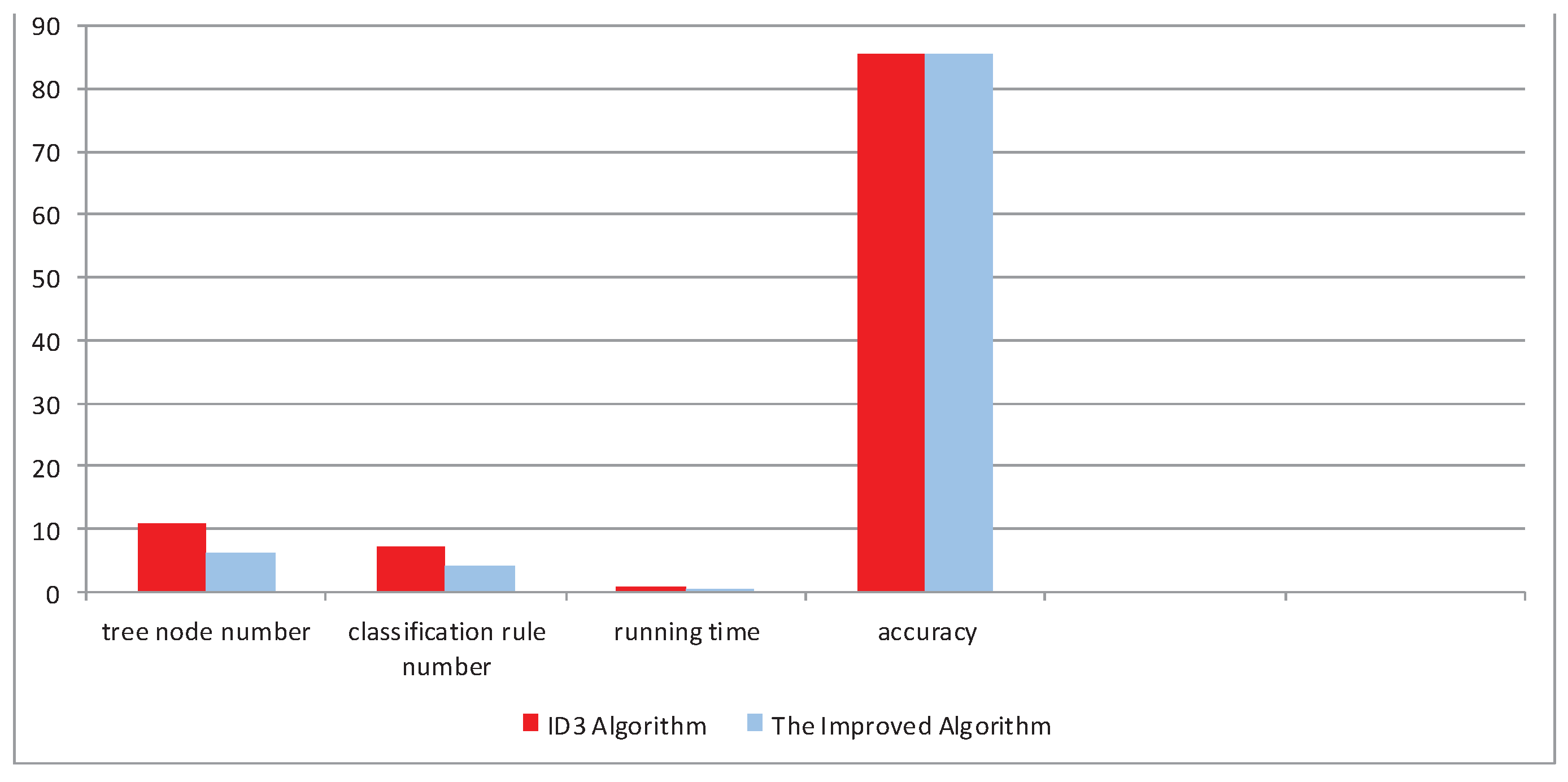
The latter has a smaller scale and shorter rules by contrast. The accuracy of the improved ID3 algorithm equals that of the ID3 method (i.e., 85.71%) after predicting the labels of testing samples. The running time (i.e., 0.073 s) of the improved method is shorter than that (i.e., 0.769 s) of the ID3 algorithm, and the tree size built by the improved algorithm is more concise than that of the ID3 method. The optimal attribute of root node in Figure 9a is Outlook that has three values (the maximum number of all attributions), but the optimal attribute of root node in Figure 9b is hum that has two values, which proves that the attribute that has multi-values is not always the optimal attribute. All differences between the ID3 algorithm and the improved ID3 algorithm are summarized in Table 5 and Figure 10.
5.3. Example 3
Examples 1 and 2 verified the effectiveness and availability of the optimized scheme well, but the sample sizes of the first two examples are too small to prove the extensibility of the proposed method, especially in accuracy. In order to highlight the differences of the two methods, this paper downloaded Wisconsin Breast Cancer Database [40] that includes 699 samples from the University of Californiairvine (UCI) machine learning database. This database is collected and denoted to Machine learning problem library by William H. Wolberg from the University of Wisconsin-Madison.
Each case in the sample set was performed with a cytological examination and postoperative pathological examination. There are nine feature attributions (Clump Thickness, Uniformity of Cell Size, Uniformity of Cell Shape, Marginal Adhesion, Single Epithelial Cell Size, Bare Nucleoli Bland Chromatin, Normal Nucleoli and Mitoses) and one label attribution that including two classes: benign and malignant in this database. In this data sample, there are 241 malignant and 458 benign. The training sample set that includes 500 examples was selected randomly from the 699 examples, the other samples were selected as the testing set.
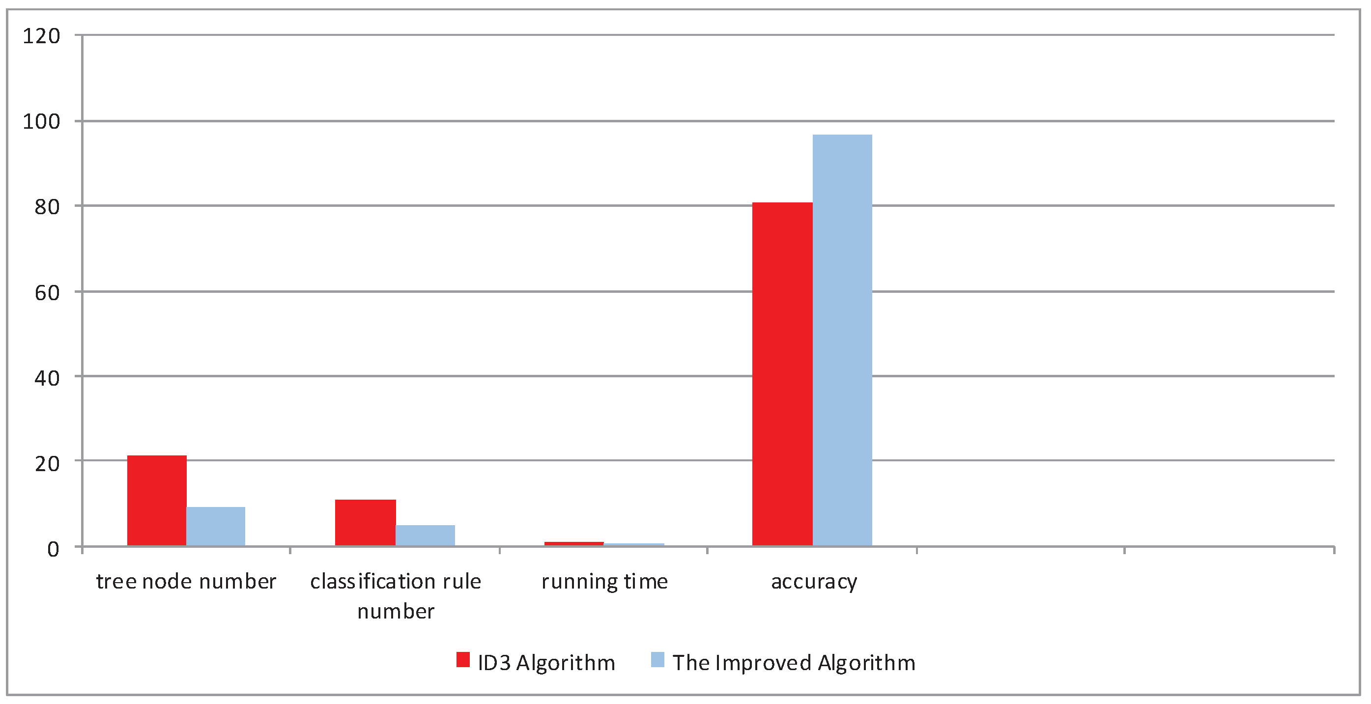
Two different decision trees based on the two methods are listed in Figure 11, and, obviously, the decision tree model built by the new method is more concise than that of the ID3 method, which is verified from the experimental results. All differences between the ID3 algorithm and the improved ID3 algorithm are summarized in Table 6 and Figure 12.
6. Conclusions
This paper proposed an improved ID3 algorithm, in which the information entropy equation that includes addition, subtraction, multiplication, and division firstly replaced the original information entropy expression that includes complicated logarithm operation in the ID3 method for economizing large amounts of running time, and then different weight values are respectively added to the new information entropy expression of each attribution for overcoming the multi-value bias problem in the ID3 method. Finally, the coordination degree is introduced to control the splitting degree of each internal node for building a more concise decision tree. The results of these experiments clearly indicate that the new algorithm in this study leads to less running time, shorter decision rules and higher predictive accuracy than those of the ID3 algorithm.
For future work, we will study how to build classifiers for dynamic data samples because they are more common than static samples in our life. We will also study how to choose a more efficient assessment method for reasonably assigning the training set and the testing set in view of its importance to the predictive accuracy of the decision tree model.
Acknowledgments
This work was supported by the National Nature Science Foundation of China Grant Nos. 61673245, 61573213 and 61703243.
Author Contributions
Yibin Li and Yingying Wang conceived the research and conducted the simulations; Yingying Wang designed and implemented the algorithm; Yong Song analyzed the data, results and verified the theory; Xuewen Rong and Shuaishuai Zhang collected a large number of references and suggested some good ideas about this paper; all authors participated in the writing of the manuscript.
Conflicts of Interest
The authors declare no conflict of interest.
References
- Kirkos, E.; Spathis, C.; Manolopoulos, Y. Data Mining techniques for the detection of fraudulent financial statements. Exp. Syst. Appl. 2007, 32, 995–1003. [Google Scholar] [CrossRef]
- Witten, I.H.; Frank, E. Data Mining: Practical Machine Learning Tools and Techniques with Java Implementations; Morgan Kaufmann Publisher: Dordrecht, The Netherlands, 2000; Volume 31, pp. 76–77. [Google Scholar]
- Gandhi, M.; Singh, S.N. Predictions in Heart Disease Using Techniques of Data Mining. In Proceedings of the International Conference on Futuristic Trends on Computational Analysis and Knowledge Management, Noida, India, 25–27 Feburary 2015; pp. 520–525. [Google Scholar]
- Vishnubhotla, P.R. Storing Data Mining Clustering Results in a Relational Database for Querying and Reporting. U.S. Patent 6,718,338, 6 April 2004. [Google Scholar]
- Hall, M.A.; Holmes, G. Benchmarking Attribute Selection Techniques for Discrete Class Data Mining. IEEE Trans. Knowl. Data Eng. 2003, 15, 1437–1447. [Google Scholar] [CrossRef]
- Thabtah, F. A review of associative classification mining. Knowl. Eng. Rev. 2007, 22, 37–65. [Google Scholar] [CrossRef]
- Codenotti, B.; Leoncini, M. Parallelism and fast solution of linear systems. Comput. Math. Appl. 1990, 19, 1–18. [Google Scholar] [CrossRef]
- Huang, C.J.; Yang, D.X.; Chuang, Y.T. Application of wrapper approach and composite classifier to the stock trend prediction. Exp. Syst. Appl. 2008, 34, 2870–2878. [Google Scholar] [CrossRef]
- Tsai, C.F.; Lin, Y.C.; Yen, D.C.; Chen, Y.M. Predicting stock returns by classifier ensembles. Appl. Comput. 2011, 11, 2452–2459. [Google Scholar] [CrossRef]
- Ahmadi, A.; Omatu, S.; Kosaka, T. A PCA Based Method for Improving the Reliability of Bank Note Classifier Machines. In Proceedings of the International Symposium on Image and Signal Processing and Analysis, Rome, Italy, 18–20 September 2003; Volume 1, pp. 494–499. [Google Scholar]
- Ozkan-Gunay, E.N.; Ozkan, M. Prediction of bank failures in emerging financial markets: An ANN approach. J. Risk Financ. 2007, 8, 465–480. [Google Scholar] [CrossRef]
- Tarter, R.E. Evaluation and treatment of adolescent substance abuse: A decision tree method. Am. J. Drug Alcohol. Abus. 1990, 16, 1–46. [Google Scholar] [CrossRef]
- Sekine, S.; Grishman, R.; Shinnou, H. A Decision Tree Method for Finding and Classifying Names in Japanese Texts. In Proceedings of the Sixth Workshop on Very Large Corpora, Montreal, QC, Canada, 15–16 August 1998. [Google Scholar]
- Carpenter, G.A.; Grossberg, S.; Reynolds, J.H. ARTMAP: Supervised real-time learning and classification of nonstationary data by a self-organizing neural network. Neural Netw. 1991, 4, 565–588. [Google Scholar] [CrossRef]
- Vukasinovi, M.; Djuki, V.; Stankovi, P.; Krejovi-Trivi, S.; Trivi, A.; Pavlovi, B. International Statistical Classification of Diseases and Related Health Problems. Acta Chir. Iugosl. 2009, 56, 65–69. [Google Scholar] [CrossRef]
- Brockwell, S.E.; Gordon, I.R. A comparison of statistical methods for meta-analysis. Stat. Med. 2001, 20, 825–840. [Google Scholar] [CrossRef] [PubMed]
- Phu, V.N.; Tran, V.T.N.; Chau, V.T.N.; Dat, N.D.; Duy, K.L.D. A decision tree using ID3 algorithm for English semantic analysis. Int. J. Speech Technol. 2017, 20, 593–613. [Google Scholar] [CrossRef]
- Elomaa, T. In Defense of C4.5: Notes on Learning One-Level Decision Trees. Mach. Learn. Proc. 1994, 254, 62–69. [Google Scholar]
- Lawrence, R.L. Rule-Based Classification Systems Using Classification and Regression Tree (CART) Analysis. Photogr. Eng. Remote Sens. 2001, 67, 1137–1142. [Google Scholar]
- Hssina, B.; Merbouha, A.; Ezzikouri, H.; Erritali, M. A comparative study of decision tree ID3 and C4.5. Int. J. Adv. Comput. Sci. Appl. 2014, 4, 13–19. [Google Scholar] [CrossRef]
- Al-Sarem, M. Predictive and statistical analyses for academic advisory support. arXiv, 2015; arXiv:1601.04244. [Google Scholar]
- Lerman, R.I.; Yitzhaki, S. A note on the calculation and interpretation of the Gini index. Econ. Lett. 1984, 15, 363–368. [Google Scholar] [CrossRef]
- Fayyad, U.M.; Irani, K.B. The Attribute Selection Problem in Decision Tree Generation. In Proceedings of the National Conference on Artificial Intelligence, San Jose, CA, USA, 12–16 July 1992; pp. 104–110. [Google Scholar]
- LIANG, J.; SHI, Z. The Information Entropy, Rough Entropy and Knowledge Granulation in Rough Set Theory. Int. J. Uncertain. Fuzziness Knowl.-Based Syst. 2008, 12, 37–46. [Google Scholar] [CrossRef]
- Exarchos, T.P.; Tsipouras, M.G.; Exarchos, C.P.; Papaloukas, C.; Fotiadis, D.I.; Michalis, L.K. A methodology for the automated creation of fuzzy expert systems for ischaemic and arrhythmic beat classification based on a set of rules obtained by a decision tree. Artif. Intell. Med. 2007, 40, 187–200. [Google Scholar] [CrossRef] [PubMed]
- Quinlan, J.R. Generating Production Rules from Decision Trees. In Proceedings of the International Joint Conference on Artificial Intelligence, Cambridge, MA, USA, 23–28 August 1987; pp. 304–307. [Google Scholar]
- Sneyers, J.; Schrijvers, T.; Demoen, B. The computational power and complexity of Constraint Handling Rules. In Proceedings of the 2nd Workshop on Constraint Handling Rules, Sitges, Spain, 2–5 October 2005; pp. 3–17. [Google Scholar]
- Lei, S.P.; Xie, J.C.; Huang, M.C.; Chen, H.Q. Coordination degree analysis of regional industry water use system. J. Hydraul. Eng. 2004, 5, 1–7. [Google Scholar]
- Zhang, P.; Su, F.; Li, H.; Sang, Q. Coordination Degree of Urban Population, Economy, Space, and Environment in Shenyang Since 1990. China Popul. Resour. Environ. 2008, 18, 115–119. [Google Scholar]
- Parmar, D.; Wu, T.; Blackhurst, J. MMR: An algorithm for clustering categorical data using Rough Set Theory. Data Knowl. Eng. 2007, 63, 879–893. [Google Scholar] [CrossRef]
- Quinlan, J.R. Induction of Decision Trees; Kluwer Academic Publishers: Dordrecht, The Netherlands, 1986; pp. 81–106. [Google Scholar]
- Arif, F.; Suryana, N.; Hussin, B. Cascade Quality Prediction Method Using Multiple PCA+ID3 for Multi-Stage Manufacturing System. Ieri Procedia 2013, 4, 201–207. [Google Scholar] [CrossRef]
- De Mántaras, R.L. A Distance-Based Attribute Selection Measure for Decision Tree Induction. Mach. Learn. 1991, 6, 81–92. [Google Scholar] [CrossRef]
- Coleman, J.N.; Chester, E.I.; Softley, C.I.; Kadlec, J. Arithmetic on the European logarithmic microprocessor. IEEE Trans. Comput. 2001, 49, 702–715. [Google Scholar] [CrossRef]
- Leung, C.S.; Wong, K.W.; Sum, P.F.; Chan, L.W. A pruning method for the recursive least squared algorithm. Neural Netw. 2001, 14, 147. [Google Scholar] [CrossRef]
- Yang, T.; Gao, X.; Sorooshian, S.; Li, X. Simulating California reservoir operation using the classification and regression-tree algorithm combined with a shuffled cross-validation scheme. Water Resour. Res. 2016, 52, 1626–1651. [Google Scholar] [CrossRef]
- Kohavi, R. A study of Cross-Validation and Bootstrap for Accuracy Estimation And Model Selection. In Proceedings of the International Joint Conference on Artificial Intelligence, Montreal, QC, Canada, 20–25 August 1995; pp. 1137–1143. [Google Scholar]
- Kim, J.H. Estimating classification error rate: Repeated cross-validation, repeated hold-out and bootstrap. Comput. Stat. Data Anal. 2009, 53, 3735–3745. [Google Scholar] [CrossRef]
- Refaeilzadeh, P.; Tang, L.; Liu, H. Cross-Validation. In Encyclopedia of Database Systems; Springer: New York, NY, USA, 2016; pp. 532–538. [Google Scholar]
- Mumtaz, K.; Sheriff, S.A.; Duraiswamy, K. Evaluation of three neural network models using Wisconsin breast cancer database. In Proceedings of the International Conference on Control, Automation, Communication and Energy Conservation, Perundurai, India, 4–6 June 2009; pp. 1–7. [Google Scholar]
Figure 1.
The tree chart of a decision tree.
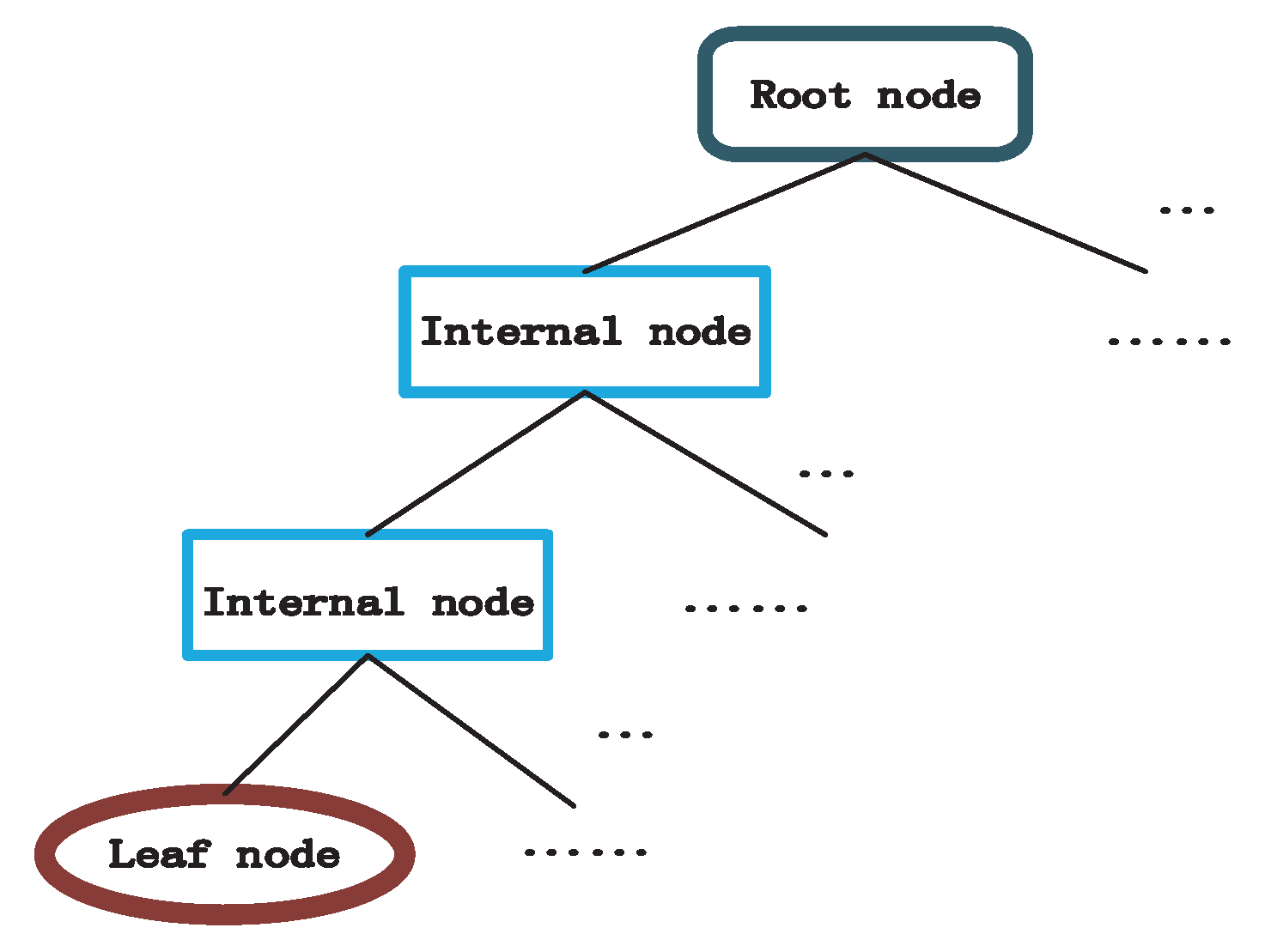
Figure 2.
Comparison in building a same decision tree model: (a) the decision tree model based on ID3 and the new method; (b) the comparison of running time about ID3 and the new method.
Figure 2.
Comparison in building a same decision tree model: (a) the decision tree model based on ID3 and the new method; (b) the comparison of running time about ID3 and the new method.

Figure 3.
Decision tree model based on ID3 method.
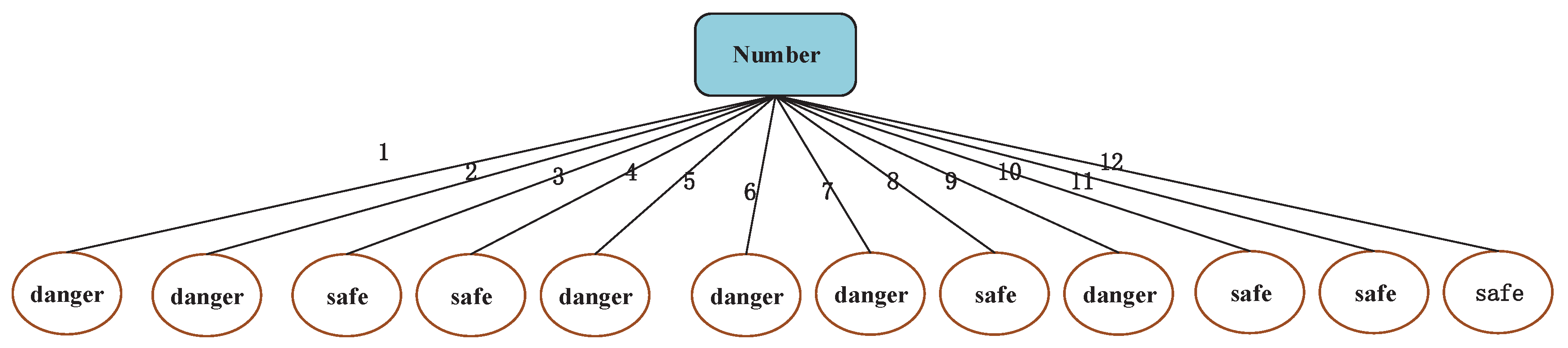
Figure 4.
Decision tree model based on the improved method.

Figure 5.
Different tree structures based on ID3 and the new method: (a) the decision tree based on ID3 method; (b) the decision tree based on the new method.
Figure 5.
Different tree structures based on ID3 and the new method: (a) the decision tree based on ID3 method; (b) the decision tree based on the new method.
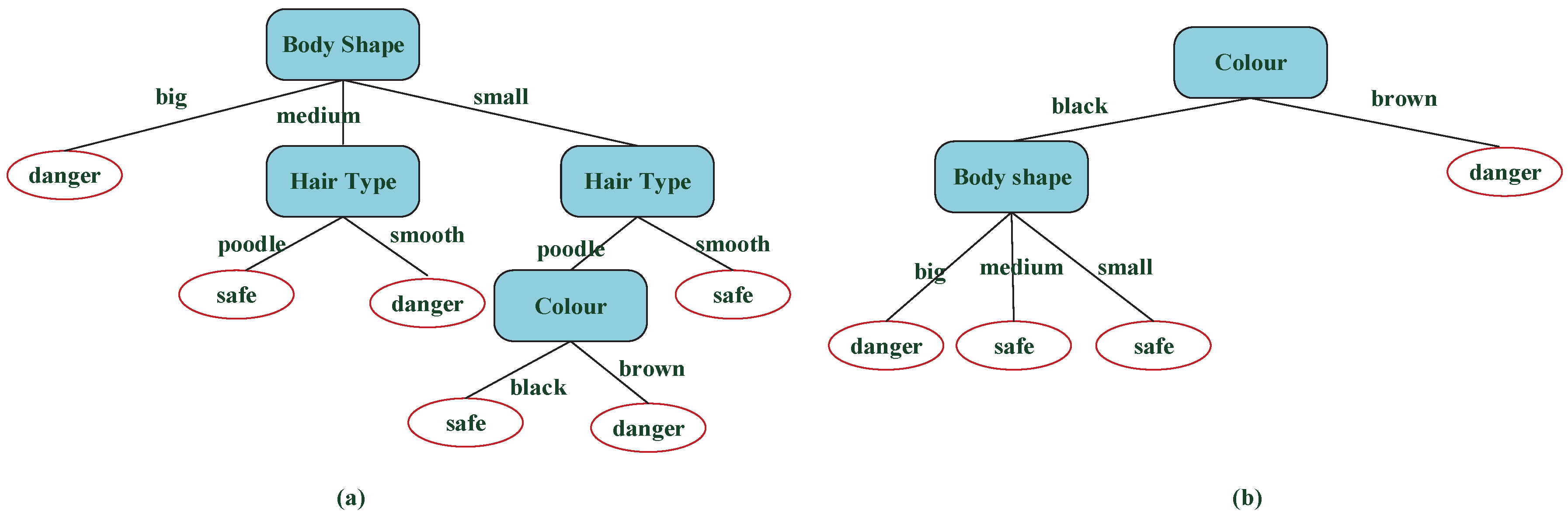
Figure 6.
The process of assessing a decision tree.

Figure 7.
Decision tree models using different algorithms based on family dogs’ characteristics: (a) the decision tree using ID3 algorithm; (b) the decision tree using the improved algorithm based on ID3 method.
Figure 7.
Decision tree models using different algorithms based on family dogs’ characteristics: (a) the decision tree using ID3 algorithm; (b) the decision tree using the improved algorithm based on ID3 method.

Figure 8.
Bar chart comparison results by two different methods based on Table 3.
Figure 8.
Bar chart comparison results by two different methods based on Table 3.

Figure 9.
Decision tree models based on weather using two different algorithms: (a) the decision tree model using ID3 method; (b) the decision tree model using the improved algorithm based on ID3 method.
Figure 9.
Decision tree models based on weather using two different algorithms: (a) the decision tree model using ID3 method; (b) the decision tree model using the improved algorithm based on ID3 method.

Figure 10.
Bar chart comparison results by the ID3 method and the new method based on Table 5.
Figure 10.
Bar chart comparison results by the ID3 method and the new method based on Table 5.

Figure 11.
Decision tree models based on the cancer label using different algorithms: (a) the decision tree model using ID3 method; (b) the decision tree model using the improved algorithm based on ID3 method.
Figure 11.
Decision tree models based on the cancer label using different algorithms: (a) the decision tree model using ID3 method; (b) the decision tree model using the improved algorithm based on ID3 method.
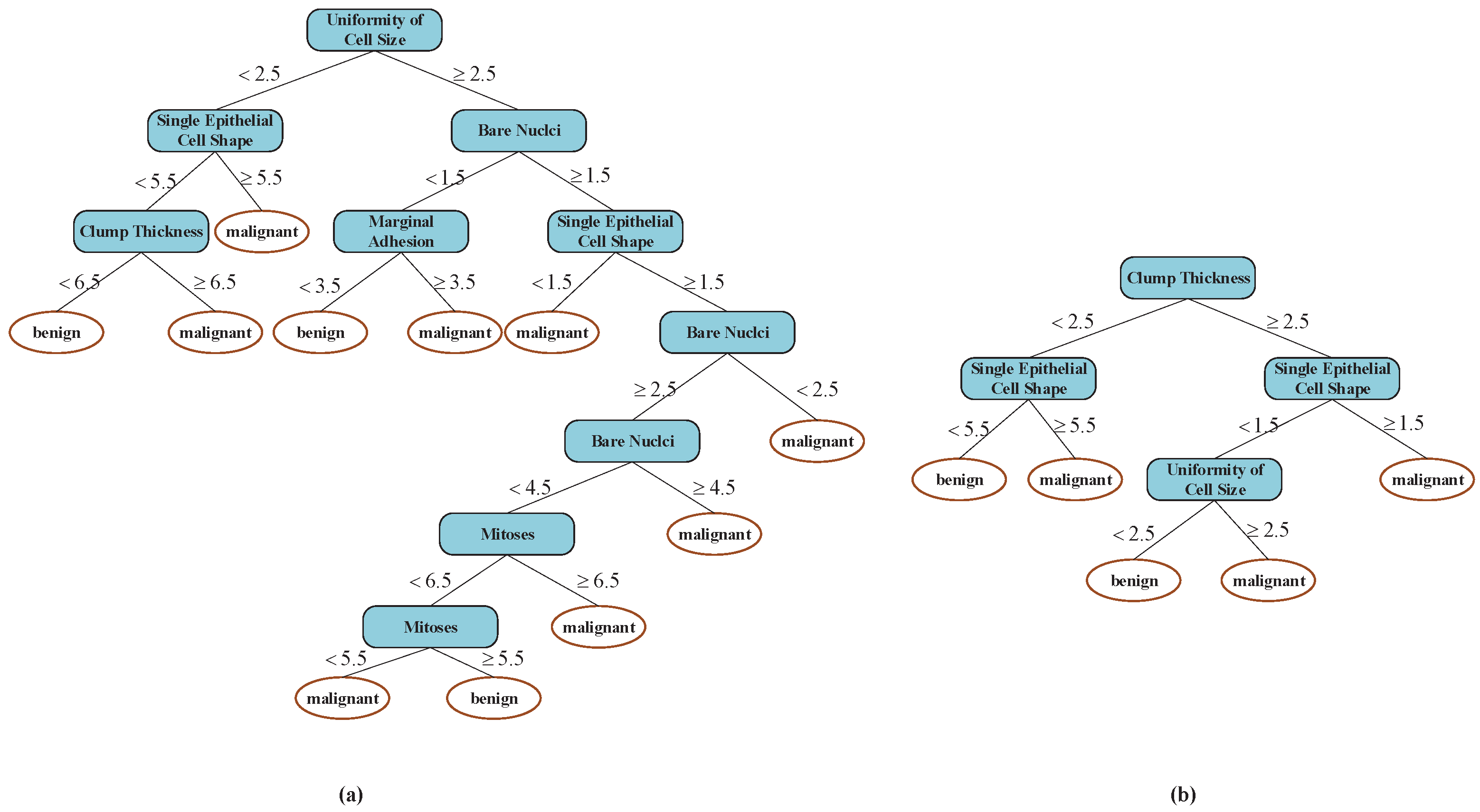
Figure 12.
Bar chart comparison results by the ID3 method and the new method based on Table 6.
Figure 12.
Bar chart comparison results by the ID3 method and the new method based on Table 6.


Table 1.
The data sample that determines the risk of dogs.
| Number | Colour | Body Shape | Hair Type | Characteristic |
|---|---|---|---|---|
| 1 | black | big | poodle | danger |
| 2 | brown | big | smooth | danger |
| 3 | brown | medium | poodle | safe |
| 4 | black | small | poodle | safe |
| 5 | brown | medium | smooth | danger |
| 6 | black | big | smooth | danger |
| 7 | brown | small | poodle | danger |
| 8 | brown | small | smooth | safe |
| 9 | brown | big | poodle | danger |
| 10 | black | medium | poodle | safe |
| 11 | black | medium | smooth | safe |
| 12 | black | small | smooth | safe |
Table 2.
Experimental dataset based on family dogs’ characteristic.
| Training Set | ||||
|---|---|---|---|---|
| Number | Colour | Body Shape | Hair Type | Characteristic |
| 1 | black | big | poodle | danger |
| 2 | brown | big | smooth | danger |
| 4 | black | small | poodle | safe |
| 5 | brown | medium | smooth | danger |
| 7 | brown | small | poodle | danger |
| 8 | brown | small | smooth | safe |
| 9 | brown | big | poodle | danger |
| 10 | black | medium | poodle | safe |
| 12 | black | small | smooth | safe |
| Testing Set | ||||
| Number | Colour | Body Shape | Hair Type | Characteristic |
| 3 | brown | medium | poodle | safe |
| 6 | black | big | smooth | danger |
| 11 | black | medium | smooth | safe |
Table 3.
Experimental results by the ID3 method and the new method based on family dogs’ characteristics.
Table 3.
Experimental results by the ID3 method and the new method based on family dogs’ characteristics.
| Algorithm | Tree Node Number | Classification Rule Number | Running Time | Accuracy (%) |
|---|---|---|---|---|
| ID3 Algorithm | 10 | 6 | 0.778 | 66.7 |
| The Improved Algorithm | 6 | 4 | 0.107 | 66.7 |
Table 4.
Experimental dataset based on the decision of playing tennis.
| Training Set | |||||
|---|---|---|---|---|---|
| Number | Outlook | Term | Hum | Windy | d |
| 1 | overcast | hot | high | not | N |
| 2 | overcast | hot | high | very | N |
| 3 | overcast | hot | high | medium | N |
| 5 | sunny | hot | high | medium | Y |
| 6 | rain | mild | high | not | N |
| 7 | rain | mild | high | medium | N |
| 8 | rain | hot | normal | not | Y |
| 9 | rain | cool | normal | medium | N |
| 10 | rain | hot | normal | very | N |
| 12 | sunny | cool | normal | medium | Y |
| 13 | overcast | mild | high | not | N |
| 15 | overcast | cool | normal | medium | Y |
| 17 | rain | mild | normal | not | N |
| 22 | sunny | mild | high | medium | Y |
| 24 | rain | mild | high | very | N |
| 20 | overcast | mild | normal | very | Y |
| 21 | sunny | mild | high | very | Y |
| 23 | sunny | hot | normal | not | Y |
| Testing Set | |||||
| Number | Outlook | Term | Hum | Windy | d |
| 11 | sunny | cool | normal | very | Y |
| 14 | overcast | mild | high | medium | N |
| 16 | overcast | cool | normal | medium | Y |
| 18 | rain | mild | normal | medium | N |
| 19 | overcast | mild | normal | medium | Y |
Table 5.
Results by the ID3 method and the new method based on the decision of playing tennis.
| Algorithm | Tree Node Number | Classification Rule Number | Running Time | Accuracy (%) |
|---|---|---|---|---|
| ID3 Algorithm | 11 | 7 | 0.769 | 85.71 |
| The Improved Algorithm | 6 | 4 | 0.073 | 85.71 |
Table 6.
Experimental results by the ID3 method and the new method based on the cancer label.
| Algorithm | Tree Node Number | Classification Rule Number | Running Time | Accuracy (%) |
|---|---|---|---|---|
| ID3 Algorithm | 21 | 11 | 0.899 | 80.49 |
| The Improved Algorithm | 9 | 5 | 0.368 | 96.52 |
© 2017 by the authors. Licensee MDPI, Basel, Switzerland. This article is an open access article distributed under the terms and conditions of the Creative Commons Attribution (CC BY) license (http://creativecommons.org/licenses/by/4.0/).
Share and Cite
MDPI and ACS Style
Wang, Y.; Li, Y.; Song, Y.; Rong, X.; Zhang, S. Improvement of ID3 Algorithm Based on Simplified Information Entropy and Coordination Degree. Algorithms 2017, 10, 124. https://doi.org/10.3390/a10040124
AMA Style
Wang Y, Li Y, Song Y, Rong X, Zhang S. Improvement of ID3 Algorithm Based on Simplified Information Entropy and Coordination Degree. Algorithms. 2017; 10(4):124. https://doi.org/10.3390/a10040124
Chicago/Turabian StyleWang, Yingying, Yibin Li, Yong Song, Xuewen Rong, and Shuaishuai Zhang. 2017. "Improvement of ID3 Algorithm Based on Simplified Information Entropy and Coordination Degree" Algorithms 10, no. 4: 124. https://doi.org/10.3390/a10040124
Note that from the first issue of 2016, this journal uses article numbers instead of page numbers. See further details here.