Truss Structure Optimization with Subset Simulation and Augmented Lagrangian Multiplier Method

1
Aircraft Strength Research Institute of China, Xi’an 710065, China
2
College of Aerospace Engineering, Nanjing University of Aeronautics and Astronautics, Nanjing 210016, China
*
Author to whom correspondence should be addressed.
Algorithms 2017, 10(4), 128; https://doi.org/10.3390/a10040128
Submission received: 20 August 2017
/
Revised: 10 November 2017
/
Accepted: 12 November 2017
/
Published: 21 November 2017
Abstract
:This paper presents a global optimization method for structural design optimization, which integrates subset simulation optimization (SSO) and the dynamic augmented Lagrangian multiplier method (DALMM). The proposed method formulates the structural design optimization as a series of unconstrained optimization sub-problems using DALMM and makes use of SSO to find the global optimum. The combined strategy guarantees that the proposed method can automatically detect active constraints and provide global optimal solutions with finite penalty parameters. The accuracy and robustness of the proposed method are demonstrated by four classical truss sizing problems. The results are compared with those reported in the literature, and show a remarkable statistical performance based on 30 independent runs.
1. Introduction
In modern design practice, structural engineers are often faced with structural optimization problems, which aim to find an optimal structure with minimum weight (or cost) under multiple general constraints, e.g., displacement, stress, or bulking limits, etc. It is theoretically straightforward to formulate the structural optimization problem as a constrained optimization problem in terms of equations under the framework of mathematical programming. This, however, is very challenging to accomplish in practice, at least, due to three reasons: (a) the number of design variables is large; (b) the feasible region is highly irregular; and (c) the number of design constraints is large.
Flexible optimization methods, which are able to deal with multiple general constraints that may have non-linear, multimodal, or even discontinuous behaviors, are desirable to explore complex design spaces and find the global optimal design. Optimization methods can be roughly classified into two groups: gradient-based methods and gradient-free methods. Gradient-based methods use the gradient information to search the optimal design starting from an initial point [1]. Although these methods have been often employed to solve structural optimization problems, solutions may not be good if the optimization problem is complex, particularly when the abovementioned major difficulties are involved. An alternative could be the deterministic global optimization methods, e.g., the widely used DIRECT method [2,3], which is a branch of gradient-free methods. Recently, Kvasov and his colleagues provided a good guide on the deterministic global optimization methods [4] and carried out a comprehensive comparison study between the deterministic and stochastic global optimization methods for one-dimensional problems [5]. One of the main disadvantages of the deterministic global optimization methods is the high-dimensionality issue caused by the larger number of design variables [3] or constraints. In contrast, another branch of gradient-free methods (or stochastic optimization methods), such as Genetic Algorithms (GA) [6,7,8,9,10,11,12], Simulated Annealing (SA) [13,14,15], Ant Colony Optimization (ACO) [16,17,18,19], Particle Swarm Optimizer (PSO) [17,20,21,22,23,24,25,26,27], Harmony Search (HS) [28,29,30,31], Charged System Search (CSS) [32], Big Bang-Big Crunch (BB-BC) [33], Teaching–Learning based optimization (TLBO) [34,35], Artificial Bee Colony optimization (ABC-AP) [36], Cultural Algorithm (CA) [37], Flower Pollination Algorithm (FPA) [38], Water Evaporation Optimization (WEO) [39], and hybrid methods combining two or more stochastic methods [40,41] have been developed to find the global optimal designs for both continuous and discrete structural systems. They have been attracting increasing attention for structural optimization because of their ability to overcome the drawbacks of gradient-based optimization methods and the high-dimensionality issue. A comprehensive review of stochastic optimization of skeletal structures was provided by Lamberti and Pappalettere [42]. All of the stochastic optimization methods share a common feature, that is, they are inspired by the observations of random phenomena in nature. For example, GA mimics natural genetics and the survival-of-the-fittest code. To implement a stochastic optimization method, random manipulation plays the key role to “jump” out local optima, such as the crossover and mutation in GA, the random velocity and position in PSO, etc. Although these stochastic optimization methods have achieved many applications in structural design optimization, structural engineers are still concerned with seeking more efficient and robust methods because no single universal method is capable of handling all types of structural optimization problems.
This paper aims to propose an efficient and robust structural optimization method that combines subset simulation optimization (SSO) and the augmented Lagrangian multiplier method [43]. In our previous studies [44,45,46], a new stochastic optimization method using subset simulation—the so-called subset simulation optimization (SSO)—was developed for both unconstrained and constrained optimization problems. Compared with some well-known stochastic methods, it was found to be promising for exploiting the feasible regions and searching optima for complex optimization problems. Subset simulation was originally developed for reliability problems with small failure probabilities, and then became a well-known simulation-based method in the reliability engineering community [47,48]. By introducing artificial probabilistic assumptions on design variables, the objective function maps the multi-dimensional design variable space into a one-dimensional random variable space. Due to the monotonically non-decreasing and right-continuous characteristics of the cumulative distribution function of a real-valued random variable, the searching process for optimized design(s) in a global optimization problem is similar to the exploring process for the tail region of the response function in a reliability problem [44,45,46].
The general constraints in structural optimization problems should be carefully handled. Since most stochastic optimization methods have been developed as unconstrained optimizers, common or special constraint-handling methods are required [49]. A modified feasibility-based rule has been proposed to deal with multiple constraints in SSO [45]. However, the rule fails to directly detect active constraints. As an enhancement, the dynamic augmented Lagrangian multiplier method (DALMM) [25,26,50] is presented and integrated with SSO for the constrained optimization problem in this study, which can automatically detect active constraints. Based on DALMM, the original constrained optimization problem is transformed into a series of unconstrained optimization sub-problems, which subsequently forms a nested loop for the optimization design. The outer loop is used to update both the Lagrange multipliers and penalty parameters; the inner loop aims to solve the unconstrained optimization sub-problems. Furthermore, DALMM can guarantee that the proposed method obtains the correct solution with finite penalty parameters because it already transforms a stationary point into an optimum by adding a penalty term into the augmented Lagrangian function.
This paper begins with a brief introduction of SSO for the unconstrained optimization problem, followed by development of the proposed method for structural optimization problems in Section 3. Then, four classical truss sizing optimization problems are used to illustrate the performance of the proposed method in Section 4. Finally, major conclusions are given in Section 5.
2. Subset Simulation Optimization (SSO)
2.1. Rationale of SSO
Subset simulation is a well-known, efficient Monte Carlo technique for variance reduction in the structural reliability community. It exploits the concept of conditional probability and an advanced Markov Chain Monte Carlo technique by Au and Beck [48]. It should be noted that subset simulation was originally developed for solving reliability analysis problems, rather than optimization design problems. The studies carried out by Li and Au [45], Li [44], and Li and Ma [46]—in addition to the current one—aim to apply subset simulation in optimization problems. Previous studies [44,45,46] have shown that optimization problems can be considered as reliability problems by treating the design variables as the random ones. Then, along a similar idea of Monte Carlo Simulation for reliability problems [51], one can construct an artificial reliability problem from its associated optimization problem. As a result, SS can be extended to solve optimization problems as a stochastic search and optimization algorithm. The gist of this idea is based on a conceptual link between a reliability problem and an optimization problem.
Consider the following constrained optimization problem
where is the objective function at hand, is the design variable vector, is the ith inequality constraint, is the jth equality constraint, is the number of inequality constraints, is the number of equality constraints, and and are the lower bounds and upper bounds for the design vector. Here, only the continuous design variables are considered in Equation (1). The following artificial reliability problem is formulated through randomizing the design vector and applying the conceptual link between a reliability problem and an optimization problem:
where is the minimum value of the objective function, is the artificial failure event, and is its corresponding failure probability. As suggested by Li and Au [45], there is no special treatment process for the design vector except for using truncated normal distributions to characterize the design vector and capture its corresponding bounds. The conversion given by Equation (2) maps the objective function into a real-valued random variable . According to the definition of random variable, a random variable is a real function and its cumulative distribution function (CDF) is a monotonically non-decreasing and right-continuous function. Thus, it is obvious that the CDF value at is 0. This indicates that the failure probability in Equation (2) is 0, too. However, of actual interest are the regions or points of where the objective function acquires this zero failure probability, rather than the itself. In addition, based on the conversion in Equation (2), it is worthy of note that local optima can be avoided, at least from a theoretical point of view.
The governing equation for subset simulation optimization is still given by [48]
where are the intermediate failure events and are nested, satisfying . The nesting feature of all intermediate events introduces a decomposition of a small probability. Then, searching for in an optimization problem is converted to exploring the failure region in a reliability problem. The most important key step for a successful implementation of subset simulation is to obtain conditional samples for each intermediate event to estimate its corresponding conditional failure probability. Because the probability density functions (PDFs) for intermediate events are implicit functions, it is not practical to generate samples directly from their respective PDFs. This can be achieved using Markov Chain Monte Carlo (MCMC). A modified Metropolis–Hastings (MMH) algorithm has been developed for subset simulation, which employs component-wise proposal PDFs instead of an n-dimensional proposal PDF so that the acceptance ratio for the next candidate sample in MMH is significantly increased far away from zero, which is often encountered by the original Metropolis–Hastings algorithm in high dimensions. More details about MMH are given in [48].
2.2. Implementation Procedure of SSO
Based on subset simulation, an optimization algorithm is proposed that generally comprises 6 steps:
- Initialization. Define the distributional parameters for the design vector and determine the level probability and the number of samples at a simulation level (i.e., ). Let , where INT[∙] is a function that rounds the number in the bracket down to the nearest integer. Set iteration counter .
- Monte Carlo simulation. Generate a set of random samples according to the truncated normal distribution.
- Selection. Calculate the objective function for the N random samples, and sort them in ascending order, i.e., . Obtain the first samples from the ascending sequence. Let the sample -quantile of the objective function be , and set , and then define the first intermediate event .
- Generation. Generate conditional samples using the MMH algorithm from the sample , and set .
- Selection. Repeat the same implementation as in Step 3.
- Convergence. If the convergence criterion is met, the optimization is terminated; otherwise, return to Step 4.
In this study, the stopping criterion is defined as [44,45]
where is the user-specified tolerance and is the standard deviation estimator of the samples at the kth simulation level. Numerical studies [44,45,46] suggest that this stopping criterion is preferable to those defined only using a maximum number of function evaluations or by comparing the objective function value difference with a specified tolerance between two consecutive iterations, although the latter ones are frequently used in other stochastic optimization methods. Thus, Equation (4) is adopted in this study.
3. The Augmented Lagrangian Subset Simulation Optimization
In this study, we propose a new SSO method for constrained optimization problems. It combines DALMM with SSO and is referred to as “augmented Lagrangian subset simulation optimization (ALSSO)”. The proposed method converts the original constrained optimization problem into a series of unconstrained optimization sub-problems sequentially, which are formulated using the augmented Lagrangian multiplier method. Since the exact values of Lagrangian multipliers and penalty parameters at the optimal solution are unknown at the beginning of the current iteration, they are adaptively updated in the sequence of unconstrained optimization sub-problems. The term “dynamic” in DALMM refers to the automatic updating of the Lagrange multipliers and penalty parameters and indicates the difference between the conventional augmented Lagrangian multiplier method and DALMM.
3.1. The Augmented Lagrangian Multiplier Method
Dealing with multiple constraints is pivotal to applying SSO in a nonlinear constrained optimization. Although the basic idea of SSO is highly different from other stochastic optimization algorithms, one can still make use of the constraint-handling strategies used in them. Substantial research studies have been devoted to GA, PSO, etc. In our previous study [45,46], a modified feasibility-based rule motivated by Dong et al. [24] in PSO was proposed to handle multiple constraints for SSO, which incorporates the effect of constraints during the generation process of random samples of design variables. By this method, the feasible domain is properly depicted by the population of random samples. However, this rule fails to detect the active constraints directly.
The purpose of this paper is to present an alternative strategy to deal with multiple constraints in SSO for constrained optimization problems, which makes use of the augmented Lagrangian multiplier method. Consider, for example, a nonlinear constrained optimization problem with equality and inequality constraints. It can be converted into an unconstrained optimization problem by introducing Lagrange multiplier vector and penalty parameter vector [43] through the Lagrangian multiplier method. Then, the unconstrained optimization problem is given by
where is the following augmented Lagrangian function [25,26,50]:
with
The advantages of this augmented Lagrangian function in Equation (6) lie in bypassing the ill-conditioning caused by the need for infinite penalty parameters and transforming a stationary point in an ordinary Lagrangian function into a minimum point. It can be easily proved that the Karush–Kuhn–Tucker solution of the problem in Equation (6) is a solution to the problem in Equation (1) [26,43]. As a result, SSO for unconstrained optimization [44] can be applied to the problem in Equation (1) after it has been converted into the problem in Equation (6). It is also well-known that if the magnitude of penalty parameters is larger than a positive real value, the solution to the unconstrained problem is identical to that of the original constrained problem [43].
Figure 1 shows a flowchart of the proposed method that contains an outer loop and inner loop. The outer loop is performed to formulate the augmented Lagrangian function, update the Lagrange multipliers and penalty parameters, and check the convergence. For the kth outer loop, the Lagrange multipliers and penalty parameters are considered as constant in the inner loop. Then, SSO is applied to solve the global minimum design of the augmented Lagrangian function with the given set of and in the kth outer loop. This also means that the Lagrange multipliers and penalty parameters are held at a fixed value in the inner loop.
3.2. Initialization and Updating
The solution cannot be obtained from a single unconstrained optimization since the correct Lagrange multipliers and penalty parameter are unknown and problem-dependent. Initial guesses for and are required, and these are updated in the subsequent iterations. The initial values of the Lagrange multipliers are set to zero, as suggested by previous studies [25,26,50]. At the kth iteration, the update scheme of the Lagrange multipliers is given by
where are calculated from the solution to the sub-problem in Equation (6) with the given Lagrange multipliers and penalty parameters . This updating scheme is based on the first optimality condition of the kth sub-problem [25,26], i.e.,
The penalty parameters are arbitrarily initialized with 1, i.e., . Sedlaczek and Eberhard [26] have proposed a heuristic updating scheme for the penalty parameters. In their scheme, the penalty parameter of the ith constraint will be doubled when the constraint violation increases, reduced by half when the constraint violation decreases, or left unchanged when the constraint violation lies within the same order of the previous iteration. This updating scheme is applicable to both equality constraints and inequality constraints. For the determination of constraint violation, user-defined tolerances of acceptable constraint violation for equality constraints and inequality constraints are required to be specified before starting to solve the problem. It is noted that this updating scheme often leads to different values of a penalty parameter for a constraint in different iterations. Based on the authors’ experience, the variation in the penalty parameters may cause instability in the convergence of the Lagrange multipliers and increase the computational efforts. In this study, we prefer to use a modified updating scheme that excludes the reduction part for penalty parameters. The updating scheme is
where is the unified constraint violation measure. For equality constraints, , and for inequality constraints . Instead of changing the value of a penalty parameter in each iteration, they are increased only if the search process remains far from the optimum region. In the updating scheme, the penalty parameter remains equal to 1 when the solution of the current sub-problem is feasible. It should be pointed out that one can specify different tolerances for equality and inequality constraints if necessary. In order to assign an effective change to the Lagrange multipliers, a lower limit is imposed to all penalty parameters [25,26]:
This special updating rule is extremely effective for early iterations, where the penalty parameters may be too small to provide a sufficient change. The automatic update of penalty parameters is an important feature of the proposed method.
3.3. Convergence Criterion for the Outer Loop
This subsection defines the convergence criterion for the outer loop. It has been suggested that if the absolute difference between and is less than or equal to a pre-specified tolerance , then the optimization is considered to have converged. However, when this stopping criterion was checked for active constraints, both the authors and Jansen and Perez [25] experienced instability on the convergence properties of the Lagrange multipliers and penalty parameters. Jansen and Perez [25] proposed a hybrid convergence criterion by combining the absolute difference between the Lagrange multipliers with that of the objective function. In this study, we add a new convergence standard to the convergence criterion of Lagrange multipliers or the objective functions. In the new convergence standard, a feasible design is always preferable, and it possesses a higher priority than the other two criteria, i.e., the absolute difference criterion or the hybrid one. Suppose that is the global minimum obtained from the kth sub-problem in Equation (6) using SSO; the process is terminated if
where is the user-defined tolerance for feasibility and is the feasibility norm defined by
Combining the above three convergence criteria, the proposed ALSSO produces comparable optimal solutions in most cases. In some cases, however, a maximum number of iterations must be included in the convergence criterion because the instability of Lagrange multipliers is encountered even if using all three convergence criteria. If the iterative procedure does not meet the convergence criteria even at the maximum iteration number, the optimal solution obtained by the proposed ALSSO shall be considered as an approximate solution to the constrained optimization problem.
4. Test Problems and Optimization Results
The proposed method was tested in four classical truss sizing optimization problems. The level sample size was set to N = 100, 200, and 500 with a level probability of 0.1. The maximum number of simulation levels is set to 20 for the inner loop, while the maximum number of iterations is set to 50 for the outer loop. The selection of N and level probability has been discussed in the previous studies related to SSO and SS for reliability assessment. The numbers of iterations of inner and outer optimization loops are new parameters for the new framework of the structural optimization problem. We selected their values based on both our implementation experience and the experience of the other stochastic methods combined with DALMM, e.g., GA and PSO. The stopping tolerance in SSO and all the constraint tolerances are set to a user-defined tolerance of . Since the present method is a stochastic one, 30 independent runs with different initial populations are performed to investigate the statistical performance of the proposed method, including several measures of the quality of the optimal results, e.g., the best, mean, and worst optimal weight as well as robustness (in terms of coefficient of variation, COV) for each optimization case. It should be pointed out that the total number of samples in the SSO stage (i.e., the inner loop) varies from iteration to iteration, as does the total number of samples for each structural optimization design case.
The proposed method was implemented in Matlab R2009, and all the optimizations were performed on a desktop PC with an Intel Core2 [email protected] GHz and 8.0 GB RAM.
4.1. Planar 10-Bar Truss Structure
The first test problem regards the well-known 10-bar truss structure (see Figure 2), which was previously used as a test problem in many studies. The modulus of elasticity is 10 Msi and the mass density is 0.1 lb/inch3. The truss structure is designed to resist a single loading condition with 100 kips acting on nodes 2 and 4. Allowable stresses are tensile stress kip and compressive stress kip. Displacement constraints are also imposed with an allowable displacement of 2 inch for all nodes. There is a total of 22 inequality constraints. The cross-sectional areas are defined as the design variables with minimum size limit of 0.1 inch2 and maximum size limit of 35.0 inch2.
The optimization results of ALSSO are compared with those available in the literature in Table 1, including optimal design variables and minimal weight. It should be pointed out that the maximum displacements evaluated from GA, HA, HPSACO, HPSSO, SAHS, and PSO at the optimum designs exceed the displacement limits of 2.0 inch. Furthermore, the GA solution also violates the stress limits. The proposed method and ALPSO converged to fully feasible designs. The present results are in good agreement with those obtained using PSO and DALMM (i.e., ALPSO) by Jansen and Perez [25]. The optimized design obtained by ALSSO is competitive with the feasible designs from ABC-AP, TLBO, MSPSO, and WEO.
The statistical performance of the proposed algorithm is evaluated in Table 2. The reported results were obtained from 30 independent optimization runs each including 100, 200, and 500 samples at each simulation level. The “SD” column refers to the standard deviation on optimized weights, while the “NSA” column refers to the number of structural analyses. The number in parentheses is the NSA required by the proposed method for the best design run. It appears that the proposed approach is very robust for this test problem by checking the SD column.
Figure 3 shows the convergence curve obtained for the last optimization run with N = 500. ALSSO automatically detects the active constraints by checking values of Lagrange multipliers. This design problem was dominated by two active displacement constraints. This information can be utilized to explain why some optimization results reported in the literature tended to violate displacement constraints.
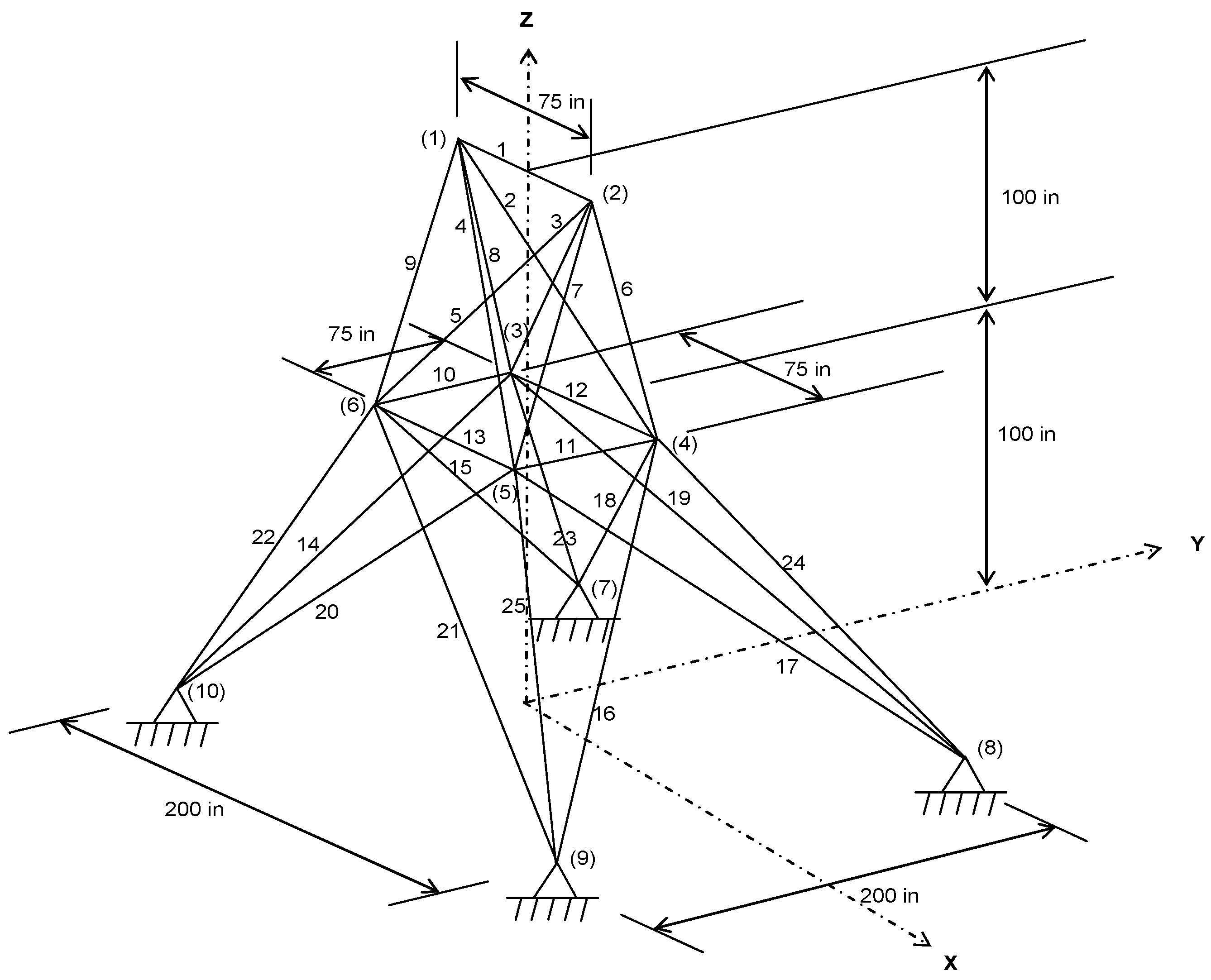
4.2. Spatial 25-Bar Truss Structure
The second test problem regards the spatial 25-bar truss shown in Figure 4. The modulus of elasticity and material density are the same as in the previous test case. The 25 truss members are organized into 8 groups, as follows: (1) A1, (2) A2–A5, (3) A6–A9, (4) A10–A11, (5) A12–A13, (6) A14–A17, (7) A18–A21, and (8) A22–A25. The cross-sectional areas of the bars are defined as the design variables and vary between 0.01 inch2 and 3.5 inch2. The weight of the structure is minimized, subject to all members satisfying the stress limits in Table 3 and nodal displacement limits in three directions of ±0.35 inch. There is a total of 110 inequality constraints. The truss is subject to the two independent loading conditions listed in Table 4, where , and are the loads along x-, y- and z-axis, respectively.
This truss problem has been previously studied by using deterministic global methods [3] and many stochastic optimization methods [21,27,28,31,34,35,36,37,38,39,41,45]. Table 5 compares the best designs found by ALSSO and the above-mentioned stochastic methods. Among the deterministic global methods, the Pareto–Lipschitzian Optimization with Reduced-set (PLOR) algorithm is better than the three DIRECT-type algorithms [3]. Therefore, only the optimized result obtained by PLOR is listed in Table 5. All the published results satisfy the limits on the stress. To the best of our knowledge, CA [37] generated the best design for this test problem. The best designs from HM, HPSSO, improved TLBO, FPA, and WEO slightly violated the nodal displacement constraints. It can be seen from Table 5 that the proposed algorithm produced better designs than PLOR, HS, HPSO, SSO ABC-AP, SAHB, and MSPSO, and comparable with TLBO.
Statistical data listed in Table 6 prove that the present algorithm was also very robust for this test problem.
Figure 5 shows the convergence curve obtained for the last optimization run with N = 500. For both load cases, ALSSO detected the y-displacement constraints of top nodes as active.
4.3. Spatial 72-Bar Truss Structure
The third test example regards the optimal design of the spatial 72-bar truss structure shown in Figure 6. The modulus of elasticity and material density are the same as in the previous test cases. The 72 members are organized into 16 groups, as follows: (1) A1–A4, (2) A5–A12, (3) A13–A16, (4) A17–A18, (5) A19–A22, (6) A23–A30, (7) A31–A34, (8) A35–A36, (9) A37–A40, (10) A41–A48, (11) A49–A52, (12) A53–A54, (13) A55–A58, (14) A59–A66, (15) A67–A70, and (16) A71–A72. The truss structure is subject to 160 constraints on stress and displacement. A displacement limit within ±0.25 inch is imposed on the top nodes in both x and y directions, and all truss elements have an axial stress limit within ±25 ksi. The truss is subject to the two independent loading conditions listed in Table 7.
This truss problem has been previously studied using deterministic global methods [3], a GA-based method [9], HS [28], ACO [16], PSO [23], ALPSO [25], BB-BC [33], SAHS [27], TLBO [34], CA [37], and WEO [39]. Their best designs are compared against that obtained by the proposed method, and are shown in Table 8. The proposed method produced a new best design with a weight of 379.5922 lb. Among the deterministic global methods, the DIRECT-l algorithm found the best design for this test case (Table 8). However, the corresponding structural weight is larger than the structural weight obtained by the proposed method. It should be noted that the maximum displacements of GA, HS, ALPSO, BB-BC, and FPA exceed the x- and y-displacement limits on node 17. In particular, the optimum design found by HS also violates the compressive stress limits of bar members 55, 56, 57, and 58 under load case 2. The optimum design found by the proposed method satisfies both stress limits and displacement limits and is better than SAHS, TLBO, and CA.
Statistical data listed in Table 9 prove that the present algorithm was also very robust for this test problem.
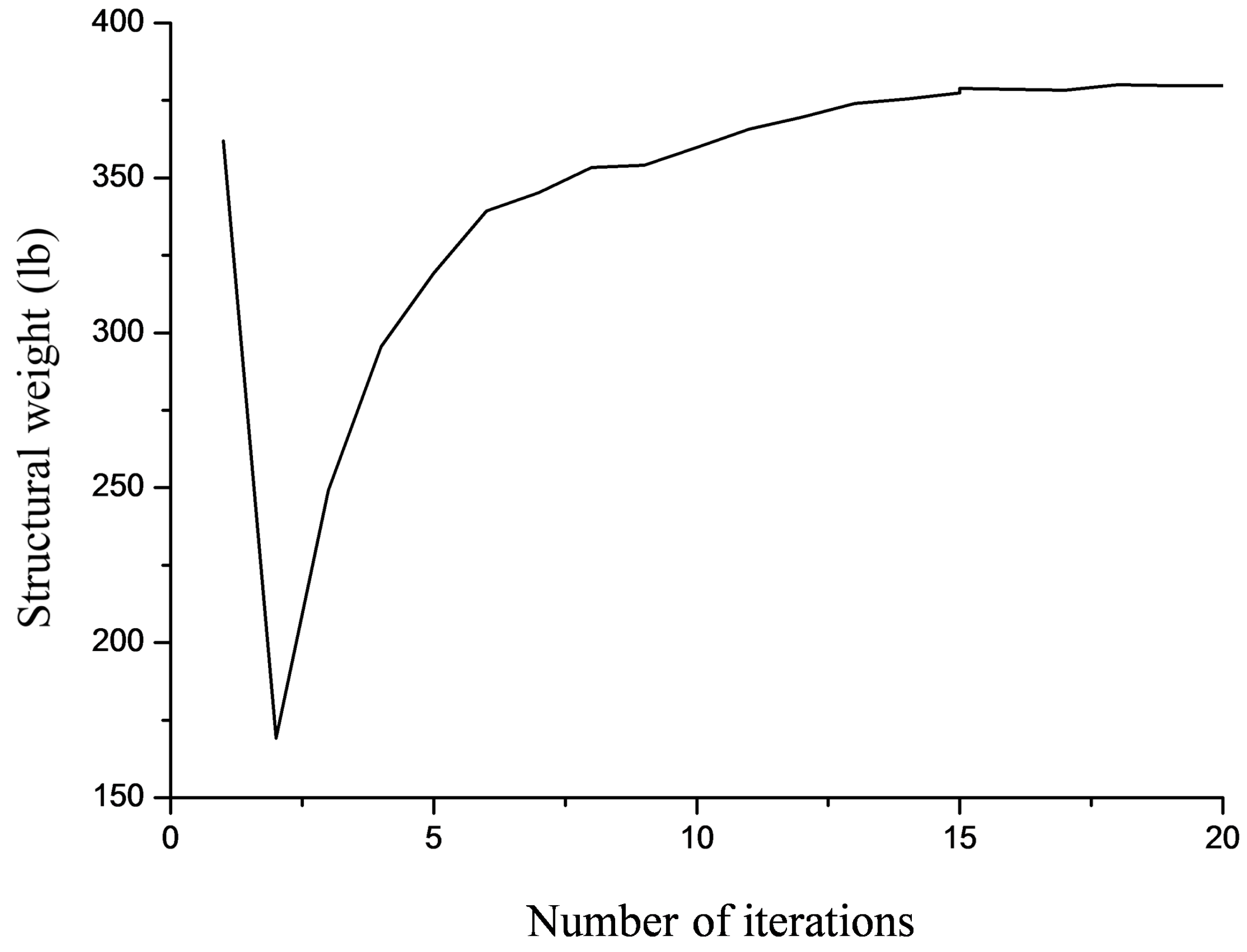
Figure 7 shows the convergence curve obtained for the last optimization run with N = 500. ALSSO detected the x- and y-displacement constraints of node 17 for load case 1 as active.
4.4. Planar 200-Bar Truss Structure
The last test example regards the optimal design of the planar 200-bar truss structure shown in Figure 8. The modulus of elasticity is 30 Msi and the mass density is 0.283 lb/inch3. The stress limit on all elements is ±10 ksi. There are no displacement constraints. The structural elements are divided into 29 groups as shown in Figure 8. The minimum cross-sectional area of all design variables is 0.1 inch2. The structure is designed against three independent loading conditions: (1) 1.0 kip acting in the positive x-direction at nodes 1, 6, 15, 20, 29, 34, 43, 48, 57, 62, and 71; (2) 10.0 kips acting in the negative y-direction at nodes 1, 2, 3, 4, 5, 6, 8, 10, 12, 14, 15, 16, 17, 18, 19, 20, 22, 24, 26, 28, 29,30, 31, 32, 33, 34, 36, 38, 40, 42, 43, 44, 45, 46, 47, 48, 50, 52, 54, 56, 57, 58, 59, 60, 61, 62, 64, 66, 68, 70, 71, 72, 73, 74, and 75; (3) loading conditions (1) and (2) acting together.
This truss problem has been previously studied using SAHS [27], TLBO [34], ABC-AP [36], WEO [39], FPA [38], HPSACO [40], and HPSSO [41]. The optimized designs are compared in Table 10. SAHS, TLBO, HPSSO, and WEO generated feasible designs while HPSACO, ABC-AP, FPA, and ALSSO slightly violated the constraints. TLBO produced the best design for this test problem.
5. Conclusions
This paper presented a hybrid algorithm for structural optimization, named ALSSO, which combines subset simulation optimization (SSO) with the dynamic augmented Lagrangian multiplier method (DALMM). The performance of SSO is comparable to other stochastic optimization methods. ALSSO employs DALMM to decompose the original constrained problem into a series of unconstrained optimization sub-problems, and uses SSO to solve each unconstrained optimization sub-problem. By adaptively updating the Lagrangian multipliers and penalty parameters, the proposed method can automatically detect active constraints and provide the globally optimal solution to the problem at hand.
Four classical truss sizing problems were used to verify the accuracy and robustness of ALSSO. Compared to the results published in the literature, it is found that the proposed method is able to produce equivalent solutions. It also shows a remarkable statistical performance based on 30 independent runs. A potential drawback of ALSSO at present is that its convergence rate will slow down when the search process approaches the active constraints. In the future, we will introduce a local search strategy into ALSSO to further improve its efficiency and apply ALSSO to various real-life problems.
Acknowledgments
The authors are grateful for the supports by the Natural Science Foundation of China (Grant No. U1533109).
Author Contributions
Feng Du and Hong-Shuang Li conceived, designed and coded the algorithm; Qiao-Yue Dong computed and analyzed the first three examples; Feng Du computed and analyzed the forth example; Feng Du and Hong-Shuang Li wrote the paper.
Conflicts of Interest
The authors declare no conflict of interest.
References
- Haftka, R.; Gurdal, Z. Elements of Structural Optimization, 3th ed.; Kluwer Academic Publishers: Dordrecht, The Netherlands, 1992. [Google Scholar]
- Jones, D.R.; Perttunen, C.D.; Stuckman, B.E. Lipschitzian optimization without the Lipschitz constant. J. Opt. Theory Appl. 1993, 79, 157–181. [Google Scholar] [CrossRef]
- Mockus, J.; Paulavičius, R.; Rusakevičius, D.; Šešok, D.; Žilinskas, J. Application of Reduced-set Pareto-Lipschitzian Optimization to truss optimization. J. Glob. Opt. 2017, 67, 425–450. [Google Scholar] [CrossRef]
- Kvasov, D.E.; Sergeyev, Y.D. Deterministic approaches for solving practical black-box global optimization problems. Adv. Eng. Softw. 2015, 80 (Suppl. C), 58–66. [Google Scholar] [CrossRef]
- Kvasov, D.E.; Mukhametzhanov, M.S. Metaheuristic vs. deterministic global optimization algorithms: The univariate case. Appl. Math. Comput. 2018, 318, 245–259. [Google Scholar] [CrossRef]
- Adeli, H.; Kumar, S. Distributed genetic algorithm for structural optimization. J. Aerosp. Eng. 1995, 8, 156–163. [Google Scholar] [CrossRef]
- Kameshki, E.S.; Saka, M.P. Optimum geometry design of nonlinear braced domes using genetic algorithm. Comput. Struct. 2007, 85, 71–79. [Google Scholar] [CrossRef]
- Rajeev, S.; Krishnamoorthy, C.S. Discrete optimization of structures using genetic algorithms. J. Struct. Eng. 1992, 118, 1233–1250. [Google Scholar] [CrossRef]
- Wu, S.J.; Chow, P.T. Steady-state genetic algorithms for discrete optimization of trusses. Comput. Struct. 1995, 56, 979–991. [Google Scholar] [CrossRef]
- Saka, M.P. Optimum design of pitched roof steel frames with haunched rafters by genetic algorithm. Comput. Struct. 2003, 81, 1967–1978. [Google Scholar] [CrossRef]
- Erbatur, F.; Hasançebi, O.; Tütüncü, İ.; Kılıç, H. Optimal design of planar and space structures with genetic algorithms. Comput. Struct. 2000, 75, 209–224. [Google Scholar] [CrossRef]
- Galante, M. Structures optimization by a simple genetic algorithm. In Numerical Methods in Engineering and Applied Sciences; Centro Internacional de Métodos Numéricos en Ingeniería: Barcelona, Spain, 1992; pp. 862–870. [Google Scholar]
- Bennage, W.A.; Dhingra, A.K. Single and multiobjective structural optimization in discrete-continuous variables using simulated annealing. Int. J. Numer. Methods Eng. 1995, 38, 2753–2773. [Google Scholar] [CrossRef]
- Lamberti, L. An efficient simulated annealing algorithm for design optimization of truss structures. Comput. Struct. 2008, 86, 1936–1953. [Google Scholar] [CrossRef]
- Leite, J.P.B.; Topping, B.H.V. Parallel simulated annealing for structural optimization. Comput. Struct. 1999, 73, 545–564. [Google Scholar] [CrossRef]
- Camp, C.V.; Bichon, B.J. Design of Space Trusses Using Ant Colony Optimization. J. Struct. Eng. 2004, 130, 741–751. [Google Scholar] [CrossRef]
- Kaveh, A.; Talatahari, S. A particle swarm ant colony optimization for truss structures with discrete variables. J. Constr. Steel Res. 2009, 65, 1558–1568. [Google Scholar] [CrossRef]
- Kaveh, A.; Shojaee, S. Optimal design of skeletal structures using ant colony optimisation. Int. J. Numer. Methods Eng. 2007, 70, 563–581. [Google Scholar] [CrossRef]
- Kaveh, A.; Farahmand Azar, B.; Talatahari, S. Ant colony optimization for design of space trusses. Int. J. Space Struct. 2008, 23, 167–181. [Google Scholar] [CrossRef]
- Li, L.J.; Huang, Z.B.; Liu, F. A heuristic particle swarm optimization method for truss structures with discrete variables. Comput. Struct. 2009, 87, 435–443. [Google Scholar] [CrossRef]
- Li, L.J.; Huang, Z.B.; Liu, F.; Wu, Q.H. A heuristic particle swarm optimizer for optimization of pin connected structures. Comput. Struct. 2007, 85, 340–349. [Google Scholar] [CrossRef]
- Luh, G.C.; Lin, C.Y. Optimal design of truss-structures using particle swarm optimization. Comput. Struct. 2011, 89, 2221–2232. [Google Scholar] [CrossRef]
- Perez, R.E.; Behdinan, K. Particle swarm approach for structural design optimization. Comput. Struct. 2007, 85, 1579–1588. [Google Scholar] [CrossRef]
- Dong, Y.; Tang, J.; Xu, B.; Wang, D. An application of swarm optimization to nonlinear programming. Comput. Math. Appl. 2005, 49, 1655–1668. [Google Scholar] [CrossRef]
- Jansen, P.W.; Perez, R.E. Constrained structural design optimization via a parallel augmented Lagrangian particle swarm optimization approach. Comput. Struct. 2011, 89, 1352–1366. [Google Scholar] [CrossRef]
- Sedlaczek, K.; Eberhard, P. Using augmented Lagrangian particle swarm optimization for constrained problems in engineering. Struct. Multidiscip. Opt. 2006, 32, 277–286. [Google Scholar] [CrossRef]
- Talatahari, S.; Kheirollahi, M.; Farahmandpour, C.; Gandomi, A.H. A multi-stage particle swarm for optimum design of truss structures. Neural Comput. Appl. 2013, 23, 1297–1309. [Google Scholar] [CrossRef]
- Lee, K.S.; Geem, Z.W. A new structural optimization method based on the harmony search algorithm. Comput. Struct. 2004, 82, 781–798. [Google Scholar] [CrossRef]
- Lee, K.S.; Geem, Z.W.; Lee, S.H.; Bae, K.W. The harmony search heuristic algorithm for discrete structural optimization. Eng. Opt. 2005, 37, 663–684. [Google Scholar] [CrossRef]
- Saka, M. Optimum geometry design of geodesic domes using harmony search algorithm. Adv. Struct. Eng. 2007, 10, 595–606. [Google Scholar] [CrossRef]
- Degertekin, S.O. Improved harmony search algorithms for sizing optimization of truss structures. Comput. Struct. 2012, 92 (Suppl. C), 229–241. [Google Scholar] [CrossRef]
- Kaveh, A.; Talatahari, S. Optimal design of skeletal structures via the charged system search algorithm. Struct. Multidiscip. Opt. 2010, 41, 893–911. [Google Scholar] [CrossRef]
- Kaveh, A.; Talatahari, S. Size optimization of space trusses using Big Bang–Big Crunch algorithm. Comput. Struct. 2009, 87, 1129–1140. [Google Scholar] [CrossRef]
- Degertekin, S.O.; Hayalioglu, M.S. Sizing truss structures using teaching-learning-based optimization. Comput. Struct. 2013, 119 (Suppl. C), 177–188. [Google Scholar] [CrossRef]
- Camp, C.V.; Farshchin, M. Design of space trusses using modified teaching–learning based optimization. Eng. Struct. 2014, 62 (Suppl. C), 87–97. [Google Scholar] [CrossRef]
- Sonmez, M. Artificial Bee Colony algorithm for optimization of truss structures. Appl. Soft Comput. 2011, 11, 2406–2418. [Google Scholar] [CrossRef]
- Jalili, S.; Hosseinzadeh, Y. A Cultural Algorithm for Optimal Design of Truss Structures. Latin Am. J. Solids Struct. 2015, 12, 1721–1747. [Google Scholar] [CrossRef]
- Bekdaş, G.; Nigdeli, S.M.; Yang, X.-S. Sizing optimization of truss structures using flower pollination algorithm. Appl. Soft Comput. 2015, 37 (Suppl. C), 322–331. [Google Scholar] [CrossRef]
- Kaveh, A.; Bakhshpoori, T. A new metaheuristic for continuous structural optimization: Water evaporation optimization. Struct. Multidiscip. Opt. 2016, 54, 23–43. [Google Scholar] [CrossRef]
- Kaveh, A.; Talatahari, S. Particle swarm optimizer, ant colony strategy and harmony search scheme hybridized for optimization of truss structures. Comput. Struct. 2009, 87, 267–283. [Google Scholar] [CrossRef]
- Kaveh, A.; Bakhshpoori, T.; Afshari, E. An efficient hybrid Particle Swarm and Swallow Swarm Optimization algorithm. Comput. Struct. 2014, 143, 40–59. [Google Scholar] [CrossRef]
- Lamberti, L.; Pappalettere, C. Metaheuristic Design Optimization of Skeletal Structures: A Review. Comput. Technol. Rev. 2011, 4, 1–32. [Google Scholar] [CrossRef]
- Bertsekas, D.P. Constrained Optimization and Lagrange Multiplier Methods; Athena Scientific: Belmont, TN, USA, 1996. [Google Scholar]
- Li, H.S. Subset simulation for unconstrained global optimization. Appl. Math. Model. 2011, 35, 5108–5120. [Google Scholar] [CrossRef]
- Li, H.S.; Au, S.K. Design optimization using Subset Simulation algorithm. Struct. Saf. 2010, 32, 384–392. [Google Scholar] [CrossRef]
- Li, H.S.; Ma, Y.Z. Discrete optimum design for truss structures by subset simulation algorithm. J. Aerosp. Eng. 2015, 28, 04014091. [Google Scholar] [CrossRef]
- Au, S.K.; Ching, J.; Beck, J.L. Application of subset simulation methods to reliability benchmark problems. Struct. Saf. 2007, 29, 183–193. [Google Scholar] [CrossRef]
- Au, S.K.; Beck, J.L. Estimation of small failure probabilities in high dimensions by subset simulation. Probab. Eng. Mech. 2001, 16, 263–277. [Google Scholar] [CrossRef]
- Coello, C.A.C. Theoretical and numerical constraint-handling techniques used with evolutionary algorithms: A survey of the state of the art. Comput. Methods Appl. Mech. Eng. 2002, 191, 1245–1287. [Google Scholar] [CrossRef]
- Long, W.; Liang, X.; Huang, Y.; Chen, Y. A hybrid differential evolution augmented Lagrangian method for constrained numerical and engineering optimization. Comput.-Aided Des. 2013, 45, 1562–1574. [Google Scholar] [CrossRef]
- Au, S.K. Reliability-based design sensitivity by efficient simulation. Comput. Struct. 2005, 83, 1048–1061. [Google Scholar] [CrossRef]
Figure 1.
Flowchart of the proposed method.
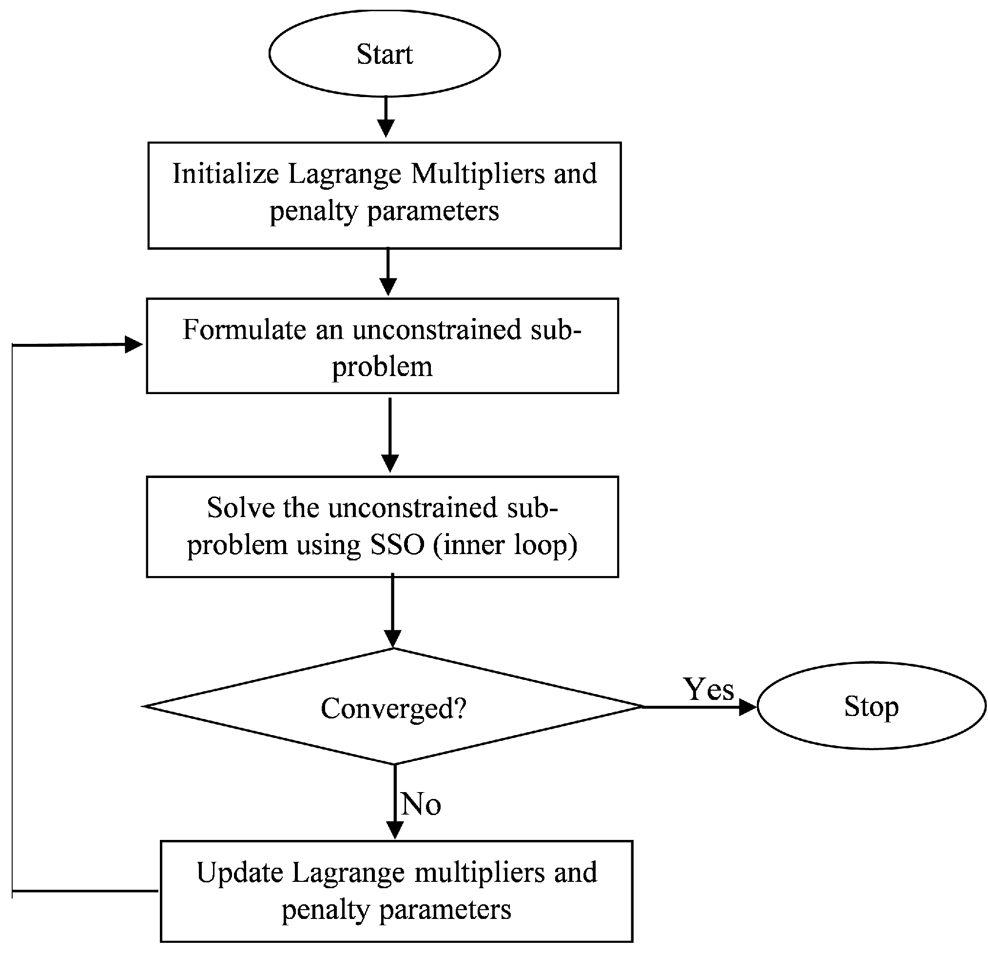
Figure 2.
Schematic of the planar 10-bar truss structure.
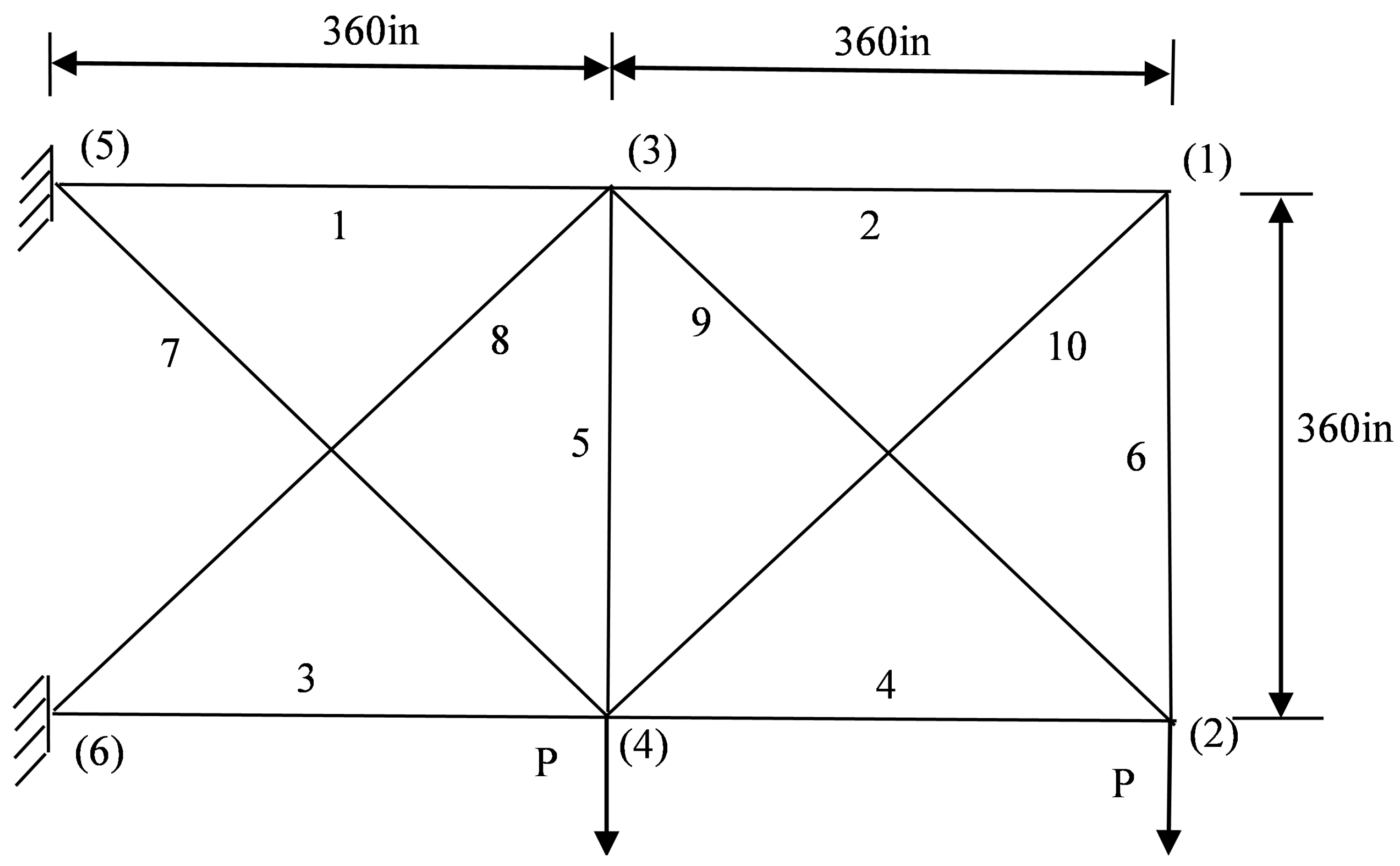
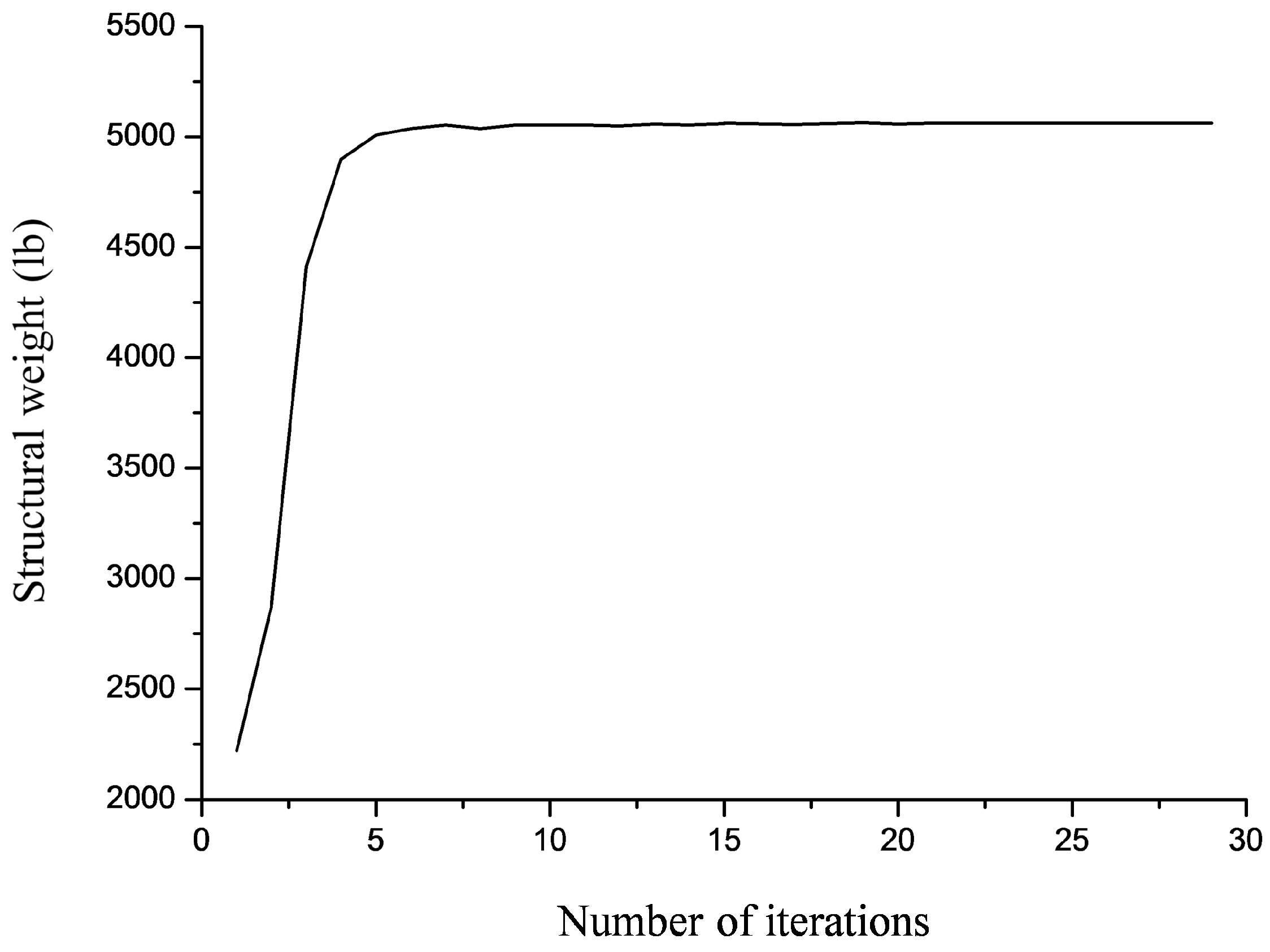
Figure 3.
Convergence curve obtained for the 10-bar truss problem with N = 500.

Figure 4.
Schematic of the spatial 25-bar truss structure.

Figure 5.
Convergence curve obtained for the 25-bar truss problem with N = 500.
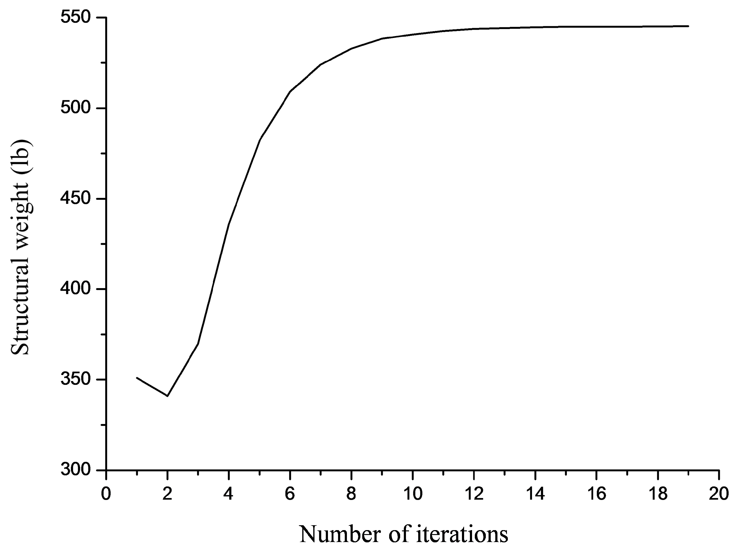
Figure 6.
Schematic of the spatial 72-bar truss structure.
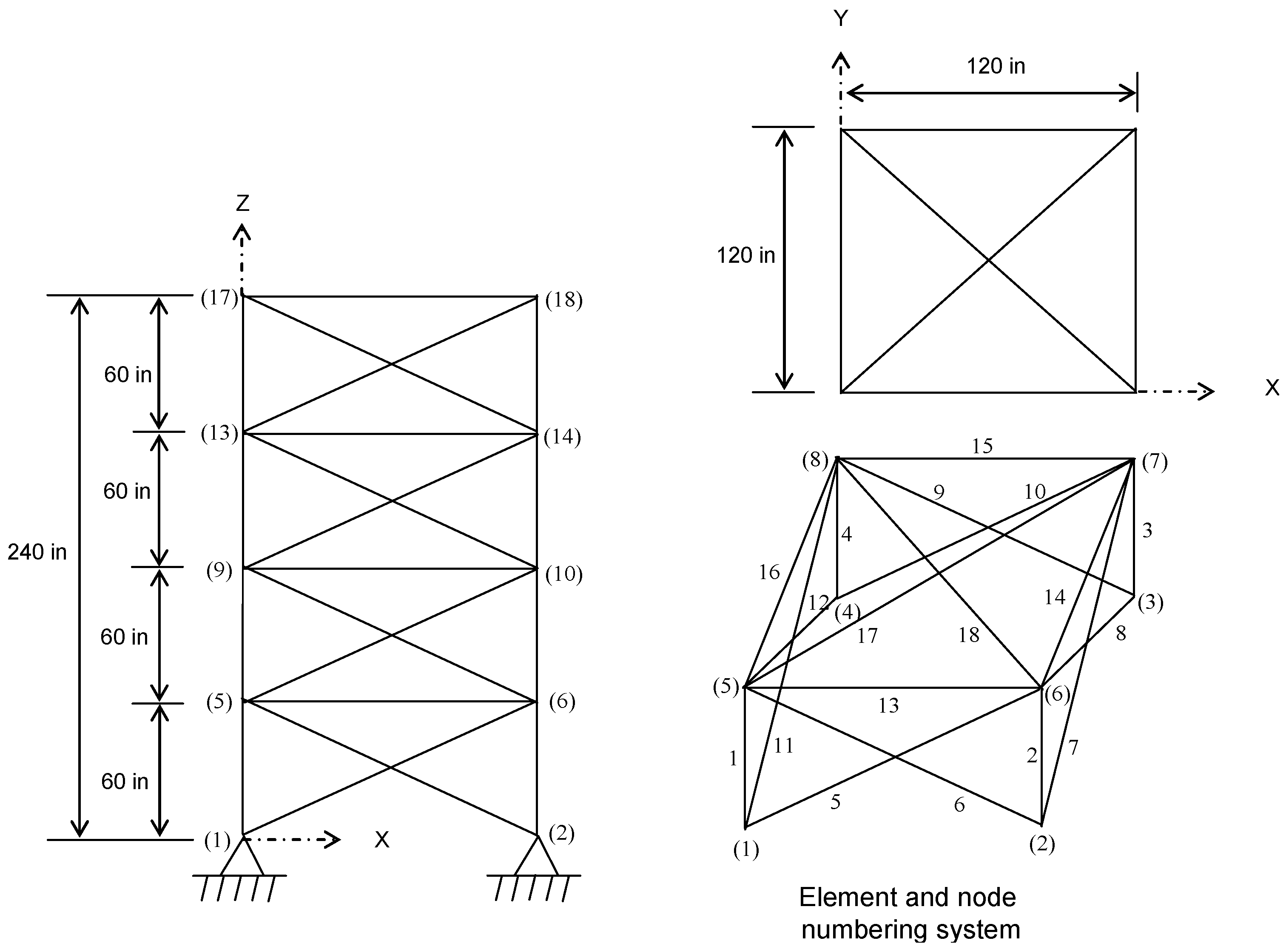
Figure 7.
Convergence curve obtained for the 72-bar truss problem with N = 500.

Figure 8.
Schematic of the planar 200-bar truss structure.
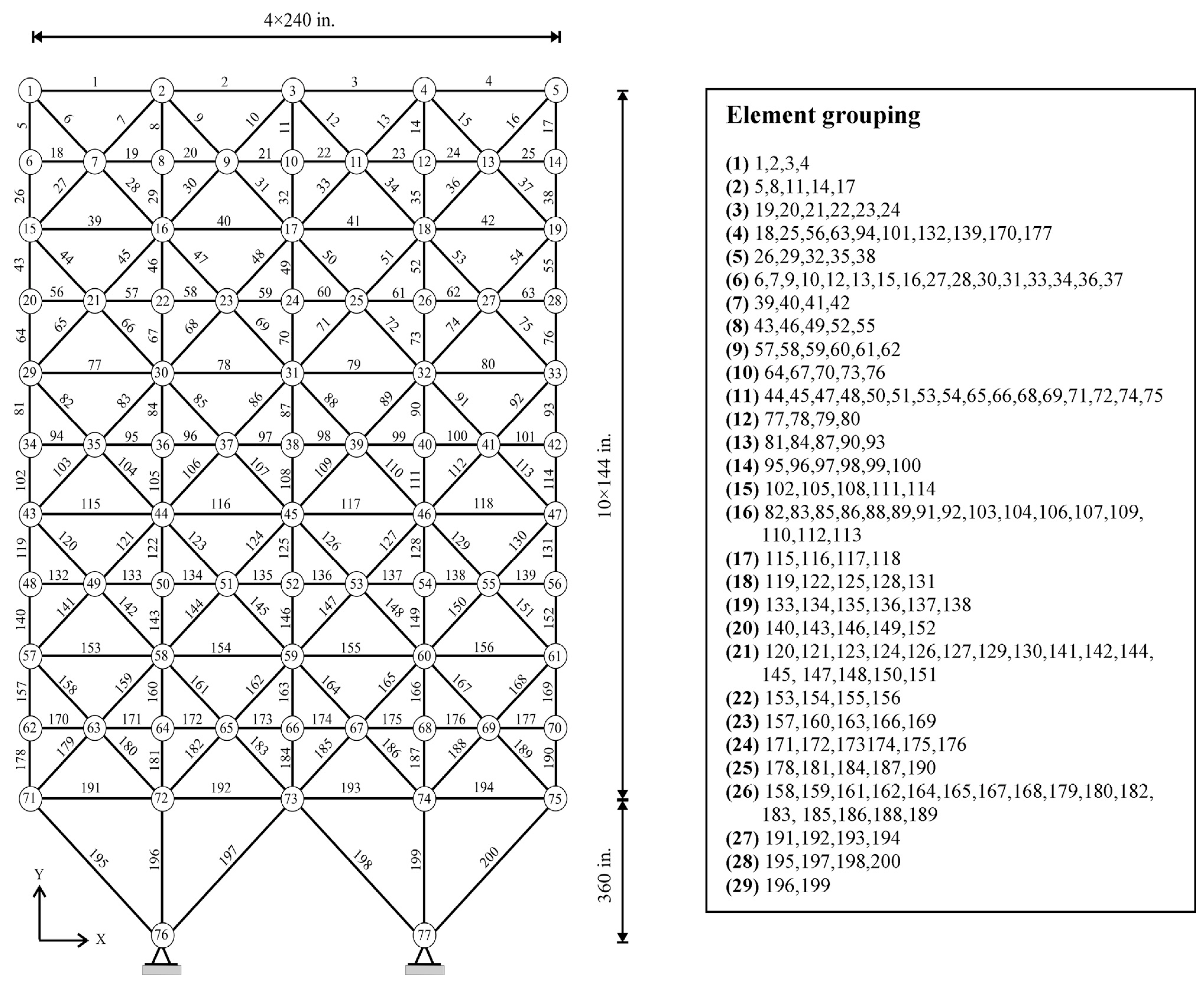
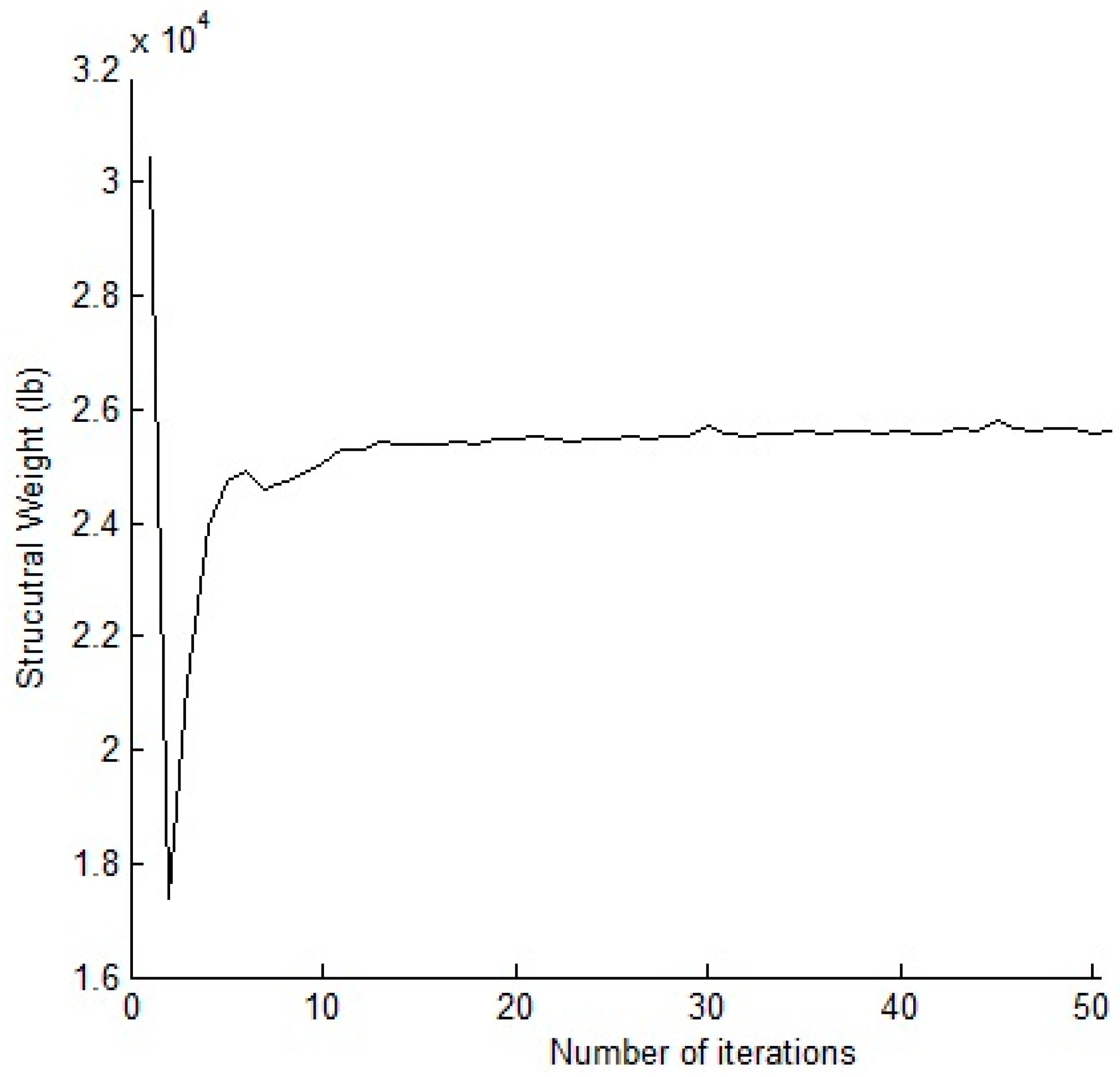
Figure 9.
Convergence curve obtained for the 200-bar truss problem with N = 500.

Table 1.
Comparison of optimized designs for the 10-bar truss problem.
| Design Variables | GA [12] | HPSO [21] | HS [28] | HPSACO [17] | PSO [23] | ALPSO [25] | HPSACO [40] | ABC-AP [36] | SAHS [31] | TLBO [34] | MSPSO [27] | HPSSO [41] | WEO [39] | ALSSO |
|---|---|---|---|---|---|---|---|---|---|---|---|---|---|---|
| A1 | 30.440 | 30.704 | 30.150 | 30.493 | 33.500 | 30.511 | 30.307 | 30.548 | 30.394 | 30.4286 | 30.5257 | 30.5838 | 30.5755 | 30.4397 |
| A2 | 0.100 | 0.100 | 0.102 | 0.100 | 0.100 | 0.100 | 0.1 | 0.1 | 0.1 | 0.1 | 0.1001 | 0.1 | 0.1 | 0.1004 |
| A3 | 21.790 | 23.167 | 22.710 | 23.230 | 22.766 | 23.230 | 23.434 | 23.18 | 23.098 | 23.2436 | 23.225 | 23.15103 | 23.3368 | 23.1599 |
| A4 | 14.260 | 15.183 | 15.270 | 15.346 | 14.417 | 15.198 | 15.505 | 15.218 | 15.491 | 15.3677 | 15.4114 | 15.20566 | 15.1497 | 15.2446 |
| A5 | 0.100 | 0.100 | 0.102 | 0.100 | 0.100 | 0.100 | 0.1 | 0.1 | 0.1 | 0.1 | 0.1001 | 0.1 | 0.1 | 0.1003 |
| A6 | 0.451 | 0.551 | 0.544 | 0.538 | 0.100 | 0.554 | 0.5241 | 0.551 | 0.529 | 0.5751 | 0.5583 | 0.548897 | 0.5276 | 0.5455 |
| A7 | 21.630 | 20.978 | 21.560 | 20.990 | 20.392 | 21.017 | 21.079 | 21.058 | 21.189 | 20.9665 | 20.9172 | 21.06437 | 20.9892 | 21.1123 |
| A8 | 7.628 | 7.460 | 7.541 | 7.451 | 7.534 | 7.452 | 7.4365 | 7.463 | 7.488 | 7.4404 | 7.4395 | 7.465322 | 7.4458 | 7.4660 |
| A9 | 0.100 | 0.100 | 0.100 | 0.100 | 0.100 | 0.100 | 0.1 | 0.1 | 0.1 | 0.1 | 0.1 | 0.1 | 0.1 | 0.1000 |
| A10 | 21.360 | 21.508 | 21.458 | 21.458 | 20.467 | 21.554 | 21.229 | 21.501 | 21.342 | 21.533 | 21.5098 | 21.52935 | 21.5236 | 21.5191 |
| Weight (lb) | 4987.00 | 5060.92 | 5057.88 | 5058.43 | 5024.25 | 5060.85 | 5056.56 | 5060.88 | 5061.42 | 5060.96 | 5061.00 | 5060.86 | 5060.99 | 5060.885 |
Table 2.
Comparison of statistical performance in the 10-bar truss problem.
| Method | N | Best | Mean | Worst | SD | NSA |
|---|---|---|---|---|---|---|
| ALSSO | 100 | 5060.931 | 5064.559 | 5079.894 | 3.363699 | 48,064 (44,710) |
| 200 | 5060.931 | 5062.391 | 5065.715 | 0.889472 | 94,540 (108,600) | |
| 500 | 5060.885 | 5061.713 | 5062.291 | 0.360457 | 247,828 (253,400) | |
| HPSACO [33] | 5056.56 | 5057.66 | 5061.12 | 1.42 | 10,650 | |
| ABC-AP [36] | 5060.88 | N/A | 5060.95 | N/A | 500,000 | |
| SAHS [31] | 5061.42 | 5061.95 | 5063.39 | 0.71 | 7081 | |
| TLBO [34] | 5060.96 | 5062.08 | 5063.23 | 0.79 | 16,872 | |
| MSPSO [27] | 5061.00 | 5064.46 | 5078.00 | 5.72 | N/A | |
| HPSSO [41] | 5060.86 | 5062.28 | 5076.90 | 4.325 | 14,118 | |
| WEO [39] | 5060.99 | 5062.09 | 5975.41 | 2.05 | 19,540 |
Table 3.
Stress limits for the 25-bar truss problem.
| Design Variables | Compressive Stress Limit (ksi) | Tensile Stress Limit (ksi) | |
|---|---|---|---|
| 1 | A1 | 35.092 | 40.0 |
| 2 | A2–A5 | 11.590 | 40.0 |
| 3 | A6–A9 | 17.305 | 40.0 |
| 4 | A10–A11 | 35.092 | 40.0 |
| 5 | A12–A13 | 35.092 | 40.0 |
| 6 | A14–A17 | 6.759 | 40.0 |
| 7 | A18–A21 | 6.957 | 40.0 |
| 8 | A22–A25 | 11.802 | 40.0 |
Table 4.
Loading conditions acting on the 25-bar truss.
| Load Cases | Nodes | Loads | ||
|---|---|---|---|---|
| Px (kips) | Py (kips) | Pz (kips) | ||
| 1 | 1 | 0.0 | 20.0 | −5.0 |
| 2 | 0.0 | −20.0 | −5.0 | |
| 2 | 1 | 1.0 | 10.0 | −5.0 |
| 2 | 0.0 | 10.0 | −5.0 | |
| 3 | 0.5 | 0.0 | 0.0 | |
| 6 | 0.5 | 0.0 | 0.0 | |
Table 5.
Comparison of optimized designs for the 25-bar truss problem.
| Design Variables | HS [28] | HPSO [21] | SSO [45] | PLOR [3] | ABC-AP [36] | SAHS [31] | TLBO [34] | MSPSO [27] | CA [37] | HPSSO [41] | TLBO [35] | FPA [38] | WEO [39] | ALSSO | |
|---|---|---|---|---|---|---|---|---|---|---|---|---|---|---|---|
| 1 | A1 | 0.047 | 0.010 | 0.010 | 0.010 | 0.011 | 0.01 | 0.01 | 0.01 | 0.01 | 0.01 | 0.01 | 0.01 | 0.01 | 0.01001 |
| 2 | A2–A5 | 2.022 | 1.970 | 2.057 | 1.951 | 1.979 | 2.074 | 2.0712 | 1.9848 | 2.02064 | 1.9907 | 1.9878 | 1.8308 | 1.9184 | 1.983579 |
| 3 | A6–A9 | 2.950 | 3.016 | 2.892 | 3.025 | 3.003 | 2.961 | 2.957 | 2.9956 | 3.01733 | 2.9881 | 2.9914 | 3.1834 | 3.0023 | 2.998787 |
| 4 | A10–A11 | 0.010 | 0.010 | 0.010 | 0.010 | 0.01 | 0.01 | 0.01 | 0.01 | 0.01 | 0.01 | 0.0102 | 0.01 | 0.01 | 0.010008 |
| 5 | A12–A13 | 0.014 | 0.010 | 0.014 | 0.010 | 0.01 | 0.01 | 0.01 | 0.01 | 0.01 | 0.01 | 0.01 | 0.01 | 0.01 | 0.010005 |
| 6 | A14–A17 | 0.688 | 0.694 | 0.697 | 0.592 | 0.69 | 0.691 | 0.6891 | 0.6852 | 0.69383 | 0.6824 | 0.6828 | 0.7017 | 0.6827 | 0.683045 |
| 7 | A18–A21 | 1.657 | 1.681 | 1.666 | 1.706 | 1.679 | 1.617 | 1.6209 | 1.6778 | 1.63422 | 1.6764 | 1.6775 | 1.7266 | 1.6778 | 1.677394 |
| 8 | A22–A25 | 2.663 | 2.643 | 2.675 | 2.789 | 2.652 | 2.674 | 2.6768 | 2.6599 | 2.65277 | 2.6656 | 2.664 | 2.5713 | 2.6612 | 2.66077 |
| Weight (lb) | 544.38 | 545.19 | 545.37 | 546.80 | 545.193 | 545.12 | 545.09 | 545.172 | 545.05 | 545.164 | 545.175 | 545.159 | 545.166 | 545.1057 | |
Table 6.
Comparison of statistical performance in the 25-bar truss problem.
| N | Best | Mean | Worst | SD | NSA | |
|---|---|---|---|---|---|---|
| ALSSO | 100 | 545.1241 | 545.2569 | 545.7793 | 0.135161 | 27,009 (23,170) |
| 200 | 545.1254 | 545.205 | 545.4292 | 0.067821 | 38,301 (32,580) | |
| 500 | 545.1057 | 545.185 | 545.2819 | 0.044924 | 86,490 (90,500) | |
| ABC-AP [36] | 545.19 | N/A | 545.28 | N/A | 300,000 | |
| SAHS [31] | 545.12 | 545.94 | 546.6 | 0.91 | 9051 | |
| TLBO [34] | 545.09 | 545.41 | 546.33 | 0.42 | 15,318 | |
| MSPSO [27] | 545.172 | 546.03 | 548.78 | 0.8 | 10,800 | |
| CA [37] | 545.05 | 545.93 | N/A | 1.55 | 9380 | |
| HPSSO [41] | 545.164 | 545.556 | 546.99 | 0.432 | 13,326 | |
| TLBO [35] | 545.175 | 545.483 | N/A | 0.306 | 12,199 | |
| FPA [38] | 545.159 | 545.73 | N/A | 0.59 | 8149 | |
| WEO [39] | 545.166 | 545.226 | 545.592 | 0.083 | 19,750 |
Table 7.
Loading conditions acting on the 72-bar truss.
| Node | Case 1 (kips) | Case 2 (kips) | ||||
|---|---|---|---|---|---|---|
| Px | Py | Pz | Px | Py | Pz | |
| 17 | 5.0 | 5.0 | −5.0 | 0.0 | 0.0 | −5.0 |
| 18 | 0.0 | 0.0 | 0.0 | 0.0 | 0.0 | −5.0 |
| 19 | 0.0 | 0.0 | 0.0 | 0.0 | 0.0 | −5.0 |
| 20 | 0.0 | 0.0 | 0.0 | 0.0 | 0.0 | −5.0 |
Table 8.
Comparison of optimized designs for the 72-bar truss problem.
| Design Variables | GA [11] | ACO [16] | HS [28] | PSO [23] | ALPSO [25] | DIRECT-l [3] | BB-BC [33] | SAHS [27] | TLBO [34] | CA [37] | FPA [38] | ALSSO |
|---|---|---|---|---|---|---|---|---|---|---|---|---|
| A1–A4 | 1.910 | 1.948 | 1.790 | 1.743 | 1.898 | 1.699 | 1.9042 | 1.86 | 1.8807 | 1.86093 | 1.8758 | 1.900283 |
| A5–A12 | 0.525 | 0.508 | 0.521 | 0.519 | 0.513 | 0.476 | 0.5162 | 0.521 | 0.5142 | 0.5093 | 0.516 | 0.511187 |
| A13–A16 | 0.122 | 0.101 | 0.100 | 0.100 | 0.100 | 0.100 | 0.1 | 0.1 | 0.1 | 0.1 | 0.1 | 0.100084 |
| A17–A18 | 0.103 | 0.102 | 0.100 | 0.100 | 0.100 | 0.100 | 0.1 | 0.1 | 0.1 | 0.1 | 0.1 | 0.100258 |
| A19–A22 | 1.310 | 1.303 | 1.229 | 1.308 | 1.258 | 1.371 | 1.2582 | 1.293 | 1.2711 | 1.26291 | 1.2993 | 1.268814 |
| A23–A30 | 0.498 | 0.511 | 0.522 | 0.519 | 0.513 | 0.547 | 0.5035 | 0.511 | 0.5151 | 0.50397 | 0.5246 | 0.510226 |
| A31–A34 | 0.100 | 0.101 | 0.100 | 0.100 | 0.100 | 0.100 | 0.1 | 0.1 | 0.1 | 0.1 | 0.1001 | 0.100076 |
| A35–A36 | 0.103 | 0.100 | 0.100 | 0.100 | 0.100 | 0.100 | 0.1 | 0.1 | 0.1 | 0.1 | 0.1 | 0.100113 |
| A37–A40 | 0.535 | 0.561 | 0.517 | 0.514 | 0.520 | 0.618 | 0.5178 | 0.499 | 0.5317 | 0.52316 | 0.4971 | 0.519311 |
| A41–A48 | 0.535 | 0.492 | 0.504 | 0.546 | 0.518 | 0.476 | 0.5214 | 0.501 | 0.5134 | 0.52522 | 0.5089 | 0.516303 |
| A49–A52 | 0.103 | 0.100 | 0.100 | 0.100 | 0.100 | 0.100 | 0.1 | 0.1 | 0.1 | 0.10001 | 0.1 | 0.100062 |
| A53–A54 | 0.111 | 0.107 | 0.101 | 0.110 | 0.100 | 0.112 | 0.1007 | 0.1 | 0.1 | 0.10254 | 0.1 | 0.100502 |
| A55–A58 | 0.161 | 0.156 | 0.156 | 0.162 | 0.157 | 0.153 | 0.1566 | 0.168 | 0.1565 | 0.155962 | 0.1575 | 0.156389 |
| A59–A66 | 0.544 | 0.550 | 0.547 | 0.509 | 0.546 | 0.582 | 0.5421 | 0.584 | 0.5429 | 0.55349 | 0.5329 | 0.550278 |
| A67–A70 | 0.379 | 0.390 | 0.442 | 0.497 | 0.405 | 0.405 | 0.4132 | 0.433 | 0.4081 | 0.42026 | 0.4089 | 0.40533 |
| A71–A72 | 0.521 | 0.592 | 0.590 | 0.562 | 0.566 | 0.655 | 0.5756 | 0.52 | 0.5733 | 0.5615 | 0.5731 | 0.563667 |
| Weights (lb) | 383.12 | 380.24 | 379.27 | 381.91 | 379.61 | 382.34 | 379.66 | 380.62 | 379.632 | 379.69 | 379.095 | 379.59 |
Table 9.
Comparison of statistical performance in the 72-bar truss problem.
| N | Best | Mean | Worst | SD | NSA | |
|---|---|---|---|---|---|---|
| ALSSO | 100 | 379.7376 | 380.1562 | 382.8799 | 0.60467 | 62,292 (77,020) |
| 200 | 379.6001 | 379.7373 | 380.0177 | 0.100794 | 131,819 (115,840) | |
| 500 | 379.5922 | 379.7058 | 379.981 | 0.103908 | 260,928 (307,700) | |
| BBBC [33] | 379.66 | 381.85 | N/A | 1.201 | 13,200 | |
| SAHS [31] | 380.62 | 382.85 | 383.89 | 1.38 | 13,742 | |
| TLBO [34] | 379.632 | 380.20 | 380.83 | 0.41 | 21,542 | |
| CA [37] | 379.69 | 380.86 | N/A | 1.8507 | 18,460 | |
| FPA [38] | 379.095 | 379.534 | N/A | 0.272 | 9029 |
Table 10.
Comparison of optimized designs for the 200-bar truss problem.
| Element Group | HPSACO [40] | ABC-AP [36] | SAHB [31] | TLBO [34] | HPSSO [41] | FPA [38] | WEO [39] | ALSSO |
|---|---|---|---|---|---|---|---|---|
| 1 | 0.1033 | 0.1039 | 0.1540 | 0.1460 | 0.1213 | 0.1425 | 0.1144 | 0.132626 |
| 2 | 0.9184 | 0.9463 | 0.9410 | 0.9410 | 0.9426 | 0.9637 | 0.9443 | 1.004183 |
| 3 | 0.1202 | 0.1037 | 0.1000 | 0.1000 | 0.1220 | 0.1005 | 0.1310 | 0.100772 |
| 4 | 0.1009 | 0.1126 | 0.1000 | 0.1010 | 0.1000 | 0.1000 | 0.1016 | 0.104438 |
| 5 | 1.8664 | 1.9520 | 1.9420 | 1.9410 | 2.0143 | 1.9514 | 2.0353 | 1.969623 |
| 6 | 0.2826 | 0.293 | 0.3010 | 0.2960 | 0.2800 | 0.2957 | 0.3126 | 0.285843 |
| 7 | 0.1000 | 0.1064 | 0.1000 | 0.1000 | 0.1589 | 0.1156 | 0.1679 | 0.145089 |
| 8 | 2.9683 | 3.1249 | 3.1080 | 3.1210 | 3.0666 | 3.1133 | 3.1541 | 3.136798 |
| 9 | 0.1000 | 0.1077 | 0.1000 | 0.1000 | 0.1002 | 0.1006 | 0.1003 | 0.120883 |
| 10 | 3.9456 | 4.1286 | 4.1060 | 4.1730 | 4.0418 | 4.1100 | 4.1005 | 4.124644 |
| 11 | 0.3742 | 0.4250 | 0.4090 | 0.4010 | 0.4142 | 0.4165 | 0.4350 | 0.438346 |
| 12 | 0.4501 | 0.1046 | 0.1910 | 0.1810 | 0.4852 | 0.1843 | 0.1148 | 0.163695 |
| 13 | 4.9603 | 5.4803 | 5.4280 | 5.4230 | 5.4196 | 5.4567 | 5.3823 | 5.514607 |
| 14 | 1.0738 | 0.1060 | 0.1000 | 0.1000 | 0.1000 | 0.1000 | 0.1607 | 0.148495 |
| 15 | 5.9785 | 6.4853 | 6.4270 | 6.4220 | 6.3749 | 6.4559 | 6.4152 | 6.415737 |
| 16 | 0.7863 | 0.5600 | 0.5810 | 0.5710 | 0.6813 | 0.5800 | 0.5629 | 0.592158 |
| 17 | 0.7374 | 0.1825 | 0.1510 | 0.1560 | 0.1576 | 0.1547 | 0.4010 | 0.186473 |
| 18 | 7.3809 | 8.0445 | 7.9730 | 7.9580 | 8.1447 | 8.0132 | 7.9735 | 8.037395 |
| 19 | 0.6674 | 0.1026 | 0.1000 | 0.1000 | 0.1000 | 0.1000 | 0.1092 | 0.130935 |
| 20 | 8.3000 | 9.0334 | 8.9740 | 8.9580 | 9.0920 | 9.0135 | 9.0155 | 9.017311 |
| 21 | 1.1967 | 0.7844 | 0.7190 | 0.7200 | 0.7462 | 0.7391 | 0.8628 | 0.780634 |
| 22 | 1.0000 | 0.7506 | 0.4220 | 0.4780 | 0.2114 | 0.7870 | 0.2220 | 0.312574 |
| 23 | 10.8262 | 11.3057 | 10.8920 | 10.8970 | 10.9587 | 11.1795 | 11.0254 | 11.03076 |
| 24 | 0.1000 | 0.2208 | 0.1000 | 0.1000 | 0.1000 | 0.1462 | 0.1397 | 0.112562 |
| 25 | 11.6976 | 12.2730 | 11.8870 | 11.8970 | 11.9832 | 12.1799 | 12.0340 | 12.00723 |
| 26 | 1.3880 | 1.4055 | 1.0400 | 1.0800 | 0.9241 | 1.3424 | 1.0043 | 1.017312 |
| 27 | 4.9523 | 5.1600 | 6.6460 | 6.4620 | 6.7676 | 5.4844 | 6.5762 | 6.458830 |
| 28 | 8.8000 | 9.9930 | 10.8040 | 10.7990 | 10.9639 | 10.1372 | 10.7265 | 10.66930 |
| 29 | 14.6645 | 14.70144 | 13.8700 | 13.9220 | 13.8186 | 14.5262 | 13.9666 | 13.96069 |
| Best weight (lb) | 25,156.5 | 25,533.79 | 25,491.9 | 25,488.15 | 25,698.85 | 25,521.81 | 25,674.83 | 25,569.98 |
Table 11.
Comparison of statistical performance in the 200-bar truss problem.
| N | Best | Mean | Worst | SD | NSA | |
|---|---|---|---|---|---|---|
| ALSSO | 100 | 25,722.22 | 25,938.99 | 26,743.77 | 303.5379 | 89,655 (88,080) |
| 200 | 25,617.50 | 25,694.73 | 25,842.59 | 57.9310 | 181,068 (173,280) | |
| 500 | 25,569.98 | 25,624.89 | 25,696.47 | 32.3777 | 453,465 (447,600) | |
| HPSACO [40] | 25,156.5 | 25,786.2 | 26,421.6 | 830.5 | 9800 | |
| ABC-AP [36] | 25,533.79 | N/A | N/A | N/A | 1,450,000 | |
| SAHB [31] | 25,491.90 | 25,610.20 | 25,799.30 | 141.85 | 14,185 | |
| TLBO [34] | 25,488.15 | 25,533.14 | 25,563.05 | 27.44 | 28,059 | |
| HPSSO [41] | 25,698.85 | 28,386.72 | N/A | 2403 | 14,406 | |
| FPA [38] | 25,521.81 | 25,543.51 | N/A | 18.13 | 10,685 | |
| WEO [39] | 25,674.83 | 26,613.45 | N/A | 702.80 | 19,410 |
© 2017 by the authors. Licensee MDPI, Basel, Switzerland. This article is an open access article distributed under the terms and conditions of the Creative Commons Attribution (CC BY) license (http://creativecommons.org/licenses/by/4.0/).
Share and Cite
MDPI and ACS Style
Du, F.; Dong, Q.-Y.; Li, H.-S. Truss Structure Optimization with Subset Simulation and Augmented Lagrangian Multiplier Method. Algorithms 2017, 10, 128. https://doi.org/10.3390/a10040128
AMA Style
Du F, Dong Q-Y, Li H-S. Truss Structure Optimization with Subset Simulation and Augmented Lagrangian Multiplier Method. Algorithms. 2017; 10(4):128. https://doi.org/10.3390/a10040128
Chicago/Turabian StyleDu, Feng, Qiao-Yue Dong, and Hong-Shuang Li. 2017. "Truss Structure Optimization with Subset Simulation and Augmented Lagrangian Multiplier Method" Algorithms 10, no. 4: 128. https://doi.org/10.3390/a10040128
Note that from the first issue of 2016, this journal uses article numbers instead of page numbers. See further details here.